Article

Fractional-Order Modeling and Control of HBCS-MG in Off-Grid State

College of Electrical and Information Engineering, Lanzhou University of Technology, Lanzhou 730050, China
*
Author to whom correspondence should be addressed.
Fractal Fract. 2025, 9(4), 202; https://doi.org/10.3390/fractalfract9040202
Submission received: 28 February 2025 / Revised: 21 March 2025 / Accepted: 22 March 2025 / Published: 26 March 2025

Abstract

:
Half-bridge converter series microgrid (HBCS-MG) is susceptible to a variety of uncertainties and disturbances during operation, and therefore, the use of the traditional integer-order models cannot accurately reflect the effects of environmental variations on internal components of the off-grid system, such as converters, filters, and loads, including factors like time delays, memory effects, and multi-scale coupling. The fractional-order control method is better equipped to deal with these disturbances, thereby enhancing the robustness and stability of the system. In the off-grid state, a fractional-order PI (FOPI) controller is employed for double-closed-loop control, and the load voltage feedforward control is utilized to offset the impact of load voltage fluctuations on the system. A new simplified equivalent circuit calculation method for the fractional-order inductor is proposed, and a complete fractional mathematical model of the system in the dq rotating coordinate system is established to obtain the transfer function between the load voltage and the input voltage. Furthermore, the impact of the fractional-order variation of the FOPI controllers and the fractional elements on system performance in the frequency domain and time domain is described in detail. The simulation results are compared with the theoretical analysis to demonstrate the accuracy of the mathematical model. The overshoot of the load voltage at the switching instant of 0.7 s is reduced by 4.2% compared with the integer-order PI controller, which proves that the fractional-order controller can improve the system control accuracy.

1. Introduction

The modernization of the global economy has benefited from the extensive utilization of fossil fuels, but the surge in energy consumption has led to an intensifying primary energy crisis. In contrast, renewable energy sources, including wind and solar, are abundant, and can satisfy the requirements of sustainable development of human society. Consequently, the accelerated advancement of renewable energy is imminent [1,2,3].
The majority of clean energy sources are distributed and are subject to volatility and uncertainty. As an emerging method of energy distribution and management, microgrids can flexibly integrate and optimize various energy sources. In light of the global objective of carbon neutrality, microgrids are expected to become a pivotal component of the prospective energy internet [4,5].
As a novel microgrid structure, the half-bridge converter series microgrid (HBCS-MG) addresses the inherent issues associated with the traditional parallel microgrid, including the presence of high harmonic content and the difficulty in suppressing circulating current. In comparison to the other two series-structured microgrid configurations, namely the microgrid with series micro-source inverters (SMSI-MG) and the modular multilevel converter half-bridge series microgrid (MMC-MG), the HBCS-MG has the advantage of enhancing accessibility to clean energy while reducing the number of power switching devices [6,7].
In recent years, the number of types of loads in microgrids has increased, including inductive loads, capacitive loads, and others. These loads are affected by the material, environment and other factors, which give them fractional-order characteristics [8]. Concurrently, the filters in microgrids need to have high-frequency resolution and selectivity, and the incorporation of fractional-order filters can extend the performance of traditional filters and facilitate the processing of complex signals more effectively [9,10]. In addition, the DC-DC converters, PWM rectifiers and inverters that are commonly used in microgrids all have fractional-order characteristics. These components with fractional-order characteristics are referred to as fractional elements. Conventional microgrid models based on integer-order inductance and capacitance suffer from modeling errors in describing strong nonlinearities, time lags, and memory effects and cannot accurately reflect their true physical properties. Fractional-order calculus, with its memory, heredity, and cross-scale modeling capabilities, is able to capture the dynamic properties of the system at multiple time scales, which can more accurately describe the history-dependent and long-time-distance behavior of nonlinear dynamic systems and avoid the deficiencies of traditional integer-order models in multi-scale modeling. Thus, the establishment of fractional-order microgrid models helps to describe their characteristics more accurately.
In traditional PID controllers, the order of both the differential and integral components is one. Fractional-order PID controllers expand the control range compared to integer-order PID control, and the microgrid control can be more flexible and accurate by adjusting the fractional-order of the controller [11,12]. Compared with other nonlinear controllers such as sigmoid PID control, neuroendocrine PID control, and the BELBIC PID controller, etc., all the above controllers have higher degrees of freedom and anti-interference ability and can adapt well to nonlinear systems. However, the FOPID controller has more adjustable parameters, a simple and clear structure, and is easier to implement for complex systems that can be described by an accurate mathematical model. If it is combined with a neural network, it will have stronger adaptive properties. For example, the FOPID tuning tool for automatic voltage regulator using the marine predators algorithm, the FOPID controller for blood pressure regulation using genetic algorithm, and the fractional-order sliding mode control of a 4D memristive chaotic system have been studied, yielding a certain amount of research [13,14,15].
At present, the FOPID controller has been used in several fields of renewable energy (especially wind energy). For a wind energy conversion system (WECS) based on a hybrid excitation synchronous generator (HESG), the literature [16,17] examines the Robust Fractional-Order Control (CRONE controller), the H∞ regulator, and the FOPI controller. Their performance was analyzed, and the FOPI controller was proven to be superior to the other two. However, research on the application of FOPID controllers in microgrid control is still in its infancy, especially for the HBCS-MG system. Most existing research focused on the grid-connected mode, with all of them being controlled by integer-order PI controllers under the assumption of integer-order circuit models. Therefore, it is of great importance to study the fractional-order characteristics of each fractional element in the HBCS-MG and apply fractional-order based control to it.
The majority of existing studies on fractional-order converters have concentrated on DC-DC converters. The main modeling techniques used include the state-space averaging method, circuit averaging method, small-parameter equivalent method, and small-signal equivalent method [18]. Based on the aforementioned modeling methods, scholars have constructed a fractional-order model of the converter in the continuous [19], intermittent [20], and pseudo-continuous [21] models of the inductor current.
Research on fractional-order PWM rectifiers and inverters is still in its infancy. The single-phase fractional-order voltage source PWM rectifier (FOVSR) is modeled based on the Caputo definition, which reveals the effect of fractional-order inductance and fractional-order capacitance on the single-phase FOVSR [22]. In the case of three-phase PWM rectifiers, reference [23] combines the actual fractional-order characteristics of inductors and capacitors to model and analyze the three-phase voltage-source PWM rectifiers.
For fractional-order inverters, a circulating current suppression strategy, a submodule capacitor voltage suppression strategy, and a power feedforward double-closed-loop control strategy based on the fractional-order PID controller in the MMC converter were developed. However, the fractional characteristics of the components have not been incorporated into this model [24]. In view of the resonance problem of integer-order LCL filters in grid-connected inverter applications, colleagues have studied the control of fractional-order LCL filters and their single-phase grid-connected inverters. Their findings demonstrate that the resonance peaks can be effectively avoided by reasonable selection of the orders of inductors and capacitors [25]. In recent years, scholars have derived the complete fractional-order mathematical model of a single-phase fractional-order LCL grid-connected inverter. Their findings indicate that the fractional-order LCL filter can basically prevent resonance and that the addition of a grid-voltage fractional-order feedforward control strategy can reduce the grid-connected current harmonics [26]. On this basis, the fractional-order mathematical model of a three-phase grid-connected inverter in dq rotating coordinates was established, and a three-phase double-closed-loop decoupled fractional-order PI control in the rotating coordinate system was proposed [27].
All of the above studies have demonstrated the superiority of fractional-order modeling and fractional-order PID control of inverters. However, the existing studies on inverters have concentrated on the fractional-order modeling and control of grid-connected inverters, whereas the modeling and control of off-grid microgrids, with consideration of the fractional-order characteristics of the load, have not yet been addressed. In fact, off-grid conditions, environmental variations, high-frequency disturbances, and control strategies affect the fractional-order characteristics of nonlinear loads and filters within the microgrid system, resulting in load voltage fluctuations and power quality degradation. Additionally, the fractional-order controller can improve the control accuracy of the fractance. Therefore, it is necessary to study the effects of fractional-order variation of filters and nonlinear loads on the system under off-grid conditions.
In this paper, a simplified equivalent circuit calculation method for fractional-order inductors is proposed. Under the structure of the HBCS-MG off-grid system, the fractional-order characteristics of the LC filter and the resistive-inductive load are considered concurrently to establish the state-space model of the system in dq coordinates. A double FOPI decoupling structure is established, with the capacitor current as the inner-loop and the load voltage as the outer-loop, so as to obtain the complete fractional-order transfer function between the load voltage and the power supply of the system in the off-grid state. The introduction of the load fractional-order increases the complexity of the system transfer function and enhances the difficulty of response characterization. In conjunction with the stability margin and step response characteristics of the system and the simulation results, the effects of the fractional-order change of the fractional element and controller on the stability, dynamic response, and output characteristics of the system are analyzed. The findings of this study can inform the optimization of controller and filter parameters in the HBCS-MG off-grid operation mode, thereby improving the precision of the system control.
The major innovations of the article are presented below.
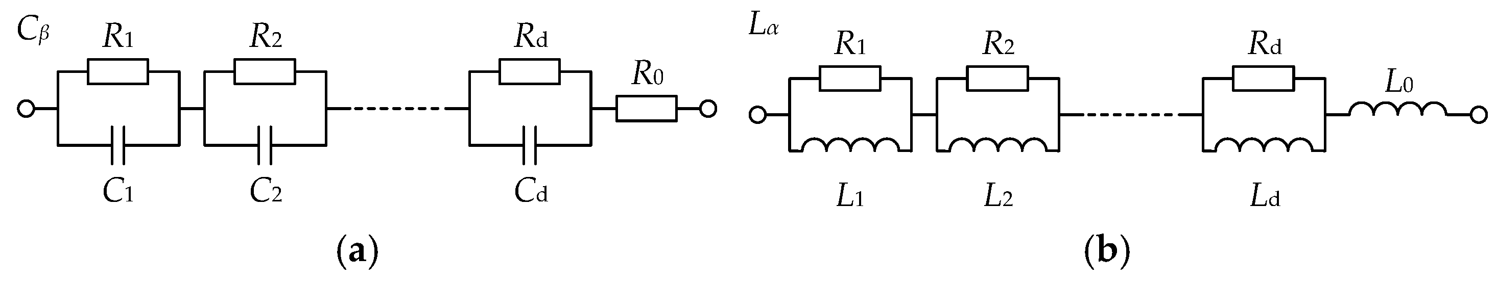
  • A simplified equivalent circuit for a fractional-order inductor is proposed, which greatly reduces the computational complexity of its parameters.
  • The existing studies on inverters are all concentrated on the fractional-order modeling and control of grid-connected inverters, this paper considered fractional-order characteristics of the resistive-inductive load in off-grid conditions.
  • Based on the double fractional-order PI controller, the transfer function between the inverter port voltage and the load voltage is derived so as to establish the complete fractional state-space mathematical model of the system in dq coordinates.
  • The impact of the fractional-order variation of the fractional-order PI controllers and the fractional elements on system performance in the frequency domain and time domain is described in detail, laying the foundation for optimizing system control.

2. HBCS-MG System Structure and Fractional Mathematical Model

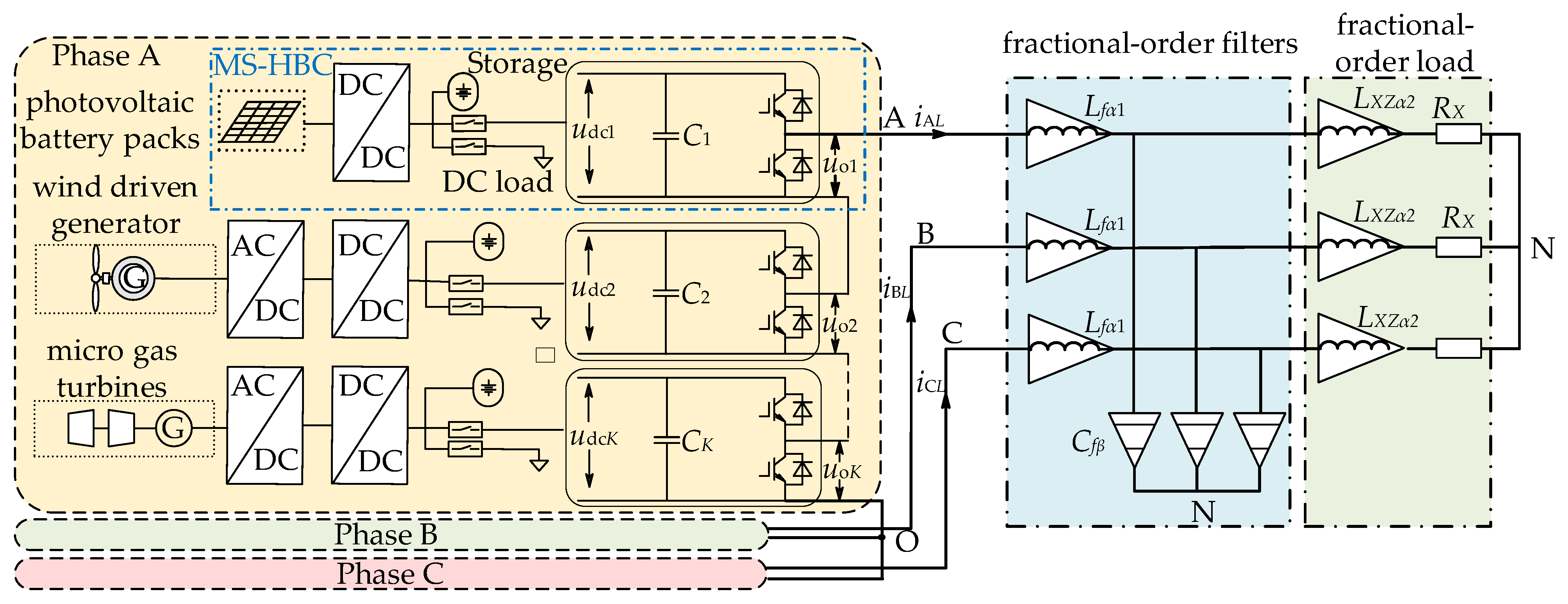
2.1. HBCS-MG System Structure

The schematic diagram of the HBCS-MG in the off-grid mode is shown in Figure 1. Each phase contains K generating units, and each generating unit is connected in series via a micro-source half-bridge converter (MS-HBC).
In Figure 1, points A, B, and C are the upper output ports of the first MS-HBC of the three phases, point O is the common connection point of the lower output port of the last MS-HBC of the three phases, and point N is the star-connection point of the load equivalent circuit. Let X = A, B, and C represent the phase sequence of three phases. Assuming the symmetry of the three-phase filter, L1 is the inductance of the filter inductor with the fractional-order of α1; C is the capacitance of the filter capacitor with the fractional-order of β; LXZα2 and RX are the inductive and resistive components in each phase load, respectively, with the fractional-order of α2. In off-grid mode, although the single-phase output voltage of the system is DC, the system is able to supply AC power to the load if it is connected in three-phase Y or ∆, due to the potential difference between points O and N. The choice of line voltage to supply the load has a higher voltage utilization, but for the purposes of simplified calculation, the circuit is equated to a three-phase Y connection.
The overall control block diagram of the system is shown in Figure 2. First, the given value of the load voltage in the dq coordinate system uCfd ** and uCfq ** is obtained through virtual synchronous generator (VSG) control. Then, a double-closed-loop FOPI control is employed, with the inner-loop for filter capacitor current control and the outer-loop for load voltage control. Finally, the modulation signals are distributed to each MS-HBC in accordance with the power demand to realize the system control.

2.2. Equivalent Circuit of the Fractional Element

The impedance of the fractional-order capacitor and inductor in the s-domain, based on Caputo’s definition, can be expressed as CZ(s) and CZ(s), respectively [28], where
Z C β C s = U C β s I C β s = 1 s β C β
Z L α C s = U L α s I L α s = s α L α
The Oustaloup algorithm can be approximated by a set of filters for the fractional-order operator sγ. Specifically, in the amplitude-frequency domain, a given frequency band is divided equally into d parts, and a first-order filter with poles and zeros in each small frequency interval is used to approximate sγ. The formula is as follows:
s γ H i = 1 d s ω i s ω i
where ω i and ω i are the zeros and poles of the integer-order filter, respectively.
A distributed expansion of Equation (3) is given as Equation (4), in which the residue, poles, and individual terms in the distributed expansion equation of sγ are represented by ri, pi, and g, respectively.
s γ = r 1 s + p 1 + r 2 s + p 2 + + r d s + p d + g
Let the fractional-order capacitor be Cβ, and its equivalent circuit is the same as that in the literature [25], as shown for Cβ in Figure 3a. The fractional-order inductor is denoted by Lα due to the complexity of the equivalent circuit of the fractional-order inductor in the existing literature. A new chain equivalent circuit of the fractional-order inductor is proposed in this paper, as shown in Figure 3b.
The impedance of the chain equivalent circuit of the fractional-order capacitor Cβ and inductor Lα is derived from Figure 3:
Z C β = 1 s β C β = i = 1 d 1 / C i s + 1 / R i C i + R 0
Z L α = L α s α = i = 1 d R i s R i / L i + s + L 0 s
For the fractional-order capacitor, the distributed expansion of sβ is first calculated, then sβ is divided by Cβ and compared with Equation (5) to obtain the size of each group of components in the chain equivalent circuit of the fractional-order capacitor, as Ci = Cβ/ri, Ri = 1/Cipi, and R0 = g/Cβ.
For the fractional-order inductor, a comparison of Equations (4) and (6) shows that the numerators differ by s. Therefore, the distributed expansion of sα−1 is first obtained and then multiplied by Lαs, which is the distributed expansion of Z. Let the residue, poles, and individual terms in the distributed expansion equation of sα−1 be ti, qi, and f, respectively. Multiplying sα−1 by Lαs and comparing with Z gives the sizes of each group of integer-order elements in the chain equivalent circuit of fractional-order inductors Ri = Lαti, Li = Ri/qi, and L0 = Lαf. This approach provides a more straightforward and computationally efficient alternative to the equivalent circuit calculation method for fractional-order inductors, as discussed in the literature [27,28].
The capacitor is selected with a capacitance of 20 μF and an order of β = 0.8. The inductor is selected with an inductance of 5 mH and an order of α = 0.9. The filter order is d = 5. The parameters of each component of the integer-order in the equivalent circuit are provided in Table 1.
Figure 4 shows the numerical impedance and equivalent circuit impedance Bode plots of the aforementioned fractional element, according to the Caputo definition. A comparison of the Bode plot of the above fractional element reveals that the amplitude-frequency characteristics of the two are essentially identical within the 10−2–104 frequency band. Consequently, the equivalent circuit of the fractional element used in this paper is considered sufficient to characterize its properties.

2.3. Fractional-Order Equivalent Circuit of the System

Let the filtered inductor current, capacitor current, load current, and load voltage in the three-phase system be iXL = [iAL iBL iCL]T, iXCf = [iACf iBCf iCCf]T, iXZ = [iAZ iBZ iCZ]T, and uXCf = [uACf uBCf uCCf]T, respectively. uXN = [uAN uBN uCN]T is the potential difference between points X and N. The single-phase equivalent circuit of the system is shown in Figure 5. The effective value of the system line voltage is 220 V when the peak value of uXCf is 180 V.
When the DC-side voltage of each MS-HBC is equal to udci, the expression for the output voltage of each phase uXO, as shown in Figure 1, is given by Equation (1) [29]. Where Mi is the modulation of the ith MS-HBC, ωc is the carrier frequency, ωs is the modulation waveform frequency, θx is the phase shift angle, m is the factor of harmonics of the carrier, and n is the factor of harmonics of the modulation waveform.
u X o = i = 1 K u X i = K u dc i 2 + i = 1 K M i u dc i 2 sin ω s t + θ x   + i = 1 K m = 1 , 3 , 5 , n = 2 u dc i m π J n m M i π 2 sin m + n 2 π ·   cos m ω c t + i 1 2 π N + n ω s t + θ x
From the principle of the three-phase star circuit, uXN can be obtained as follows in Equation (7).
u XN = u AN u BN u CN = 2 3 1 3 1 3 1 3 2 3 1 3 1 3 1 3 2 3 u Ao u Bo u Co
Neglecting the effect of harmonics, the calculation gives u X N = i = 1 N M i 2 u dc i sin ω s t + θ x .
From Figure 5, the state-space equations of the system under the three-phase stationary coordinate system are shown in Equation (9):
L f α 1 s α 1 i X L s = u X N s u X C f s C f β s β u X C f s = i X L s i X Z s L X Z α 2 s α 2 i X Z s = u X C f s u R X s
Taking phase A as an example, define G as the transfer function between uACf and uAN, then G is obtained from Equation (9):
G = R A + L A Z α 2 s α 2 L f α 1 L A Z α 2 C f β s α 1 + α 2 + β + L f α 1 s α 1 + L A Z α 2 s α 2 + R A L f α 1 C f β s α 1 + β + R A

2.4. Fractional-Order Mathematical Model of the System in Rotating Coordinates

When the system is in the three-phase symmetrical case, the abc/dq transform matrix of the sine function is shown in Equation (11).
P = 2 3 sin ω s t sin ω s t 2 3 π sin ω s t + 2 3 π cos ω s t cos ω s t 2 3 π cos ω s t + 2 3 π
The formula for the fractional derivative of a trigonometric function, according to Caputo’s definition, is as Equation (12), where D t γ f ( t ) is the γth derivative [24]:
D t γ sin ω s t = a γ sin ω s t + γ π / 2
D t γ cos ω s t = a γ cos ω s t + γ π / 2
Equations (12) and (13) are used to derive the fractional-order derivative of the trigonometric function in the inverse matrix of (11), which is then multiplied by P, yielding (14):
P d γ P d t γ = ω s cos α γ π 2 ω s sin α γ π 2 ω s sin α γ π 2 ω s cos α γ π 2
If α = 1, then P d α P d t α = 0 ω ω α   0 is consistent with integer-order.
Let iLd/q, uXNd/q, uCfd/q, iZd/q, uZd/q, and iCfd/q be the representations of iXL, iXN, uXCf, iXZ, uRX, and iXCf in dq coordinates, respectively. Combined with Equations (9) and (14), the state-space model of the HBCS-MG off-grid system in dq coordinates is shown in (15).
i L d / q s G l 1 = u X Nd / q s u C f d / q s ± L f α 1 ω α 1 sin α 1 π 2 i L q / d s u C f d / q s G c = i L d / q s i Z d / q s ± C f β ω β sin β π 2 u C f q / d s i Z d / q s G l 2 = u C f d / q s u R d / q s ± L Z α 2 ω α 2 sin α 2 π 2 i Zq / d s
Gl1, Gc, and Gl2 are as follows:
G l 1 = 1 / L f α 1 s α 1 + L f α 1 ω α 1 cos α 1 π 2
G c = 1 / C f β s β + C f β ω β cos β π 2
G l 2 = 1 / L Z α 2 s α 2 + L Z α 2 ω α 2 cos α 2 π 2

3. Fractional-Order Double-Closed-Loop Control of the System

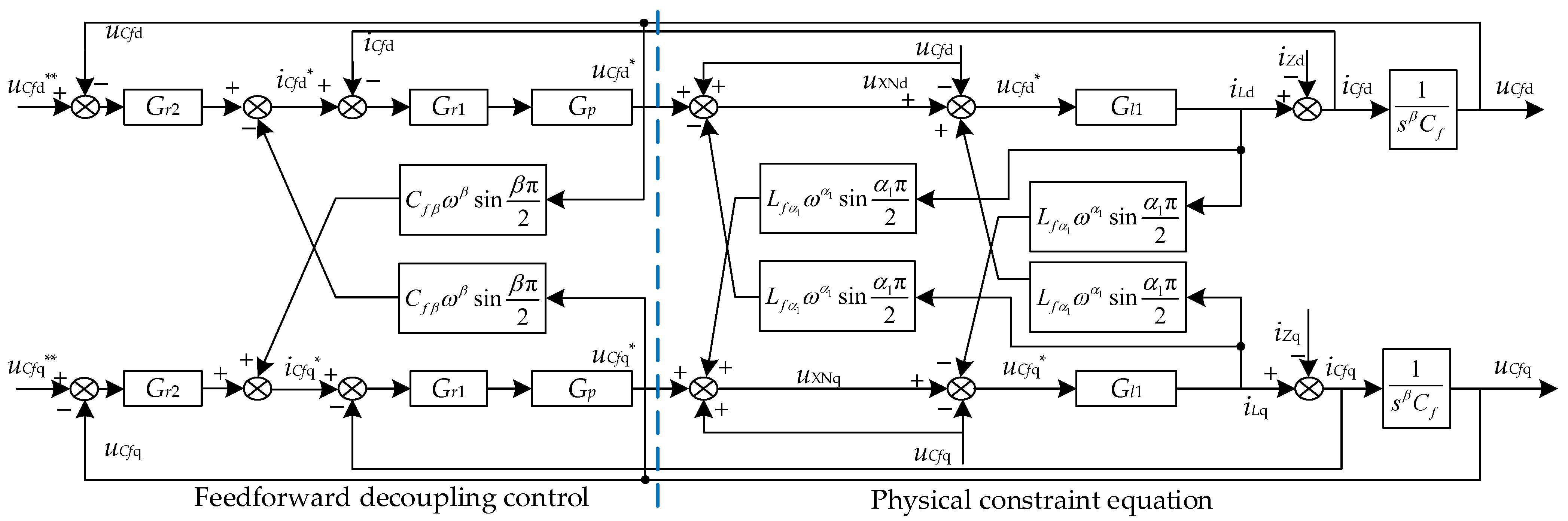
3.1. Fractional-Order Decoupling Control

As can be observed from the analysis of Equation (15), the system exhibits a nonlinear coupling phenomenon. In this paper, the load voltage feedforward control is employed to compensate for the effect of voltage fluctuations on the control of the system. The system control block diagram is shown in Figure 6, where Grk (k = 1, 2 representing the inner- and outer-loops of the control system, respectively) is the transfer function of the FOPI controller, αrk is the order of the integral term in the transfer function of the fractional-order PI controller, Gp is the SPWM gain, and uCfd ** and uCfq ** are the given values of the dq-axis output load voltage, obtained by VSG control.
The transfer function of the FOPI controller is Grk, as shown in (19).
G r k = K p k + K i k s α r k
The reference value of the dq-axis load voltage is as follows:
u C f d * = i C f d * i C f d G r 1 G p
u C f q * = i C f q * i C f q G r 1 G p
According to the left side of Equation (15), two new variables, Md and Mq, are introduced:
M d = i L d s / G l 1
M q = i L q s / G l 1
The current inner-loop decoupling control is achieved when the equations u C f d * = M d and u C f q * = M q are satisfied. Similarly, the voltage outer-loop dq-axis decoupling is realized when Equation (24) is satisfied.
i C f d / q * = 1 G c u C f d / q s = u C f d / q * * u C f d / q G r 2
Using the d-axis as an example, the control block diagram of the double-closed-loop control system after decoupling is shown in Figure 7.

3.2. Transfer Function of the Fractional-Order Double-Closed-Loop Control System

The transfer function of the system’s inner-loop current in dq coordinates is obtained from Figure 7:
G i b = i C f d i C f d * = G r 1 G p G l 1 s β C f β + G l 1 + 1 / R + s α 2 L Z α 2 + G r 1 G p G l 1 C f β s β
The transfer function of the system with the inner-loop closed and the outer-loop open is given by Equation (26).
G k 1 = u C f d u C f d ** = G r 1 G r 2 G p G l 1 R + s α 2 L Z α 2 s β C f β R + s α 2 L Z α 2 + 1 + G l 1 R + s α 2 L Z α 2 + G r 1 G p G l 1 s β C f β R + s α 2 L Z α 2   = G p b 1 s n b 1 + b 2 s n b 2 + + b 7 s n b 7 + b 8 a 1 s n a 1 + a 2 s n a 2 + + a 8 s n a 8 + a 9
The transfer function of the voltage and current double-closed-loop control system is given by Equation (27).
G u b = G r 2 G r 1 G p G l 1 s β C f β 1 + G r 1 G p G l 1 + 1 R + s α 2 L Z α 2 + G l 1 + G r 2 G r 1 G p G l 1   = G p b 1 s n b 1 + b 2 s n b 2 + + b 7 s n b 7 + b 8 a 1 s n a 1 + a 2 s n a 2 + + a 8 s n a 8 + G p c 1 s n c 1 + c 2 s n c 2 + + c 7 s n c 7 + c 8
Note: ai, nai, bi, nbi, ci, and nci are listed in the Appendix A.
Equation (27) and Appendix A show that the full fractional-order mathematical model constructed has 15 orders, and 12 control parameters need to be adjusted, taking into account the impedance values of the three fractional reactance elements and the fractional-order, which is of some complexity. Therefore, it is of practical significance to accurately model and analyze the operating characteristics of the off-grid microgrid under different parameters, which can lay a foundation for the subsequent optimization of the controller parameters.

4. Effect of the Fractional-Order Controller on System Performance

To verify the accuracy of the fractional-order mathematical model of the HBCS-MG system in the off-grid state and analyze the effects of variations in αrk on performance, this section presents both the characterization of the system transfer function and the electrical characteristics obtained from the simulation.
The power component of the simulation model is shown in Figure 1. The equivalent circuit of the fractional element based on the Oustaloup filter is used to construct the filter inductor and the inductive component of the load. The simulation time is 1 s, and the load change is divided into three steps, with the impedance angle of Z3 being larger than Z2. The simulation parameters are shown in Table 2 and Table 3.

4.1. Amplitude-Frequency Characteristics of αrk Variation with the Outer-Loop Opened

The filter parameters are presented in Table 1. Under load Z2, from Equation (26), the frequency domain characteristics of the system with αr1 and αr2 varied within the frequency range of 10−1–107 rad/s are shown in Table 4 and Table 5. When αr1 = αr2, the variation in the Bode plots of the transfer function Gk1 is shown in Figure 8.
By examining Figure 8 and Table 4 and Table 5 together, it is evident that in this case, when both αr1 and αr2 are small (<0.5) or large (>1.5), the amplitude margin or phase margin of Gk1 becomes negative. Therefore, the system’s stability must be evaluated in conjunction with its dynamic response characteristics. When either αr1 or αr2 falls between 0.5 and 1.5, no crossover frequency exists within the 10−1–107 rad/s range, indicating that the system remains stable.

4.2. Characterization of the System Step Response as αrk Varies

The step response waveform of Gub is plotted to obtain its peak value, peak value time, and steady-state time when αrk varies, and the data are presented in Table 6, Table 7 and Table 8, respectively. In the table, arrow ↑ indicates an upward trend, ↓ indicates an downward trend. NaN indicates inexistence.
As illustrated in Table 6, when either αr1 or αr2 is relatively small (αrk < 0.7), and only one of them is increased, the peak value first increases, then decreases and increases again. However, the second increase is significantly smaller than the first. If either αr1 or αr2 is increased to some extent (αrk ≥ 0.7), an increase in only one of them (change term < 1.5) will cause the peak to first increase and then decrease. If either αr1 or αr2 is further increased (αr1 > 1 or αr2 > 1.3), the peak will continue to increase with the change term until a point of instability is reached. Additionally, the impact of a simultaneous increase in αrk on the peak value of the step response is more pronounced than that of an increase in a single term. From Table 7, it can be seen that the peak value time increases as αr1 or αr2 increases.
As illustrated in Table 8, the steady-state time increases as αrk increases. When both αr1 and αr2 ≥ 1.4, the step response curve oscillates, and the system is in an unstable state, there is no peak value. In general, the impact of a change in either αr1 or αr2 on the peak value of the step response and steady-state time of the system is symmetrically distributed.
Taking αr1 = αr2 = 0.8 as an example under the step response, the overshooting amount is 11.6%, a reduction of 7.3% compared with the integer-order case, the peak time is 0.0051 s, a decrease of 0.013 s compared with the integer-order case, and the steady-state time is shortened by 0.065 s. It is shown that the fractional-order PI control outperforms the integer-order PI control.

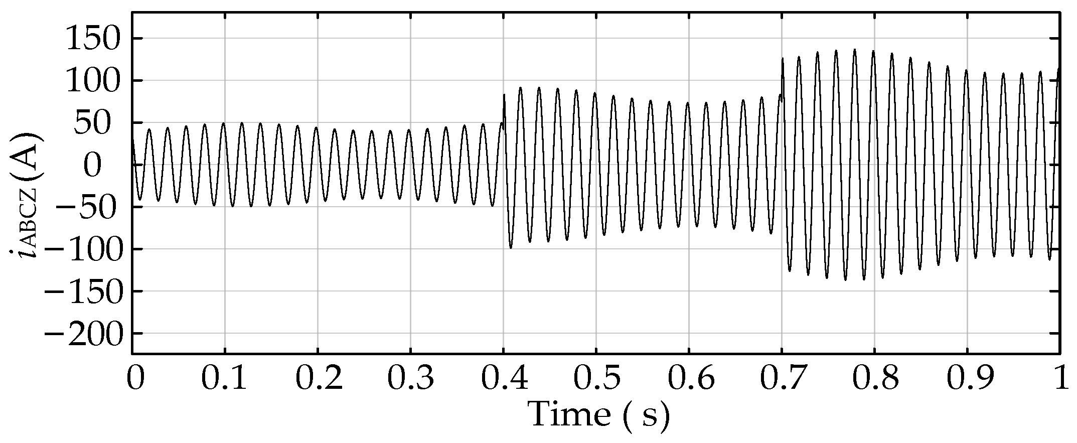
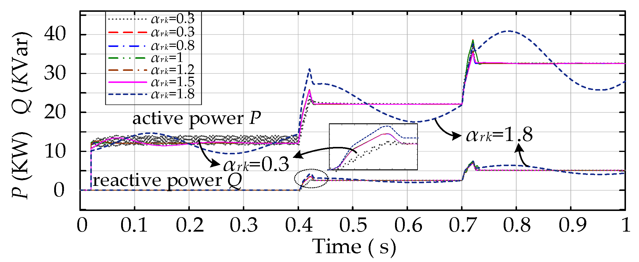
4.3. Electrical Characterization of the System as αrk Changes

The filter parameters are kept constant, and the simulation is carried out with αr2 = 0.8 and αr1 varied as an example. The variation of the system’s output voltage is shown in Table 9. Table 10 illustrates the impact of synchronous variation in αrk on the load voltage. Where up denotes the peak value of the voltage at the instant of load switching, uw denotes the amplitude of the steady-state voltage after load switching.
Table 9 illustrates that at 0.4 s, there is an increasing and then decreasing trend with increasing αr1, which coincides with the peak of the step response. In the simulation, it should be noted that the maximum of up is observed at αr1 = 0.6, while the peak of the step response is observed at αr1 = 0.8. This is due to the inclusion of VSG control in the simulation, which permits a broader range of fractional-order adjustment for the controller. Moreover, modifying only αr1 has a negligible impact on uw and its total harmonic distortion (THD). Similarly, the simulation indicates that modifying only αr2 has the same impact on uw and its THD as modifying only αr1. Therefore, this result is not presented again.
As can be seen from Table 10, different from the theoretical calculations where the peak value of the step response increases continuously with the increase of αrk, the up at 0.4 s does not differ significantly at αrk ∈ [0.5, 1.5], and it reaches its maximum at αrk = 1.8. This is also due to the addition of the VSG control, which improves the stability of the system. The integer-order PI controller is not in an optimal state with regard to its voltage response under load disturbance. At 0.7 s, the peak value under integer-order PI control is 196.4 V, while when αr1 = αr2 = 0.8, the peak value of the load voltage is 187.9 V, a reduction of 4.2%. This indicates that the FOPI controller improves the control accuracy of the system.
When αrk = 0.3, the THD of uw under Z1 load is 126%, which indicates an unstable state. In contrast, the system shows relatively stable behavior under Z2 and Z3 loads. When αrk = 1.8, the stability of the system is significantly impaired, exceeding the regulatory limits of the VSG control and resulting in an unstable state. Additionally, the THD of Z3 is higher than Z1 and Z2. Therefore, a moderate increase in αrk when the impedance angle declines and a moderate decrease in αrk when the impedance angle rises in the load will assist in reducing THD in the load voltage.
The waveform of the system load current as αrk varies is shown in Figure 9, Figure 10 and Figure 11. From these figures, it can be seen that the current oscillation is mainly observed under a resistive load when αrk = 0.3 and that the load current amplitude exhibits a sustained oscillation when αrk = 1.8.
Figure 12 shows the variation of load power with αrk. It can be seen that when αrk is small, the active power variation under a resistive load is greater than that under a resistive-inductive load. As αrk increases, the impact on the active power of the load also increases.
In conclusion, αrk being either too low or too high will result in a deterioration of the system performance. If αrk is set too low, it will mainly affect the voltage quality of resistive loads. It should be noted that αrk has a relatively small effect on reactive power. Comparison of the system transfer function characteristics with the electrical characteristics proves the accuracy of the proposed model.

5. Effect of the Fractional-Order of the Fractance Element on System Performance

This section also analyzes the effect of variations α1, β, and α2 on the system performance, both in terms of the system transfer function characteristics and the electrical characteristics obtained from the simulation.

5.1. Effect of Changing α1 on System Performance

5.1.1. Amplitude-Frequency Characteristics of α1 Variation with the Outer-Loop Opened

When αr1 = αr2 = 0.8, β = 0.8, and α2 = 0.9, the Bode plot of the system’s outer-loop open transfer function Gk1 as α1 is varied is shown in Figure 13. Let the amplitude margin be defined as h, the phase-angle margin as γ, the crossover frequency as ωx, and the cut-off frequency as ωc. The typical data of the Bode plot characteristics are presented in Table 11.
Combined with Figure 13 and Table 11, it can be seen that when α2 and β are held constant and α1 ≤ 1, with the increase of α1, the amplitude remains relatively constant in the low-frequency band but gradually decreases in the high-frequency band. This is accompanied by a reduction in the cut-off frequency and phase-angle margin, as well as a phase decreasing and approaching −180°. When α1 = 1.2, the phase-frequency curve is tangent to −180° in the high-frequency range, and although the stability margin decreases, the system remains stable.
When α1 reaches a certain threshold (α1 > 1.2), α1 variations affect the amplitude-frequency curves in all frequency bands, and the phase-angle margin shifts from positive to negative. A phase traversal of −180° occurs in both the high and low-frequency bands, and the amplitude margin is reduced, resulting in an unstable system state.

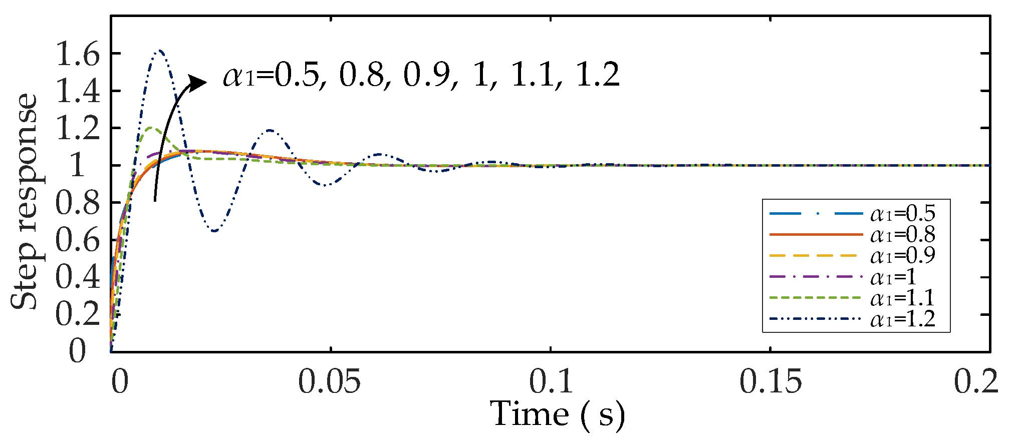
5.1.2. Effect of Changing α1 on the Dynamic Response Characteristics of the System

The step response waveform of the double-closed-loop system as α1 changes is shown in Figure 14. From the step response waveform of the system as α1 changes, it can be observed that an increase in α1 results in a higher peak of the step response and a longer steady-state time.

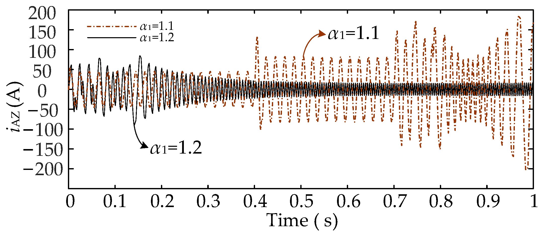
5.1.3. Electrical Characterization of the System as α1 Change

As α1 is varied, the simulation demonstrates the variation of uw, as shown in Table 12. It can be seen that as α1 increases, the THD of the load voltage decreases while the uw remains constant. When α1 is increased to 1.2, the load voltage becomes unstable. The THD of uw is at a minimum when α1 = 1.1, indicating that the introduction of a fractional-order filter improves the stability of the system.
Figure 15 illustrates the 0.4 s local amplification waveform of the load current. It can be observed that an increase in α1 results in a corresponding rise in the transient peak value of the load current, which is consistent with the peak value characteristic of the transfer function step response.
When α1 = 1.1 and 1.2, the load current waveform of phase A is shown in Figure 16. It can be seen that when α1 = 1.1, the grid requirements can be met under both the resistive load Z1 and the resistive-inductive load Z2. However, as the load and its power factor increase, the system becomes unstable. As α1 is further increased (α1 = 1.2), the load voltage cannot meet the grid requirements under either load. This indicates that reducing the load impedance angle will increase the adjustable range of α1.
The load power waveform as α1 changes is shown in Figure 17. From its local amplification curve, it can be observed that as α1 increases (α1 ∈ {0.6, 0.8, 1}), the peak of the load active power at 0.4 s increases and the response speed slows down. This indicates that the stability margin decreases, which is consistent with the theoretical analysis and proves the accuracy of the constructed mathematical model. As the load power factor increases, the impact of α1 on the power output becomes more evident. Once α1 ≥ 1.1, the active power output of the system is unable to align with the load demand.
In conclusion, if α1 is either too high or too low, this will affect the power quality of the system. Reducing α1 to an insufficient level will affect the filtering effectiveness of the system output voltage, while increasing α1 to an excessive level will primarily affect the stability of the system output voltage. The effect of α1 on resistive-inductive loads is more significant than on resistive loads, and the larger the impedance angle, the easier it is to cause system instability.

5.2. Effect of Changing β on System Performance

5.2.1. Amplitude-Frequency Characteristics of β Variation with the Outer-Loop Opened

When α1 and α2 are set to 0.9, all other circuit and control parameters remain unaltered. The Bode plot of the outer-loop open transfer function of the system as β is varied is shown in Figure 18. Typical data for the corresponding characteristic curves are presented in Table 13.
Combined with Figure 18 and Table 13, when α1 and α2 are held constant, an increase in β has a negligible impact on the low-frequency band, which only affects the high-frequency band, and the cut-off frequency remains largely unaltered when β is less than 1.2. Given the minimal impact of the high-frequency band on the actual amplitude, β has a negligible influence on the stability margin of the system within the stabilization interval. Once β ≥ 1.4, the phase-angle margin becomes negative, and the stability of the system must be determined in conjunction with other characteristics.

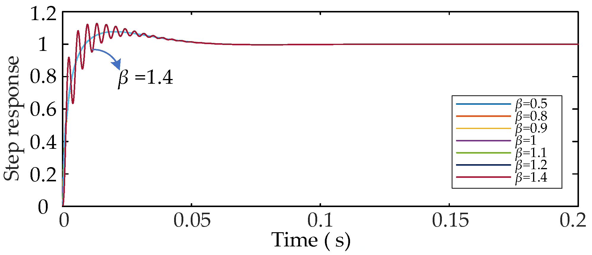
5.2.2. Effect of Changing β on the Dynamic Response Characteristics of the System

The step response waveforms of the double-closed loop control system as β changes are illustrated in Figure 19. From the figure, it can be observed that the load step response characteristics are almost identical when the fractional-order of the capacitor is less than 1.4. When β is equal to 1.4, the oscillation frequency of the step response curve increases while the steady-state time remains unaltered. Consequently, the impact of modifying the fractional-order of the capacitor on the system’s output is found to be insignificant.

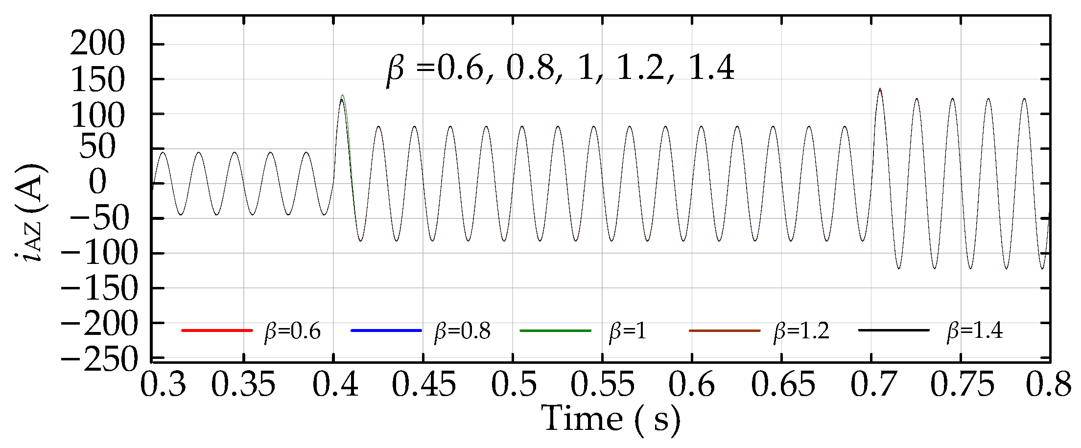
5.2.3. Electrical Characterization of the System as β Vary

As β is varied, the simulation shows the variation in the steady-state value of the system output voltage, as shown in Table 14. An examination of the data presented in Table 14 reveals that the value of β does not influence the steady-state value of the system load voltage. However, when β is set to a value of 0.6 or below, it has an impact on the quality of the load voltage waveform, although the amplitude remains stable. An increase in β facilitates an improvement in the quality of the load voltage.
The load current waveforms as β is varied are presented in Figure 20. As can be observed from the figure, the load current waveforms exhibit a high degree of overlap as β is varied. In conclusion, the alteration of the fractional-order of the filter capacitor has a negligible influence on the load steady-state current, and the simulation results are consistent with the theoretical analysis.

5.3. Effect of Changing α2 on System Performance

5.3.1. Amplitude-Frequency Characteristics of α2 Variation with the Outer Loop Opened

When β = 0.8, α1 = 0.9, and α2 is varied, the Bode plot of the transfer function Gk1 is shown in Figure 21. The characteristic data are given in Table 15.
Combined with Figure 21 and Table 15, it can be seen that when α2 ≤ 1, overall, the amplitude increases with α2 in the low-frequency band. However, in the high-frequency band, the amplitude and phase essentially overlap, resulting in a negligible increase in the cut-off frequency and a minimal reduction in phase-angle margin. As α2 increases, the stability margin is abruptly reduced after α2 > 1, resulting in a decline in stability.

5.3.2. Effect of Changing α2 on the Dynamic Response Characteristics of the System

Figure 22 shows the step response waveforms of the double-closed-loop system when changing α2. From the local amplification waveform at the peak value in Figure 22, it can be observed that as α2 continues to increase, the peak value of the system step response also gradually increases. Nevertheless, the extent of this alteration is considerably less than that of the influence exerted by α1 on the peak value of the step response.

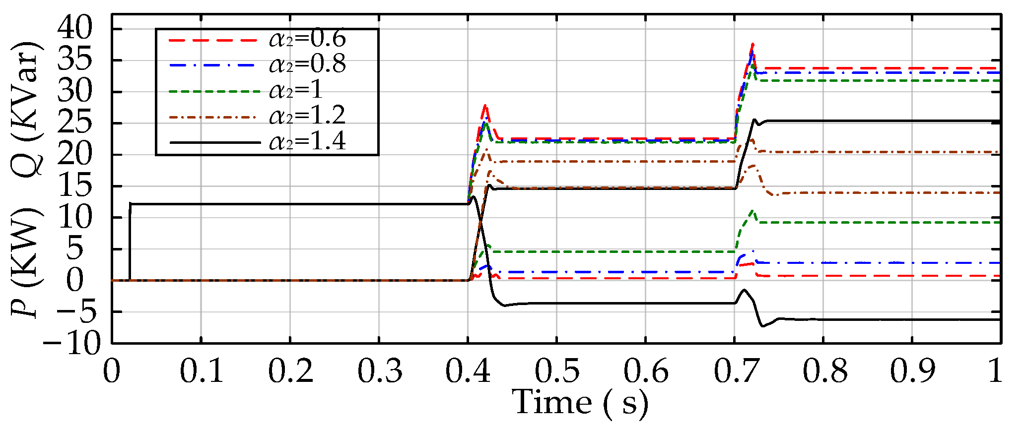
5.3.3. Electrical Characterization of the System as α2 Varies

Table 16 shows the variation in the steady-state value of the load voltage as α2 changes. It can be seen that with α2 = 0.8 as the reference, an increase or decrease in α2 results in a reduction in the quality of the system output voltage. Furthermore, when α2 is set to 1.4, the voltage of the resistive-inductive load becomes unstable.
Figure 23 illustrates the locally amplified waveform of the load current as α2 varies. It can be observed that an increase in α2 is equivalent to an increase in the load impedance in the microgrid, which consequently leads to a reduction in the load current.
The load power waveforms as α2 varies are presented in Figure 24. It can be observed that as α2 increases, there is a corresponding decrease in the active power demand of the microgrid, accompanied by an increase in the reactive power demand. When α2 reaches a certain level, the load will release active power in reverse, while reactive power will continue to increase.
In conclusion, the alteration in α2 affects the equivalent impedance of the inductive component within the load. An increase in α2 results in a higher impedance and a larger power factor angle. Consequently, the load current, active power, and reactive power are all affected. Compare the effects of changes in α1, β, and α2 on the frequency domain characteristics and electrical characteristics of the system to demonstrate the correctness of the model developed.

6. Conclusions

This paper employs the HBCS-MG system as a background, considers the fractional-order characteristics of the filter inductor, filter capacitor and load inductive components, and adopts a double-closed-loop control strategy with FOPI controllers for the purpose of analyzing the effects of fractional-order changes in the controller and each fractional element on the output characteristics of the system.
The optimal fractional-order range of FOPI controllers and fractional elements is shown in Table 17.
The results demonstrate that the introduction of a FOPI controller into a double-closed-loop control system improves the accuracy of the control system. When αrk is set to a low value, it mainly affects the voltage quality of the resistive load. The impact of the fractional-order changes of the three fractional elements, namely the filter inductor, the inductive load component and the filter capacitor, on the output voltage of the system diminishes in a sequential manner. If the controller parameters remain unchanged and the fractional-order of the filter inductance and filter capacitor is insufficient, the filtering effect will be reduced, although stability is maintained. If the fractional-order of the filter inductance and load inductance is excessive, the system will become unstable. Furthermore, the filter capacitance has a negligible impact on the output characteristics of the system. The adjustable range of the filter inductance fractional-order is less extensive under a resistive load than under an inductive load. An increase in the fractional-order of the load inductance will result in a reduction in active power and an increase in reactive power at the load. The comparison between the frequency domain characteristics and the electrical characteristics demonstrates the correctness of the complete fractional mathematical model.

7. Discussion

The use of fractional-order control helps to improve the accuracy of microgrid control. Although this study has provided a detailed analysis of the impact of changing the fractional-order of the controller and the fractional elements within the system on the output characteristics, the following challenges exist in its implementation.
(1) Fractional-order controllers involve non-integer-order calculus operations, which may lead to real-time problems in embedded systems or real-time control systems with limited computational resources.
(2) Traditional analog or digital controllers are usually based on integer-order differentiation, and direct implementation of fractional-order controllers requires special numerical computation methods.
(3) Because the fractional-order characteristics of components are usually related to environmental factors such as frequency and temperature, it is a challenge to accurately model and optimize the controller parameters under different operating conditions.

Author Contributions

Formal analysis, Y.D.; Data curation, H.W. and Y. D; Writing—original draft, Y.D.; Writing—review & editing, Y.D., X.W., L.Z., H.W. and J.L. All authors have read and agreed to the published version of the manuscript.

Funding

This research was supported by the National Natural Science Foundation of China, 51967011.

Institutional Review Board Statement

Not applicable.

Data Availability Statement

Data are contained within the article.

Conflicts of Interest

The authors declare no conflicts of interest.

Abbreviations

HBCS-MGHalf-bridge converter series microgrid
FOPIFractional-order PI
SMSI-MGMicrogrid with series micro-source inverters
MMC-MGModular multilevel converter half-bridge series microgrid
WECSWind energy conversion system
HESGHybrid excitation synchronous generator
FOVSRFractional-order voltage source PWM rectifier
MS-HBCMicro-source half-bridge converter
VSGVirtual synchronous generator
THDTotal harmonic distortion

Appendix A

b 1 = K p 1 K i 2 R b 2 = K p 2 K i 1 R b 3 = K i 1 K i 2 R b 4 = K p 1 K i 2 L Z α 2 b 5 = K p 2 K i 1 L Z α 2 b 6 = K i 1 K i 2 L Z α 2 b 7 = K p 1 K p 2 L Z α 2 b 8 = K p 1 K p 2 R n b 1 = α r 2 n b 2 = α r 1 n b 3 = α r 1 α r 2 n b 4 = α r 2 + α 2 n b 5 = α r 1 + α 2 n b 6 = α r 1 α r 2 + α 2 n b 7 = α 2
a 1 = L f α 1 C f β R a 2 = L Z α 2 a 3 = L f α 1 a 4 = L f α 1 C f β L Z α 2 a 5 = K i 1 G p C f β R a 6 = K i 1 G p C f β L Z α 2 a 7 = C f β L f α 1 R ω α 1 cos α 1 π 2 + K p 1 G p C f β R a 8 = C f β L f α 1 L Z α 2 ω α 1 cos α 1 π 2 + K p 1 G p C f β L Z α 2 a 9 = L f α 1 ω α 1 cos α 1 π 2 n a 1 = β + α 1 n a 2 = α 2 n a 3 = α 1 n a 4 = β + α 1 + α 2 n a 5 = β a r 1 n a 6 = a 2 + β α r 1 n a 7 = β n a 8 = β + α 2
c 1 = K p 1 K i 2 R c 2 = K p 2 K i 1 R c 3 = K i 1 K i 2 R c 4 = K p 1 K i 2 L Z α 2 c 5 = K p 2 K i 1 L Z α 2 c 6 = K i 1 K i 2 L Z α 2 c 7 = K p 1 K p 2 L Z α 2 c 8 = L f α 1 ω α 1 cos α 1 π 2 + R + G p K p 1 K p 2 R n c 1 = α r 2 n c 2 = α r 1 n c 3 = α r 1 α r 2 n c 4 = α r 2 + α 2 n c 5 = α r 1 + α 2 n c 6 = α r 1 α r 2 + α 2 n c 7 = α 2

References

  1. Hou, N.; Ding, L.; Gunawardena, P.; Wang, T.H.; Zhang, Y.; Li, Y.W. A Partial Power Processing Structure Embedding Renewable Energy Source and Energy Storage Element for Islanded DC Microgrid. IEEE Trans. Power Electron. 2020, 36, 2499–2504. [Google Scholar] [CrossRef]
  2. Zheng, H.Y.; Song, M.L.; Shen, Z.Y. The evolution of renewable energy and its impact on carbon reduction in China. Energy 2021, 237, 121639. [Google Scholar] [CrossRef]
  3. Severino, B.; Strunz, K. Enhancing transient stability of DC microgrid by enlarging the region of attraction through nonlinear polynomial droop control. IEEE Trans. Circuits Syst. I Reg. Pap. 2019, 66, 4388–4401. [Google Scholar] [CrossRef]
  4. Li, D.S.; Sun, Q.Y.; Wang, R.; Sui, Z. Transient Stability Analysis and Enhancement of Inverter-Based Microgrid Considering Current Limitation. IEEE Trans. Power Electron. 2025, 40, 2429–2441. [Google Scholar] [CrossRef]
  5. Hu, J.F.; Shan, Y.H.; Yang, Y.; Parisio, A.; Li, Y.; Amjady, N. Economic Model Predictive Control for Microgrid Optimization: A Review. IEEE Trans. Smart Grid 2024, 15, 472–484. [Google Scholar] [CrossRef]
  6. Wang, X.G.; Ding, Y.J.; Li, J.J.; Guo, Y.J. Characteristics analysis of micro-source half-bridge converter series Y-connection based microgrid systems. J. Power Electron. 2023, 23, 1483–1495. [Google Scholar] [CrossRef]
  7. Wang, X.G.; Li, J.J.; Guo, Q.; Wang, H.L.; Ding, Y.J. Parameter design of half-bridge converter series Y-connection microgrid grid-connected filter based on improved PSO-LSSVM. Int. Trans. Electr. Energy Syst. 2023, 2023, 9534004. [Google Scholar] [CrossRef]
  8. Yu, D.H.; Liao, X.Z.; Wang, Y. Modeling and analysis of Caputo–Fabrizio definition-based fractional-order boost converter with inductive loads. Fractal Fract. 2024, 8, 81. [Google Scholar] [CrossRef]
  9. Govind, D.; Suryawanshi, H.M.; Nachankar, P.P.; Narayana, C.L.; Singhal, A. Fractional-order LC filter modeling, implementation, and analysis for distributed power generation system. Int. J. Circuit Theory Appl. 2023, 51, 4565–4583. [Google Scholar] [CrossRef]
  10. El-Khazali, R. Fractional-order LCαL filter-based grid connected PV systems. In Proceedings of the 2019 IEEE 62nd International Midwest Symposium on Circuits and Systems (MWSCAS), Dallas, TX, USA, 4–7 August 2019; pp. 533–536. [Google Scholar]
  11. Kashfi, R.; Balochian, S.; Alishahi, M. Design of a optimal robust adaptive neural network-based fractional-order PID controller for H-bridge single-phase inverter. Appl. Soft Comput. 2024, 166, 112142. [Google Scholar] [CrossRef]
  12. Zhao, C.N.; Jiang, M.R.; Huang, Y.Q. Formal verification of fractional-order PID control systems using higher-order logic. Fractal Fract. 2022, 6, 485. [Google Scholar] [CrossRef]
  13. Tumari, M.Z.M.; Ahmad, M.A.; Rashid, M.I.M. A fractional order PID tuning tool for automatic voltage regulator using marine predators algorithm. Energy Rep. 2023, 9, 416–421. [Google Scholar] [CrossRef]
  14. Krishna, P.S.; Rao, P.V.G.K. Fractional-order PID controller for blood pressure regulation using genetic algorithm. Biomed. Signal Process. Control 2024, 88, 105564. [Google Scholar] [CrossRef]
  15. Gokyildirim, A.; Calgan, H.; Demirtas, M. Fractional-Order sliding mode control of a 4D memristive chaotic system. J. Vib. Control 2023, 30, 7–8. [Google Scholar] [CrossRef]
  16. Mseddi, A.; Dhouib, B.; Zdiri, M.A.; Alaas, Z.; Naifar, O.; Guesmi, T.; Alshammari, B.M.; Alqunun, K. Exploring the Potential of Hybrid Excitation Synchronous Generators in Wind Energy: A Comprehensive Analysis and Overview. Process 2024, 12, 1186. [Google Scholar] [CrossRef]
  17. Mseddi, A.; Wali, K.; Abid, A.; Naifar, O.; Rhaima, M.; Mchiri, L. Advanced modeling and control of wind conversion systems based on hybrid generators using fractional order controllers. Asian J. Control 2024, 26, 1103–1119. [Google Scholar] [CrossRef]
  18. Mohamed, A.T.; Mahmoud, F.M.; Swief, R.A.; Said, L.A.; Radwan, A.G. Optimal fractional-order PI with DC-DC converter and PV system. Ain Shams Eng. J. 2021, 12, 1895–1906. [Google Scholar] [CrossRef]
  19. Fang, S.C.; Wang, X.G. Modeling and analysis method of fractional-order buck-boost converter. Int. J. Circuit Theory Appl. 2020, 48, 1493–1510. [Google Scholar] [CrossRef]
  20. Chen, Y.F.; Wang, X.; Zhang, B.; Xie, F.; Chen, S. Differences between Riemann-Liouville and Caputo calculus definitions in analyzing fractional boost converter with discontinuous-conduction-mode operation. Int. J. Circuit Theory Appl. 2024, 52, 4164–4183. [Google Scholar] [CrossRef]
  21. Yang, N.N.; Wu, C.J.; Jia, R.; Liu, C.X. Modeling and characteristics analysis for a buck-boost converter in pseudo-continuous conduction mode based on fractional calculus. Math. Probl. Eng. 2016, 2016, 6835910. [Google Scholar] [CrossRef]
  22. Xu, J.H.; Li, X.C.; Meng, X.R.; Qin, J.B.; Liu, H. Modeling and analysis of a single-phase fractional-order voltage source pulse width modulation rectifier. J. Power Sources 2020, 497, 228821. [Google Scholar] [CrossRef]
  23. Xu, J.H.; Li, X.C.; Liu, H.; Meng, X.R. Fractional-order modeling and analysis of a three-phase voltage source PWM rectifier. IEEE Access 2020, 8, 13507–13515. [Google Scholar] [CrossRef]
  24. Lei, Y.; Xiong, H.J.; Lei, D.M. Fractional order PID control strategy for modular multilevel converters. In Proceedings of the 2017 International Conference on Industrial Informatics—Computing Technology, Intelligent Technology, Industrial Information Integration (ICIICII), Wuhan, China, 2–3 December 2017; pp. 223–226. [Google Scholar]
  25. Wang, X.G.; Cai, J.H. Grid-Connected inverter based on a resonance-free fractional-order LCL filter. Fractal Fract. 2022, 6, 374. [Google Scholar] [CrossRef]
  26. Li, X.C.; Luo, X.L.; Hou, L.L.; Xu, J.H. Research on grid-side control of wind power generation based on fractional LCL filter. Acta Energ. Sol. Sin. 2022, 43, 383–391. [Google Scholar] [CrossRef]
  27. Li, X.C.; Hou, L.L.; Luo, X.L.; Xu, J.H. Research on fractional modeling and controller design of three-phase inverter grid-connected system. Acta Energ. Sol. Sin. 2023, 44, 415–424. [Google Scholar] [CrossRef]
  28. Liao, X.Z. Fractional Modelling and Analysis of Fractional Order RLC Circuit Systems; China Science Publishing & Media Ltd. (CSPM): Beijing, China, 2023; pp. 18–27. [Google Scholar]
  29. Li, B.B.; Yang, R.F.; Xu, D.D.; Wang, G.L.; Wang, W.; Xu, D.G. Analysis of the phase-shifted carrier modulation for modular Multilevel converters. IEEE Trans. Power Electron. 2015, 30, 297–310. [Google Scholar] [CrossRef]
Figure 1. Schematic diagram of HBCS-MG in the off-grid state.
Fractalfract 09 00202 g001
Figure 2. System’s overall control block diagram.
Fractalfract 09 00202 g002
Figure 3. Equal circuit of fractional element. (a) Fractional-order capacitance equivalent circuit; (b) fractional-order inductor equivalent circuit.
Fractalfract 09 00202 g003
Figure 4. The Bode diagram of the Caputo-type fractional capacitance and inductance impedance. (a) The Bode diagram of the Caputo-type fractional capacitance; (b) the Bode diagram of the Caputo-type fractional inductance impedance.
Fractalfract 09 00202 g004
Figure 5. Single-phase equivalent circuit of the system.
Fractalfract 09 00202 g005
Figure 6. Fractional-order PI control block diagram of the system. The blue line is used to distinguish between decoupled control and physical constraint equations.
Fractalfract 09 00202 g006
Figure 7. The system double-closed-loop control structure diagram after decoupling.
Fractalfract 09 00202 g007
Figure 8. The Bode diagram when αrk changes synchronously.
Fractalfract 09 00202 g008
Figure 9. System phase A load current at αrk = 0.3.
Fractalfract 09 00202 g009
Figure 10. System load current at αrk = 0.5, 0.8, 1, 1.2, 1.5.
Fractalfract 09 00202 g010
Figure 11. System phase A load current at αrk = 1.8.
Fractalfract 09 00202 g011
Figure 12. Change in load power as αrk increases synchronously.
Fractalfract 09 00202 g012
Figure 13. The Bode diagram when α1 changes.
Fractalfract 09 00202 g013
Figure 14. Waveform of the system step response when α1 is varied.
Fractalfract 09 00202 g014
Figure 15. Local amplification waveform of load current for α1 = 0.6, 0.8, 1.
Fractalfract 09 00202 g015
Figure 16. System loads current of phase A at α1 = 1.1, 1.2.
Fractalfract 09 00202 g016
Figure 17. Load power waveform when α1 varies.
Fractalfract 09 00202 g017
Figure 18. The Bode diagram when β changes.
Fractalfract 09 00202 g018
Figure 19. Waveform of the system step response when β is varied.
Fractalfract 09 00202 g019
Figure 20. Load current waveform when β varies.
Fractalfract 09 00202 g020
Figure 21. The Bode diagram when α2 changes.
Fractalfract 09 00202 g021
Figure 22. Waveform of system step response when α2 is varied.
Fractalfract 09 00202 g022
Figure 23. Local amplification waveform of load current when α2 varies.
Fractalfract 09 00202 g023
Figure 24. Load power waveform when α2 varies.
Fractalfract 09 00202 g024
Table 1. Parameters of fractional-order capacitor and inductor in the equivalent circuit.
d12345R0L0/mH
Z C β C s Ri47.7931.41.8 × 1043.4 × 1051.2 × 1075/
Ci/μF5.81.224.650.856.7
Z L α C s Ri1.260.073.9 × 10−32.1 × 10−41.2 × 10−5/1.99
Li/mH0.751.041.441.982.78
Table 2. Parameters of simulation circuit.
E170 VTime/s
Load
0–0.4
Z1
0.4–0.7
Z2
0.7–1
Z3
Lf5 mHRX42.11.4
Cf20 μFLXZ/mH01.41.3
Table 3. The coefficients of fractional-order controller.
Proportionality CoefficientIntegral Coefficient
Inner-loop PI controllerkp1 = 3ki1 = 500
Outer-loop PI controllerkp2 = 2ki2 = 500
Table 4. Outer-loop open system amplitude margin.
αr2
αr1
0.30.50.811.21.51.8
0.3−16.3−1.0InfInfInfInf−34.7
0.5−1.115.1InfInfInfInf−20.1
0.8InfInfInfInfInf−18.7−7.0
1InfInfInfInfInf−8.10.0
1.2InfInfInfInf−10.30.36.7
1.5InfInf−23.3−12.6−3.68.417.5
1.8−38.9−24.5−11.9−5.11.110.725.3
Note: Inf in the table indicates infinity.
Table 5. Outer-loop open system phase-angle margin.
αr2
αr1
0.30.50.811.21.51.8
0.3−15.0−1.533.736.536.836.936.9
0.5−1.359.299.2112.1117.7119.3119.4
0.822.0107.983.882.892.3114.7119.5
123.6115.991.967.953.147.0−0.3
1.223.7118.4105.767.732.5−1.3−45.9
1.523.8119.0114.892.922.5−38.9−85.1
1.823.8119.0116.1105.1−15.6−79.5−122.1
Table 6. The peak value of the step response when αrk changes.
αr2
αr1
0.50.70.811.21.5Trends
0.51.031.0641.0581.0231.0231.028↑↓↑
0.71.0471.1111.1051.0891.0751.068↑↓
0.81.0351.0951.1161.1311.1251.10.7↑↓
11.0111.0551.0891.1891.2451.246
1.21.0131.0431.0771.1961.3311.44
1.51.0171.0391.0611.1521.333NaN
1.81.021.041.0551.1111.25NaN
trends↑↓↑↑↓↑↓↑↓
Table 7. The peak value time of the step response when αrk changes.
αr2
αr1
0.50.70.811.21.5Trends
0.50.00080.00140.00190.00580.01830.0502
0.70.00140.00260.00370.00780.01740.0453
0.80.00190.00360.00510.01040.01960.045
10.00990.00780.01010.01780.01780.053
1.20.02490.02030.02020.02790.02790.0713
1.50.0640.05430.05070.05040.05042.9071↓↑
1.80.12870.1130.1060.09440.09442.7238↓↑
trends↓↑↓↑
Table 8. The steady-state time of the step response when αrk changes.
αr2
αr1
0.50.70.811.21.5Trends
0.50.00140.00290.0040.0090.02480.2324
0.70.00270.00560.00840.01940.10790.222
0.80.00340.00850.01230.04630.1040.2176
10.0020.02050.02520.07730.11590.3892
1.20.00550.15280.15180.12760.27441.5546
1.50.0640.28650.2780.26150.6758NaN
1.80.5020.48490.84991.19813NaN
trends
Table 9. Load voltage as αr1 increases.
αr10.40.60.81.21.41.8
up/V0 s180.5180.5180.3180.5179.1179.4
0.4 s185.8192.7185.2185.3185.5185.5
0.7 s195.1187.5187.9195.4189.1188.9
Z1uw/V
THD
180
1.27%
180
0.76%
180
0.74%
180
0.74%
180
0.75%
180
0.76%
Z2uw/V
THD
180
3.45%
180
3.47%
180
3.49%
180
3.49%
180
3.49%
180
3.49%
Z3uw/V
THD
180
3.58%
180
3.59%
180
3.58%
180
3.58%
180
3.61%
180
3.61%
Table 10. Load voltage as αrk increases synchronously.
αrk0.30.50.811.21.51.8
up/V0.4 sunstable186185.2185.6186.6186.6205.2
0.7 s187.8195187.9196.4190.7189.4195.3
Z1uw/V
THD
184.3
126%
180
1.63%
180
0.76%
180
0.73%
180
0.73%
178.9
1.19%
unstable
5.33%
Z2uw/V
THD
180.4
3.57%
180
3.45%
180
3.47%
180
3.5%
180
3.5%
179.9
3.51%
unstable
5.24%
Z3uw/V
THD
180.1
3.86%
180
3.58%
180
3.59%
179.9
3.66%
180
3.65%
179.9
3.69%
unstable
5.73%
Table 11. Characteristics under the frequency domain as α1 vary.
0.50.811.11.21.5
h/(dB)InfInfInfInf8030
γ/(deg)120112957337−125
ωx/(rad/s)NaNNaNNaNNaN2.5 × 105600/3.8 × 104
ωc/(rad/s)33830429929926557
Note: Inf in the table means infinity, and NaN means not present.
Table 12. Load voltage as α1 increases.
α20.60.80.911.11.2
up/V0.4 s185.3185.3185.2183.1192.9Unstable
0.7 s186.6186.8187.9191.1201
Z1
Steady-state
uw/V180180180180180
THD24.1%1.8%0.76%0.32%0.17%
Z2
Steady-state
uw/V180180180180180
THD111.2%26.3%3.47%1.57%1.15%
Z3
Steady-state
uw/V179.4180180180NaN
THD110.8%25.3%3.59%2.07%112%
Table 13. Characteristics under the frequency domain as β vary.
β0.50.811.11.21.4
h/(dB)InfInfInf16.46.8−14.2
γ/(deg)83.983.883.683.583.5−55.4
ωx/(rad/s)NaNNaNNaN9.1 × 1034.6 × 1031.7 × 103
ωc/(rad/s)6096106136186281.9 × 103
Table 14. Load steady-state voltage as β increases.
β0.60.80.911.21.4
up/V0.4 s184.7185.2185.2186.3185.4186
0.7 s187.7187.9187.9187.9188.1188.6
Z1
Steady-state
uw/V180180180180180180
0.17%
THD0.83%0.76%0.67%0.46%0.28%
Z2
Steady-state
uw/V180180180180180180
0.21%
THD27.4%3.47%1.63%1.52%0.29%
Z3
Steady-state
uw/V179.4180180180180180
0.4%
THD2.5e3%3.59%2.09%1.5%0.5%
Table 15. Characteristics under the frequency domain as α2 varies.
α20.50.811.11.21.4
h/(dB)InfInfInfInfInfInf
γ/(deg)103.1104.5107.784.270.369
ωx/(rad/s)NaNNaNNaNNaNNaNNaN
ωc/(rad/s)299.6299.5293.81.8 × 1041.7 × 1041.5 × 104
Table 16. Load steady-state voltage as α2 increases.
α20.60.80.911.21.4
up/V0.4 s190.5185185.2185.1183.1
0.7 s188.7188.2187.9187.5187.3
Z1
Steady-state
uw/V180180180180180180
0.76%
THD0.77%0.75%0.76%0.75%0.75%
Z2
Steady-state
uw/V180180180180180Unstable
THD27.4%1.93%3.47%4.79%6.34%
Z3
Steady-state
uw/V179.4180180180180
THD2.5e3%2.01%3.59%5.09%9.54%
Table 17. The optimal fractional-order range of FOPI controllers and fractional elements.
Z1Z2Z3
VariableStable RangeOptimum/
THD
Stable RangeOptimum/
THD
Stable RangeOptimum/
THD
αrk0.5–1.21/0.73%0.3–1.50.5/3.45%0.3–1.50.5/3.58%
α10.7–1.11.1/0.17%0.9–1.11.1/1.15%0.9–11/2.07%
β0.6–1.41.4/0.17%0.8–1.41.4/0.21%0.8–1.41.4/0.4%
α20.6–1.4Same0.8–1.10.8/1.93%0.8–10.8/2.01%
Disclaimer/Publisher’s Note: The statements, opinions and data contained in all publications are solely those of the individual author(s) and contributor(s) and not of MDPI and/or the editor(s). MDPI and/or the editor(s) disclaim responsibility for any injury to people or property resulting from any ideas, methods, instructions or products referred to in the content.

