Abstract
Robust epidemiological models are essential for managing COVID-19, especially in diverse urban settings. In this study, we present a fractional advection–diffusion–reaction model to analyze COVID-19 spread in three major Turkish cities: Ankara, Istanbul, and Izmir. The model employs a Caputo-type time-fractional derivative, with its order dynamically determined by the Hurst exponent, capturing the memory effects of disease transmission. A nonlinear reaction term models self-reinforcing viral spread, while a Gaussian forcing term simulates public health interventions with adjustable spatial and temporal parameters. We solve the resulting fractional PDE using an implicit finite difference scheme that ensures numerical stability. Calibration with weekly case data from February 2021 to March 2022 reveals that Ankara has a Hurst exponent of 0.4222, Istanbul 0.1932, and Izmir 0.6085, indicating varied persistence characteristics. Distribution fitting shows that a Weibull model best represents the data for Ankara and Istanbul, whereas a two-component normal mixture suits Izmir. Sensitivity analysis confirms that key parameters, including the fractional order and forcing duration, critically influence outcomes. These findings provide valuable insights for public health policy and urban planning, offering a tailored forecasting tool for epidemic management.
1. Introduction
The unprecedented global impact of the COVID-19 pandemic has underscored the urgent need for reliable, flexible, and predictive epidemiological models. Traditionally, deterministic compartmental models—such as the SIR and SEIR frameworks [1,2,3,4]—and standard partial differential equation (PDE)-based approaches [5,6,7,8,9] have been widely used to describe and forecast disease dynamics. However, these conventional models are built on the assumption that the future state of an epidemic depends solely on its current condition. As a result, they tend to overlook long-range temporal dependencies and memory effects, which are essential features in real-world disease transmission where past events (such as previous waves of infection, incubation delays, and intervention measures) play a critical role in shaping future dynamics.
Recent studies have highlighted that the evolution of epidemics like COVID-19 is influenced not only by instantaneous factors but also by the history of the infection process. Reviews and comparative analyses [10,11,12]—as well as works such as [13,14]—have documented both the strengths and limitations of deterministic and stochastic models. In many cases, traditional models fail to capture the cumulative effects and delayed responses inherent in the spread of infectious diseases, thus motivating the search for alternative modeling frameworks that can naturally incorporate memory.
Fractional calculus provides a promising solution by generalizing the concept of differentiation to non-integer orders, thereby embedding memory effects directly into the model structure fractional calculus has gained increasing attention in the field of epidemiological modeling due to its ability to account for memory effects and long-range dependencies in the data [15,16,17,18,19]. Unlike ordinary derivatives, fractional derivatives account for the entire history of a process, which is particularly beneficial when modeling complex phenomena such as disease transmission where past infection levels, latent periods, and intervention delays critically affect current dynamics. This feature allows fractional models to bridge the gap between classical integer-order models and the intricate realities of epidemic spread.
In this work, we introduce a fractional advection–diffusion–reaction model that combines the strengths of fractional calculus with spatial and nonlinear dynamics. The model is constructed by incorporating a Caputo-type fractional time derivative—whose order is dynamically determined using the Hurst exponent—to capture the long-range memory effects. The Hurst exponent provides a measure of the long-range dependencies in a time series, reflecting the persistence or anti-persistence of a process over time [20,21]. Spatial dynamics are modeled through advection and diffusion terms, while a nonlinear reaction term represents the self-reinforcing nature of viral transmission [22,23]. Furthermore, a Gaussian forcing term is integrated to simulate the spatially and temporally varying impact of public health interventions, such as lockdowns and mobility restrictions. By adjusting the spatial spread and temporal spread parameters, we can simulate a range of scenarios that mirror real-world public health strategies [24,25,26].
This modeling framework offers several key advantages over conventional approaches. By naturally embedding the history of the epidemic into the evolution of the system, the fractional derivative effectively captures the long-term impact of previous infection waves and interventions. The advection–diffusion components allow the model to account for spatial variability and heterogeneity in disease spread, which is often oversimplified in compartmental models. The Gaussian forcing term provides a versatile mechanism to simulate external influences that vary in both space and time, offering a more realistic portrayal of how interventions affect the epidemic.
The main novelty of our work lies in the explicit integration of memory effects, spatial heterogeneity, and nonlinear interactions within a single fractional framework. Our fractional advection–diffusion–reaction model fills a critical research gap by seamlessly incorporating long-range temporal dependencies, which are essential for capturing delayed responses and the cumulative impact of past infections. Moreover, by coupling these memory effects with spatial diffusion and nonlinear reaction dynamics, the model provides a more realistic and robust representation of COVID-19 transmission in complex urban environments, thereby offering enhanced descriptive and predictive capabilities.
In summary, our study aims to provide improved insights into the spread of COVID-19 by leveraging the advantages of fractional calculus. This enhanced model structure allows for a more accurate representation of the temporal memory and spatial diffusion inherent in the epidemic, thereby supporting the development of more tailored and effective public health interventions. The remainder of this paper is structured as follows: In Section 2, the mathematical formulation of the model is introduced, including the advection–diffusion–reaction equation and its components. Then, the numerical method used to solve the equation is described, followed by a discussion of the data used for the study in Section 3. Section 4 presents a detailed comparison of the solutions for Ankara, Istanbul, and Izmir under different Gaussian forcing configurations, followed by a discussion of the key findings and their implications. Finally, concluding remarks, the limitations of the study, and suggestions for future work are presented in Section 5.
2. Methodology
In this study, we model the spread of COVID-19 cases within a city using a fractional advection–diffusion–reaction equation. This equation captures the dynamics of the disease spread, accounting for spatial movement (advection), diffusion of cases, and nonlinear interactions (reaction) while also incorporating memory effects through a fractional time derivative. The governing equation is
where is the Caputo fractional derivative in time, represents advection, represents diffusion, is the nonlinear reaction term, and is a forcing term modeled as a Gaussian function. The dependent variable represents the number or density of COVID-19 cases at position x and time t.
The reaction term models the superlinear growth of COVID-19 cases, reflecting how the spread of the disease accelerates as the number of infected individuals increases. This quadratic term is well suited for epidemics where interactions between infected individuals lead to a rapid increase in transmission rates [27,28,29]. This nonlinearity helps capture the compounding effects observed during outbreaks, where new cases grow exponentially once a critical threshold is reached.
The forcing term , modeled as a Gaussian function, is applied at each spatial point and time step to simulate external influences on the system [30,31]. In our model, we assume that external influences—such as public health interventions, lockdowns, or super-spreader events—can be effectively represented by a Gaussian forcing function. Mathematically, this is expressed as
which implies that the impact of such external factors is localized in both space and time. The parameter A captures the intensity of the intervention, while and define the spatial and temporal extents, respectively. This formulation assumes that the external effects are symmetric and decay smoothly away from the center of influence , allowing for a tractable yet flexible representation of various real-world scenarios. Although this is an idealized depiction, it provides a practical means to incorporate the influence of external factors into the model without significantly complicating the underlying dynamics.
At each time step and grid point , the forcing term is evaluated using this Gaussian function. The Gaussian profile ensures that the external influence is spatially localized around , meaning its effect is strongest at the center and diminishes as we move away from . Similarly, the influence is temporally localized around , with its effect peaking at and gradually decaying before and after this time.
This localization is controlled by the parameters and , where a small results in a highly localized spatial influence, affecting only a small region around , while a larger leads to a broader spatial effect, influencing a larger portion of the spatial domain. Likewise, a small represents a short-lived event that influences the system only for a brief period, whereas a larger corresponds to a more prolonged influence.
The Gaussian forcing term plays an important role in the model, as it allows us to simulate temporary or spatially concentrated surges in COVID-19 cases, such as outbreaks caused by public gatherings, transportation hubs, or regional policy interventions like curfews or quarantines. By adjusting the parameters A, , , , and , we can model a variety of real-world scenarios. For example, could represent a densely populated region in the city where an outbreak occurs, and might correspond to the time when the outbreak is detected. The amplitude A can be used to model the severity of the event (e.g., a super-spreader event versus a smaller gathering), while and allow us to adjust how localized or widespread the event is in space and time.
This Gaussian forcing term thus introduces external factors into the system, accounting for influences that are not purely governed by the internal dynamics of disease transmission but instead arise from external conditions or interventions. It acts as a way to modulate the spread of cases in certain regions and at certain times, making the model more flexible and adaptable to real-world situations. By decaying away from and , the forcing term naturally models how such interventions or outbreaks are temporally and spatially limited rather than having a uniform or indefinite effect on the entire domain.
The fractional order of the Caputo derivative is determined using the Hurst exponent of the COVID-19 case data. The Hurst exponent H measures the degree of memory in a time series, reflecting how strongly past values influence future dynamics. In epidemiological data, this memory effect is significant, as past infection rates can affect future case growth due to factors such as incubation periods, sustained transmission, or recurring waves of infection [32,33,34,35].
To quantify the long-term dependence in a time series, the Hurst exponent H is estimated through rescaled range analysis. Given a time series , one first divides it into segments of length n and calculates the ratio , where is the range of the cumulative deviations from the mean over the segment, and is the corresponding standard deviation. This ratio typically exhibits a power-law scaling with the segment length n according to
where denotes the expected value. In practice, H is obtained as the slope of the log-log plot of versus n. The value of H provides insight into the memory characteristics of the series. When , the series is persistent, meaning that high values are likely to be followed by high values, reflecting a long-term positive correlation. Conversely, if , the series is anti-persistent, indicating that increases are more likely to be followed by decreases, which suggests a tendency toward mean reversion. A value of signifies a random walk, where the time series exhibits no memory of its past behavior.
In the context of COVID-19 case data, the Hurst exponent provides a measure of whether past infection rates are likely to influence future rates of growth, a critical feature when modeling disease spread. The fractional order of the Caputo derivative is set equal to the Hurst exponent:
This ensures that the fractional derivative used in the model reflects the underlying memory effects present in the COVID-19 case data, where historical case numbers influence future dynamics.
This approach allows the model to account for long-term dependencies in the COVID-19 data, where the evolution of the disease is influenced by historical case data. The Caputo fractional derivative introduces memory into the model, ensuring that each time step depends on the history of the system, not just the current state.
The initial condition is given by the Cumulative Distribution Function (CDF) of the COVID-19 case data. The CDF represents the spatial distribution of cases at the start of the simulation, reflecting how cases are distributed across the city. The boundary conditions are specified as Dirichlet conditions
where and specify the case numbers at the boundaries and over time, representing the number of cases at the city’s boundaries.
To solve the equation numerically, we employ a finite difference method (FDM), discretizing both space and time. The spatial domain is divided into N grid points with step size , and the time domain is divided into M time steps with step size .
The Caputo fractional derivative is discretized using a backward finite difference approximation, which accounts for the memory effects of the system. The fractional derivative at time step j for a grid point is approximated as
where are the weights for the fractional time derivative, and k is the time step size. This formulation ensures that each time step depends on all previous time steps, capturing the long-term influence of past infections on future case dynamics.
The advection term is discretized using a first-order upwind scheme to handle the directionality of the flow. For a grid point at time step , the upwind approximation is
This scheme is chosen for stability in the presence of advection, where information propagates in a particular direction (e.g., the movement of infected individuals across space).
The diffusion term is discretized using a second-order central difference scheme
This central difference scheme ensures an accurate approximation of the diffusion process, where cases spread across neighboring regions over time.
In the numerical scheme, the value of the reaction term at each grid point is calculated as , where represents the case density at the current time step, and represents the case density at the previous time step [36]. This pointwise multiplication models the nonlinear growth of infections, where the number of new cases is proportional to the product of current and past case densities.
The forcing term is computed at each grid point using the Gaussian function in Equation (2). At each time step j, the value of the forcing term at point is given by
To ensure stability, especially given the presence of the fractional derivative and nonlinear terms, we use an implicit finite difference scheme. This involves solving a system of linear equations at each time step to update the values of across the grid. The implicit scheme is preferred for stiff problems, ensuring that errors do not grow uncontrollably as the simulation progresses.
At each time step, the system is solved using numerical techniques such as Gaussian elimination or sparse matrix solvers, depending on the size of the grid. The updated values of are then used for the next time step, ensuring the solution evolves consistently over time.
In the context of the model, which involves the Caputo fractional derivative, ensuring stability is particularly important because the fractional derivative incorporates past values of the solution over the entire time domain. This non-local behavior can cause errors to propagate and amplify if not properly managed. Stability analysis often involves examining the time-stepping scheme and the discretization of spatial and temporal derivatives to ensure that the solution behaves consistently and converges as the grid is refined. The implicit finite difference scheme used here is favored for its stability properties, especially in handling stiff equations and long-memory processes.
Suppose the solution of Equation (1) is denoted by U, and the solution with perturbed data is , evaluated using the Von Neumann method. Let us define the error , and at each time step j, we write the error as , where for and .
Theorem 1.
The implicit finite difference scheme is unconditionally stable.
Proof.
Let us assume , where and is a real spatial frequency parameter. Then, we have the following system for the implicit finite difference scheme:
Substituting the expression for , we obtain
Simplifying this expression yields
Thus, we can express as
Substituting the coefficients A, B, and C into the equation and arranging terms, we obtain
Since
it follows that
For , using the assumption , we have
This reduces to
Thus, we can express as
From this, it follows that
For , this inequality simplifies to
Thus, . Continuing this reasoning for , we obtain
This implies that
Therefore, we conclude that for all j, establishing that the scheme is unconditionally stable. □
In order to investigate convergence, we consider the Euclidean norm of the perturbation
The stability condition can be expressed as
This relation implies
This can be rewritten in the operator form
where M is an operator defined as
From , we have . By considering the stability condition, we get
This implies that the operator is non-expansive. Let , where R represents the residual at the -th mesh point. If , the finite difference scheme is consistent.
The detailed sensitivity analysis for the proposed model is presented in Appendix A.
3. Results
3.1. Dataset
The dataset we use in this study contains weekly recorded COVID-19 case data for three major cities in Turkey, Ankara, Istanbul, and Izmir, over the period from February 2021 to March 2022. The dataset captures the fluctuations in the number of cases reported in each city on a weekly basis, offering a detailed overview of the pandemic’s evolution in these metropolitan regions. The cities of Ankara, Istanbul, and Izmir are of particular importance due to their large populations, diverse demographics, and role as major economic and cultural hubs in Turkey.
The data include significant surges in case numbers, particularly in Istanbul, which is Turkey’s most populous city and serves as a primary international gateway. The data from Ankara, as the nation’s capital, are equally important for understanding how administrative regions managed the crisis. Izmir, a major city on the Aegean coast, provides an additional perspective, particularly concerning the varied spread of the virus across different geographic and climatic conditions. The detailed results for fitted CDF of each city are presented in Appendix B Table A1.
In Figure 1, the time series of COVID-19 cases in Ankara and fitted CDF function are depicted.
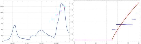
Figure 1.
Estimated CDF (red, thick line) versus the empirical CDF (blue, dashed line) for COVID-19 case data in Ankara.
The dataset in Figure 1 highlights the number of weekly reported cases, showing significant fluctuations over time that correspond to various waves of the pandemic in the region. The first major spike in cases occurs around April 2021, with case numbers rapidly rising, peaking at over 500 cases per week. This surge likely reflects the combined effects of loosened restrictions and increased virus transmissibility. After the peak, there is a gradual decline, followed by a relatively low transmission period through the summer of 2021. The data show a second wave of increasing case numbers starting around October 2021, leading to a sharp spike in early 2022, with a peak in January 2022 where cases exceed 1200 per week. This second wave is likely attributed to the Omicron variant, which is known for its high transmission rate and rapid spread during that period. The significant drop in case numbers by the end of March 2022 reflects the success of public health interventions such as vaccination campaigns, social distancing measures, and possibly the natural decline following the wave. On the right side of Figure 1, we observe the CDF fitted to the data using a Weibull distribution with parameters , , and a location parameter . The Weibull distribution is commonly used in epidemiology and reliability analysis, offering flexibility to model different types of data with increasing or decreasing hazard rates. In this case, the fitted CDF shows a smooth curve, rising sharply around the 40th week (October 2021), which aligns with the timing of the second major wave. The curve levels off after approximately 60 weeks, indicating the slowdown of the pandemic’s progression after the large peak.
The CDF curve reflects the cumulative proportion of cases that have occurred over time. A Weibull distribution with these specific parameters suggests that the spread of COVID-19 in Ankara followed a rapid escalation pattern during each wave, with most cases accumulating during the peaks. The parameters of the Weibull distribution show that the characteristic scale of the spread () and the shape parameter () indicate a distribution where the rate of case increase was sharp but the tail (decline) was less pronounced. This aligns with the observation of rapid case increases during the peaks and a more gradual reduction in cases thereafter.
In Figure 2, the time series of COVID-19 cases in Istanbul and fitted CDF function are depicted.
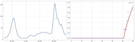
Figure 2.
Estimated CDF (red, thick line) versus the empirical CDF (blue, dashed line) for COVID-19 case data in Istanbul.
The data in Figure 2 illustrate two distinct waves of infection, with the first major peak occurring in April 2021. During this period, the number of weekly reported cases surged to over 1000 cases, indicating the rapid spread of the virus in the densely populated urban environment of Istanbul. The wave eventually subsides by mid-year as public health measures and interventions likely slowed down the transmission. Following a relatively stable and lower period of case numbers throughout the summer and fall of 2021, the second wave begins around December 2021, culminating in a significant peak in January 2022. This second wave coincides with the global spread of the Omicron variant, known for its higher transmissibility. The peak reaches its highest point during this period, with more than 1500 weekly cases recorded. After January 2022, case numbers start to decline sharply, suggesting the impact of vaccinations, immunity development, and the possible effects of natural epidemic burnout. On the right side of Figure 2, the CDF fitted to the data is shown using a Weibull distribution with parameters , , and . The fitted CDF demonstrates how the total number of cases accumulates over time, with the steepest rise occurring around the 50th week. This period aligns with the second peak in January 2022, indicating that the bulk of the cases occurred during this time. The shape parameter suggests that the case distribution has a heavy tail, meaning the cases accumulate quickly once they start, but the decline afterward is relatively gradual. The scale parameter represents the characteristic timescale of the epidemic spread in Istanbul, while the location parameter aligns the distribution with the onset of case accumulation. The sharp rise in the CDF near the end of the observed period is indicative of the rapid growth phase during the second wave, with the steep decline afterward reflecting a rapid drop-off in cases as public health measures took effect.
In Figure 3, the time series of COVID-19 cases in Izmir and fitted CDF function are depicted.
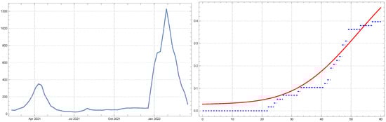
Figure 3.
Estimated CDF (red, thick line) versus the empirical CDF (blue, dashed line) for COVID-19 case data in Izmir.
The data in Figure 3 capture two notable waves of infection. The first wave occurs around April 2021, where case numbers rise sharply, peaking at approximately 400 cases per week before a gradual decline through the middle of the year. This wave corresponds to a period where case numbers across Turkey were rising, likely driven by increased mobility, social interactions, and possibly emerging new variants. The case numbers remained relatively low throughout the summer and fall of 2021, followed by a second and larger wave starting in December 2021 and peaking in January 2022, when weekly cases soared to over 1200. This second wave coincides with the spread of the Omicron variant, a highly transmissible strain that led to significant spikes in cases globally, including Izmir. Following the January peak, the case numbers began to drop rapidly, reflecting the effects of public health interventions and increasing levels of immunity within the population. The right side of Figure 3 displays the CDF fitted to the COVID-19 data using a mixture distribution model. The fitted distribution is a mixture of two normal distributions, with weights 0.620358 and 0.379642. The first component of the mixture is a normal distribution with parameters and , while the second component is another normal distribution with parameters and .
The two-component model suggests that the data can be understood as arising from two distinct phases or groups of events. The first component, centered around 52 weeks, corresponds to the initial wave of cases in April 2021, with a relatively sharp peak and smaller spread (lower variance). This phase reflects the rapid rise and fall of the first wave. The second component, centered around 494 weeks, corresponds to the more sustained and larger wave of infections that peaked in January 2022. This second component has a much wider spread, reflecting the prolonged and more variable nature of the second wave, possibly influenced by the Omicron variant and various public health measures that were implemented in response to the increased transmission. The mixture of two normal distributions in the fitted CDF suggests that the pandemic’s progression in Izmir can be seen as the result of two major waves of differing magnitudes and characteristics. The CDF rises gradually at first, reflecting the early wave, and then accelerates as it incorporates the larger second wave. The weighting of the two components indicates that the second wave had a more substantial impact on the total case count than the first.
For Ankara, the Hurst exponent is 0.4222, indicating anti-persistent behavior. This suggests that the COVID-19 case dynamics in Ankara show a tendency to return to the mean after deviations. In practical terms, this means that when the number of cases increases, it is likely to be followed by a period of decline or stabilization, and vice versa. This behavior might reflect the effectiveness of responsive public health interventions, such as lockdowns and social distancing measures, that were implemented when cases began to surge. The anti-persistence suggests that the pandemic waves in Ankara were more controlled, with spikes in cases quickly followed by mitigation measures that brought the numbers down.
For Istanbul, the Hurst exponent is 0.1932, which is significantly lower than 0.5, indicating strong anti-persistence. This means that the COVID-19 cases in Istanbul exhibited rapid fluctuations, with increases in cases often followed by sharp declines and vice versa. This behavior may be attributed to the high population density and mobility in Istanbul, which likely contributed to the rapid spread of the virus during outbreaks but also to the effectiveness of strict measures, such as targeted lockdowns or restrictions, that were implemented to bring case numbers down quickly. The low Hurst exponent suggests that the city experienced pronounced and frequent oscillations in case numbers, possibly reflecting the challenges of maintaining long-term suppression of the virus in such a large and densely populated urban area.
For Izmir, the Hurst exponent is 0.6085, indicating persistent behavior. This value suggests that the COVID-19 case dynamics in Izmir exhibited longer-term trends, with increases in cases more likely to be followed by further increases. In other words, when cases started to rise in Izmir, the trend was likely to continue for a period before reversing. This persistent behavior could be related to factors such as delayed or less frequent interventions, or the gradual spread of the virus in different waves. The persistence in the case data could also reflect structural factors such as the regional healthcare system’s response or the demographic and social behaviors of the population, which may have contributed to slower reversals in case trends.
The COVID-19 case datasets for Ankara, Istanbul, and Izmir are highly suitable for the proposed model, which aims to capture the spatial and temporal dynamics of infection waves using advanced statistical distributions and fractional differential equations. The data provide detailed weekly case counts over a significant period (February 2021 to March 2022), encompassing two major waves of infections in all three cities. The variability in the timing, intensity, and duration of these waves across different cities makes the dataset ideal for modeling both the local and regional behavior of the pandemic. Each city’s dataset reflects the unique social, demographic, and geographic factors that influenced the spread of the virus, making it possible to study the effects of interventions, population density, and mobility patterns on case trajectories. The presence of distinct waves, especially with differing magnitudes in the second wave (largely driven by the Omicron variant), aligns well with the model’s ability to handle non-linear growth patterns, exponential-like surges, and gradual declines using fractional derivatives and cumulative distribution functions.
The use of Weibull and mixture normal distributions to fit the cumulative distribution functions (CDFs) for these datasets further validates the suitability of the data for the model. These statistical tools allow for an accurate representation of the progression of the pandemic, capturing both early waves with sharper peaks and more prolonged later waves with wider distributions. The model’s ability to incorporate fractional orders derived from the Hurst exponent also benefits from the detailed temporal resolution of the data, which captures the memory effects and long-term dependencies typical of infectious disease dynamics. The variation in the Hurst exponents across the three cities highlights the regional differences in COVID-19 spread and the corresponding public health responses. Istanbul, with the lowest Hurst exponent, experienced the most volatile and unpredictable case dynamics, likely driven by the challenges of managing the virus in such a densely populated urban environment. Ankara, with a Hurst exponent closer to 0.5, showed moderate anti-persistence, reflecting more controlled fluctuations in case numbers. Finally, Izmir exhibited persistent behavior, suggesting that case trends were more prone to continue in the same direction for longer periods, possibly reflecting more gradual waves of infection.
3.2. Results on Numerical Solutions
In this subsection, the results from the numerical solution of the COVID-19 case fractional model for Ankara, Istanbul, and Izmir are presented. The model is based on a set of fixed parameters that define the spatial and temporal domains, as well as the resolution of the spatial and time grids. These fixed parameters are defined as follows: the number of spatial grid points and the number of time grid points , which provide high-resolution data in both the spatial and temporal domains. The spatial domain length and the time domain length are normalized for simplicity, ensuring that the results are easily interpretable. The Gaussian forcing is centered at in the spatial domain and at in the time domain, representing a symmetric application of external influences in both space and time. The amplitude of the Gaussian forcing is fixed at , controlling the intensity of the external influence applied to the system.
To explore how different spatial and temporal spreads of the Gaussian forcing affect the results, three distinct scenarios, varying the spatial () and temporal () spreads are analyzed. Each of these scenarios reflects a different interpretation of how the external forces (such as outbreaks or interventions) might influence the spread of the virus across space and time.
In the first scenario, a relatively small spatial spread and a large temporal spread are chosen. A small spatial spread indicates that the external influence, such as a surge in cases, is confined to a specific part of the spatial domain, reflecting a localized outbreak. The larger temporal spread suggests that this influence persists over an extended period, meaning the external factor (such as a prolonged lockdown or a long-term public health intervention) affects the region gradually over time. This configuration could represent a situation where a localized outbreak, perhaps in a specific neighborhood or district, is managed with sustained intervention. The small spatial spread models the idea that certain areas are more affected than others, while the large temporal spread reflects the necessity of a prolonged response to fully bring the outbreak under control. Such a scenario is relevant in regions where the virus might not spread uniformly but where specific hotspots require extended attention.
In the second scenario, both the spatial and temporal spreads are set to medium values, and . These balanced values indicate that the external influence impacts a broader portion of the spatial domain while also persisting for a considerable, but not overly extended, period of time. A moderate spatial spread suggests that the external factor affects a larger area, such as an entire city or district, while a moderate temporal spread means that the surge in cases or the intervention happens over a typical timeframe, neither too short nor too long. This setup could model the case dynamics in a city-wide outbreak, where the spread of the virus affects multiple regions simultaneously and a coordinated public health response, such as a general lockdown or a vaccination campaign, is applied over several weeks. This configuration captures a situation where the virus is spreading widely but can still be controlled within a moderate timeframe, a scenario that many cities worldwide have faced during different waves of the pandemic.
In the third scenario, a large spatial spread and a small temporal spread are chosen. A large spatial spread means that the external influence affects nearly the entire spatial domain, representing a widespread outbreak or a large-scale public health intervention. The small temporal spread, however, indicates that this intervention or surge in cases is short-lived, suggesting a sudden but brief event, such as a targeted circuit breaker lockdown or a rapid, short-term increase in cases. This scenario could reflect a situation where the virus spreads quickly across a wide area, or where public health measures are applied uniformly across a broad region for a short period of time. The large spatial spread models the simultaneous application of interventions or the widespread nature of a surge, while the small temporal spread reflects a brief but intensive effort to control the outbreak. This configuration is particularly relevant in scenarios where authorities respond decisively with short-term but widespread interventions to quickly curb the spread of the virus.
Figure 4 presents the numerical solutions of the fractional model applied to the COVID-19 case data for Ankara, using different combinations of spatial and temporal spread values for the Gaussian forcing. Each row represents a different combination of the spatial spread and the temporal spread , with the left column showing the 3D surface plots of the solutions and the right column displaying the corresponding density plots.
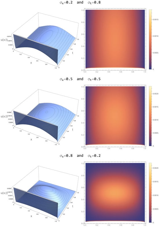
Figure 4.
Numerical solutions of the fractional model applied to the COVID-19 case data for Ankara.
In the first row, the Gaussian forcing parameters are set to and , meaning the spatial influence of the forcing is relatively localized while its temporal effect persists over a longer period. The 3D surface plot on the left shows a smooth and elongated spread across time, with a gradual decrease in the solution’s values as we move away from the center of the domain. This indicates that the external factor, perhaps reflecting a long-term intervention such as a lockdown, has a sustained impact over time but is spatially restricted. The density plot on the right confirms this, with a more concentrated region of influence in the center of the domain, while the effects taper off near the boundaries. This combination suggests that while the intervention or outbreak is spatially confined, it significantly affects the system over an extended period, modeling scenarios where long-term but localized measures are implemented.
In the second row, both the spatial and temporal spreads are set to and , indicating a more balanced distribution of the Gaussian forcing across both space and time. The 3D plot on the left shows a more uniform solution across both dimensions, with a rounded peak in the center of the domain. The density plot on the right reinforces this, with the effects of the forcing distributed relatively evenly across the space-time domain. This suggests that the external factor, likely a moderate and well-distributed intervention, affects a broader region and lasts for a considerable period, but without extreme localization in either space or time. This configuration may represent city-wide interventions such as general lockdowns or widespread vaccination campaigns, where the impact is evenly distributed across both space and time.
In the third row, the spatial spread is large () and the temporal spread is small (), indicating a wide-reaching spatial effect but one that occurs over a short duration. The 3D plot shows a sharp and narrow peak in time, with a rapid rise and fall in the solution, while the spatial extent is more spread out. The density plot supports this observation, showing a broader area of influence in space but with less persistence in time. This combination models a scenario where a large-scale intervention is applied for a brief period, such as a short-term city-wide lockdown or a sudden surge in cases that is quickly brought under control. The spatial breadth of the forcing covers a larger area, indicating a more uniform application of the intervention across the city, but its short duration suggests a more immediate response to a spike in cases.
Figure 5 displays the numerical solutions of the fractional model applied to the COVID-19 case data for Istanbul. Various combinations of spatial and temporal spread values for the Gaussian forcing were utilized. Each row in the data represents a distinct combination of the spatial spread and the temporal spread . The left column contains 3D surface plots of the solutions, while the right column displays the matching density plots.

Figure 5.
Numerical solutions of the fractional model applied to the COVID-19 case data for Istanbul.
In the first row, the Gaussian forcing is characterized by a small spatial spread () and a large temporal spread (). The 3D surface plot on the left shows a smooth, elongated curve, where the effect of the Gaussian forcing is more pronounced over time, and it declines gradually as time progresses. This indicates that the external factor, possibly representing a long-term intervention, such as a lockdown or public health measure, has a prolonged effect over time but is confined spatially to a small portion of the domain. The density plot on the right supports this, showing that the influence is focused in a central region of the spatial domain, with a slower decay over time. This configuration models a scenario where a localized outbreak in a part of Istanbul is managed with long-lasting interventions, representing a sustained response to a concentrated hotspot that persists over time.
The second row shows the results for moderate spatial and temporal spreads (, ). The 3D surface plot displays a more uniform solution, with the peak appearing centered in both space and time. The density plot on the right illustrates a broader spread across the entire domain, indicating that the external influence is more balanced between space and time. This configuration reflects a scenario where the external factor, such as a city-wide intervention, impacts a broader region of Istanbul and persists for a moderate duration. The balanced spread of the forcing in both space and time suggests that this model captures the effects of general lockdowns or public health measures that are neither too localized nor too short-lived, affecting larger regions and lasting for a reasonable period to control the spread of the virus across the city.
The third row presents the results for a large spatial spread () and a small temporal spread (). In this case, the 3D surface plot shows a sharp peak that decays quickly in time but spreads broadly across the spatial domain. The density plot highlights a wide spatial influence, indicating that the external factor impacts almost the entire spatial domain but only for a brief period. This configuration models a scenario where a widespread, short-term intervention is applied across the city. Such a scenario could represent a circuit breaker lockdown or a brief but extensive public health measure implemented to quickly reduce a surge in cases. The short temporal spread suggests that the intervention is rapid, while the large spatial spread shows that the impact is felt uniformly across Istanbul.
Figure 6 exhibits the numerical solutions of the fractional model employed to analyze the COVID-19 case data for Izmir. Different combinations of spatial and temporal spread parameters for the Gaussian forcing are used. Every row in the data corresponds to a unique combination of the spatial spread and the temporal spread . The left column showcases 3D surface plots of the solutions, whereas the right column exhibits the corresponding density plots.
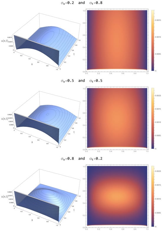
Figure 6.
Numerical solutions of the fractional model applied to the COVID-19 case data for Izmir.
The Gaussian forcing in the first row is defined by a narrow spatial distribution () and a wide temporal distribution (). The 3D surface plot demonstrates a progressive and elongated dispersion over time, characterized by a smooth decline in the value of the solution as time advances. The limited spatial distribution shows that the Gaussian forcing, which represents the external impact on the dynamics of COVID-19, is confined to a certain region within the spatial domain. Conversely, the significant temporal distribution suggests that this impact continues over a prolonged duration. This pattern may indicate a small outbreak in Izmir that is being controlled with enduring public health actions. The density plot verifies this observation by displaying a clustering of influence at the middle of the spatial domain. This influence gradually diminishes with time, indicating the long-lasting presence of the external factor in the temporal dimension. This setup simulates situations in which a certain area of the city has continuous intervention, while the remainder of the city is mostly unaffected.
The second row displays the outcomes with moderate spatial and temporal spreads (, ), providing an equitable distribution of the Gaussian forcing over both space and time. The 3D surface plot exhibits a prominent peak positioned in close proximity to the center of both the spatial and temporal domains. Furthermore, the solution is evenly distributed throughout the whole domain. The density map on the right side displays a homogeneous distribution of influence across both dimensions, indicating that the external factor impacts a larger area of the spatial domain for a moderate period of time. This configuration refers to a public health intervention that is implemented throughout an entire city, such as widespread lockdowns or vaccination programs. These interventions are applied uniformly to the entire population and are maintained for a suitable duration. The use of balanced forcing parameters enables the model to accurately represent the dynamics of broad interventions, demonstrating their simultaneous effects on several areas of Izmir over time.
The Gaussian forcing in the third row is characterized by a significant spatial spread () and a minor temporal spread (). This configuration leads to a concentrated peak in time but a broad geographic impact. The 3D surface plot demonstrates a rapid oscillation in the solution over time, accompanied by a wide distribution over the spatial domain. The density map reveals a significant spatial influence but limited temporal persistence, indicating that the external factor immediately and uniformly affects the entire city but only for a short duration. This setup simulates situations such as a brief yet comprehensive intervention at the city level, where stringent but temporary procedures (such as a “circuit breaker” lockdown or a swift public health response) are implemented throughout Izmir to reduce the impact of a sudden increase in cases. The extensive spatial distribution indicates that the intervention has a broad reach, impacting all regions, while the limited temporal distribution signifies the rapidity of the response.
4. Discussion
The numerical solutions for the fractional model applied to COVID-19 cases in Ankara, Istanbul, and Izmir reveal important differences in the dynamics of virus transmission and the varying impact of public health interventions across these three major Turkish cities. These solutions underscore how spatial and temporal characteristics of the pandemic evolved uniquely in each city, reflecting the distinct demographic, geographic, and mobility patterns, as well as differences in the nature and effectiveness of intervention measures.
In Ankara, the solutions indicate a more localized and gradual response, particularly with smaller spatial spreads. This suggests that targeted interventions or localized outbreaks had a more sustained influence over time, potentially due to more concentrated public health responses or regional variations in the spread of the virus. Ankara’s dynamics appear to reflect a more controlled environment, where localized efforts could better mitigate spikes in cases.
In contrast, the results for Istanbul show significantly more volatility and broader spatial and temporal spreads, indicative of a more complex and widespread response. As Turkey’s largest and most densely populated city, Istanbul experienced more pervasive and rapid fluctuations in case numbers. The larger spatial and temporal spreads reflect the scale and complexity of managing a highly mobile population, where city-wide interventions were necessary to tackle the virus, leading to a more dispersed and prolonged response compared to Ankara. Istanbul’s dynamics capture the challenges of mitigating the spread in a sprawling urban landscape with high population density and extensive social interaction.
For Izmir, the numerical solutions suggest a balance between localized interventions and city-wide responses. The large spatial spreads in some configurations reflect the broader geographic impact of the virus, indicative of a virus that affected multiple regions simultaneously. At the same time, the short temporal spreads suggest that rapid and decisive interventions were employed to control sudden surges in cases, allowing for swift containment measures. The results from Izmir capture a scenario where the virus was widely dispersed, but the response was quick and effective, allowing for localized surges to be controlled in a timely manner.
Overall, the solutions reflect how each city, shaped by varying population densities, urban structures, and public health strategies, responded uniquely to the pandemic. Ankara demonstrates more localized control, reflecting targeted, perhaps more sustained interventions. Istanbul showcases the challenges of implementing broad and prolonged measures to manage a highly complex urban population. Meanwhile, Izmir represents a hybrid response, where interventions effectively balanced between rapid action and city-wide measures to curb the spread of the virus. These findings lay the foundation for a more detailed discussion on the statistical and mathematical analyses of the solutions, further exploring the specific dynamics of the pandemic in each city.
In the following subsections, the results of the numerical solution under different Gaussian forcing values are discussed in detail using three key methods: Pointwise Comparison, Norm-Based Comparison, and Fourier analysis. These methods provide a comprehensive framework for evaluating and contrasting the behavior of the solutions across different cities (Ankara, Istanbul, and Izmir) under varying spatial and temporal spreads of Gaussian forcing.
The Pointwise Comparison method examines the differences between the values of the solution at each corresponding space-time point for two cities. Mathematically, this comparison is expressed as:
where and represent the solutions for two different cities at the same spatial and temporal grid points. This pointwise error allows us to observe how the solutions differ locally, particularly for different forcing configurations. Since this method covers all space-time points in the domain, it provides insight into how response of each city to the spread of COVID-19 varies in terms of local dynamics without relying on specific fixed spatial points.
The Norm-Based Comparison provides a global measure of the difference between the solutions across the entire space-time domain. Two key norms are employed: the norm and the norm. The norm (Euclidean distance) quantifies the overall difference between two solutions by calculating
This norm highlights regions where significant differences exist, capturing the overall magnitude of deviations between the solutions. On the other hand, the norm captures the maximum pointwise difference
By calculating both norms across the entire space–time domain, this method allows for a comprehensive assessment of how different Gaussian forcing values influence the global behavior of the solutions for different cities.
For Fourier analysis, specific spatial points are chosen to analyze the frequency characteristics of the solutions over time. Fourier analysis transforms the time series for a fixed spatial point into the frequency domain, allowing us to observe the dominant frequencies in the temporal evolution of the solution. The Fourier transform is defined as
For this analysis, six representative values have been selected from the spatial domain to capture a range of spatial behaviors: , , , , , and . These values cover the left boundary, points near the boundary, the center of the domain, and the right boundary. By selecting such diverse spatial points, Fourier Analysis can reveal how the temporal dynamics differ between these regions, highlighting variations in behavior of the solution at the boundaries versus the center of the spatial domain. This method is particularly valuable in identifying the impact of different Gaussian forcing values on the temporal behavior of the solutions, especially with regard to oscillatory patterns or periodicities.
4.1. Comparisons for and
Table 1 presents the comparisons of the numerical solutions for Gaussian forcing values of and for each city.

Table 1.
Comparison table of the solutions for and .
Starting with the mean pointwise error, which measures the average absolute difference between solution values at corresponding space–time points, the error between Ankara and Istanbul is , indicating a small difference in their respective solutions. Meanwhile, the error between Ankara and Izmir is slightly higher at , while the error between Istanbul and Izmir is . This suggests that the solutions for Ankara and Istanbul are more similar to each other than they are to the solution for Izmir. However, the errors are quite small overall, indicating that while differences exist, the solutions are generally in close agreement under the current Gaussian forcing parameters.
The norm, which measures the overall magnitude of differences between the solutions in a global sense, provides further insight. The norm between Ankara and Istanbul is , and between Ankara and Izmir, it is , showing that the global difference between Ankara and Izmir is more pronounced than between Ankara and Istanbul. The norm between Istanbul and Izmir is , indicating that while the solutions for Istanbul and Izmir are also distinct, they are closer to each other than Ankara is to Izmir in a global sense. These differences suggest that while the overall behaviors of the solutions are similar, Izmir exhibits more distinct global behavior compared to Ankara and Istanbul.
Finally, the norm, which represents the maximum pointwise difference between solutions, indicates the largest localized differences. The maximum difference between Ankara and Istanbul is , while the maximum difference between Ankara and Izmir is , indicating that the largest localized discrepancy occurs between Ankara and Izmir. The norm between Istanbul and Izmir is , suggesting that there are significant localized differences between these cities as well, though not as large as those between Ankara and Izmir.
Overall, the results show that while the solutions for Ankara, Istanbul, and Izmir exhibit small differences in terms of mean pointwise error, there are more notable global and localized differences, particularly between Ankara and Izmir. This reflects that the spread of COVID-19 cases, as captured by the model, behaves similarly between Ankara and Istanbul under the current forcing conditions, but more divergence is seen between Ankara and Izmir, both in terms of overall trends and localized peaks.
Figure 7 presents the Fourier analysis results for the COVID-19 solutions across different cities (Ankara, Istanbul, and Izmir) at six specific spatial points: , , , , , and . Each subplot corresponds to a different , and the Fourier-transformed values of the solutions are plotted against time for each city. This analysis provides insight into the frequency content and temporal behavior of the solutions at different spatial locations.
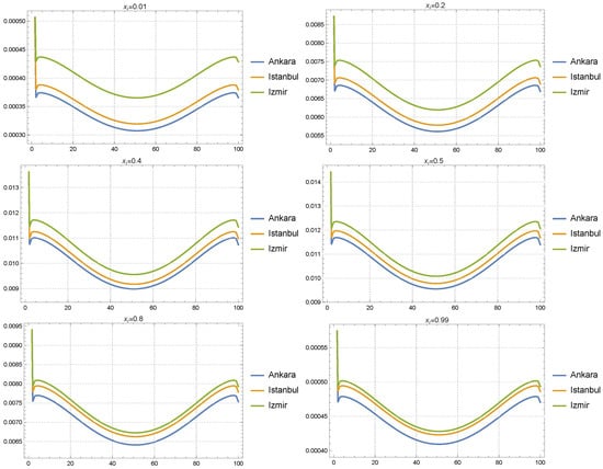
Figure 7.
Fourier analysis results for the COVID-19 solutions across Ankara, Istanbul, and Izmir at six specific spatial points with the Gaussian forcing parameters and .
At the boundaries, particularly at and , the Fourier analysis reveals stronger oscillations at the start of the time domain for all cities, especially for Izmir, followed by Istanbul and then Ankara. The smaller spatial spread of the forcing leads to more localized influences at these boundary points, where the solutions are more sensitive to initial conditions. The larger temporal spread allows the forcing to affect the system over a longer period, which explains the high-amplitude oscillations observed initially. As time progresses, the oscillations diminish across all cities, suggesting that the boundary effects become less significant as the influence of the Gaussian forcing is distributed more evenly throughout the domain. The consistently higher oscillations of Izmir indicate that its solution is more sensitive to boundary effects under these conditions, reflecting a rapid local response. In contrast, solution of Ankara exhibits smoother behavior at the boundaries, indicating a more gradual response to external factors.
In the middle of the domain, at , , , and , the solutions for all three cities show greater convergence, with more uniform and smoother oscillations. At points like and , the differences between the cities become less pronounced. The Fourier analysis at these points shows relatively smaller oscillation amplitudes compared to the boundaries, suggesting that the localized effect of the Gaussian forcing has become more diffused. The extended temporal influence, on the other hand, has resulted in a more stable and consistent evolution of the solutions across all cities. This indicates that as we move away from the boundaries, the effects of the forcing parameters on the solution become more uniform, resulting in similar temporal behaviors between Ankara, Istanbul, and Izmir.
Overall, the Fourier analysis under and reveals that boundary effects are more prominent at the edges of the spatial domain, particularly for Izmir, while the mid-domain behavior is characterized by smoother, more stable oscillations across all three cities. This suggests that the influence of the forcing parameters varies spatially, with stronger localized effects near the boundaries and more uniform dynamics near the center of the domain.
4.2. Comparisons for and
Table 2 presents the comparisons of the numerical solutions for Gaussian forcing values of and for each city.
Table 2.
Comparison table of the solutions for and .
For Ankara and Istanbul, the mean pointwise error is , which is slightly larger than the corresponding value in the previous configuration ( and ). This indicates a small increase in the differences between Ankara and Istanbul’s solutions under this new forcing configuration, though the difference remains minimal overall. The mean pointwise error between Ankara and Izmir is , which is consistent with the previous table, suggesting that the average behavior between these two cities has not been significantly affected by the change in spatial and temporal spreads. Similarly, the mean pointwise error between Istanbul and Izmir is , which also remains stable compared to the earlier configuration. Overall, this metric shows that while there are minor differences between the cities, the solutions remain closely aligned under the new forcing conditions.
The norm between Ankara and Istanbul is , the same as in the previous configuration, indicating that the global differences between these two cities are unaffected by the change in forcing. The norm between Ankara and Izmir is , which also remains unchanged, highlighting a stable and consistent global difference between these cities. The norm between Istanbul and Izmir is , showing that the global difference between these two cities has also remained constant under the new parameters. This consistency in the norm across cities suggests that, globally, the solutions are robust and unaffected by moderate changes in the spatial and temporal spread of the Gaussian forcing.
Between Ankara and Istanbul, the norm is , indicating that the largest local difference between these two cities remains small but unchanged from the previous table. The norm between Ankara and Izmir is , indicating that the largest local differences between these two cities are more substantial, but again, consistent with the previous analysis. The norm between Istanbul and Izmir is , highlighting that the largest local difference between these two cities is moderate and stable across both forcing configurations.
In summary, the comparison table shows that the solutions for Ankara, Istanbul, and Izmir remain consistent in their overall behavior, both globally and locally, under the new forcing parameters of and . While the mean pointwise error and norms reflect minor differences between the cities, these differences are relatively small, indicating that the solutions are closely aligned, even when the spatial and temporal spreads of the Gaussian forcing are adjusted. This stability suggests that the cities’ response to the model’s forcing parameters is robust, with no significant changes in behavior as the parameters vary.
Figure 8 presents the results of the Fourier analysis for Ankara, Istanbul, and Izmir at six different spatial points, , , , , , and , with the Gaussian forcing parameters and . These parameters represent moderate spatial and temporal spreads, reflecting a balance between the localized spatial impact and a more sustained temporal influence.
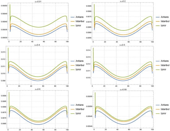
Figure 8.
Fourier analysis results for the COVID-19 solutions across Ankara, Istanbul, and Izmir at six specific spatial points with the Gaussian forcing parameters and .
At the boundary points and , all three cities exhibit noticeable oscillatory behavior, with a sharp initial spike at the beginning of the time domain. This is followed by a smoother, periodic oscillation over time. In these regions, Izmir consistently shows larger amplitude oscillations compared to Istanbul and Ankara, indicating a more pronounced response to the boundary conditions. The boundary effects, as represented by the oscillations, suggest that the forcing is having a strong localized impact, particularly for Izmir. This heightened sensitivity at the boundaries reflects the effect of the moderate spatial spread , which still concentrates some influence at the edges of the domain. Meanwhile, Ankara shows the least boundary-induced oscillations, implying a more stable behavior under the same conditions, while Istanbul falls between Ankara and Izmir in terms of sensitivity.
As we move away from the boundaries, at , the oscillatory behavior for all three cities becomes more uniform, though Izmir continues to exhibit slightly higher amplitudes. The general periodic nature of the oscillations suggests that the solutions are stabilizing in this region, with the influence of the Gaussian forcing being more evenly distributed in space and time. This is indicative of the balanced nature of the forcing parameters, which are designed to influence the system without being overly concentrated in any one region. The behavior at reflects a transition zone, where the solutions begin to diverge less from each other, signaling a convergence in the mid-domain.
At the central spatial points, and , the solutions for Ankara, Istanbul, and Izmir show very close alignment. The amplitude differences are minimal, and the oscillations exhibit smooth and periodic patterns across the time domain. This suggests that, in the central regions of the domain, the influence of the Gaussian forcing is well balanced between space and time, leading to a more uniform temporal evolution across all cities. The mid-domain appears to be where the solutions converge most, indicating that the dynamics are largely similar in this region under the current forcing conditions. This uniformity further reinforces the idea that the spatial and temporal spreads are influencing the system in a balanced manner, with less pronounced differences between the cities.
Finally, at , the behavior begins to diverge slightly again, although not as drastically as at the boundaries. Izmir still shows slightly higher oscillation amplitudes compared to Ankara and Istanbul, but the differences remain relatively small. The periodicity is still present, and the solutions continue to behave in a stable, predictable manner, reflecting the moderate spread of the forcing across space and time.
The Fourier analysis across different spatial points shows that the solutions for all three cities exhibit stronger boundary effects, particularly for Izmir, at the edges of the domain, while the mid-domain points show more uniform behavior. The moderate spatial and temporal forcing parameters and allow the solutions to stabilize in the central regions of the domain, where the differences between cities become less pronounced. This suggests that while the boundary regions are more sensitive to the forcing conditions, the central regions of the domain are less affected, leading to more convergence in the solutions for Ankara, Istanbul, and Izmir.
4.3. Comparisons for and
Table 3 presents the comparisons of the numerical solutions for Gaussian forcing values of and for each city.
Table 3.
Comparison table of the solutions for and .
The mean pointwise error measures the average absolute difference between the solutions at corresponding points in space and time. The error between Ankara and Istanbul is , indicating a minimal difference between their solutions under this Gaussian forcing configuration. This error is slightly larger than the previous configurations, suggesting that the broader spatial spread of the forcing has introduced a slightly larger difference between Ankara and Istanbul. The mean pointwise error between Ankara and Izmir is , the same as in previous tables, indicating a stable average behavior in the differences between these two cities. Similarly, the error between Istanbul and Izmir is , also consistent with earlier results. Overall, the mean pointwise error remains small, showing that despite the broader spatial influence of the forcing, the solutions for all three cities remain quite similar.
The norm, which measures the overall global differences between the solutions, provides further insight into the relative differences between the cities. The norm between Ankara and Istanbul is , identical to the previous configurations, indicating that the global differences between these two cities have not been significantly affected by the changes in the Gaussian forcing parameters. The norm between Ankara and Izmir is , also consistent with previous values, suggesting that the broader spatial influence has not altered the global differences between these cities. The norm between Istanbul and Izmir is , showing that the global differences between these two cities have remained stable. The consistency in the norms across the cities highlights that the overall magnitude of the differences is robust to changes in the spatial and temporal spreads of the forcing.
The norm, which captures the maximum pointwise difference between the solutions, reveals more localized differences. Between Ankara and Istanbul, the norm is , indicating that the largest local difference between these two cities remains small but is consistent with previous results. The norm between Ankara and Izmir is , reflecting the largest local difference, which remains stable compared to earlier configurations. The norm between Istanbul and Izmir is , showing that the largest local differences between these two cities have not changed significantly. This consistency suggests that while localized differences exist, the maximum pointwise differences are largely unaffected by the broader spatial spread and shorter temporal influence of the Gaussian forcing.
The comparison table for and shows that the solutions for Ankara, Istanbul, and Izmir remain closely aligned, with minimal changes in the mean pointwise error, norm, and norm compared to other configurations. The broader spatial influence and shorter temporal impact of the Gaussian forcing do not lead to significant changes in the overall behavior of the solutions, indicating that the cities’ responses to the model’s forcing parameters are stable and consistent across different forcing scenarios.
Figure 9 presents the Fourier analysis results for the COVID-19 model applied to Ankara, Istanbul, and Izmir at six different spatial points. The Gaussian forcing parameters for these results are and , representing a broad spatial influence and a shorter temporal effect. This configuration is expected to have a wider spread of influence across the spatial domain but with a more immediate, shorter-lasting impact in time.
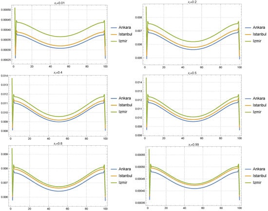
Figure 9.
Fourier analysis results for the COVID-19 solutions across Ankara, Istanbul, and Izmir at six specific spatial points with the Gaussian forcing parameters and .
At the boundary points and , all three cities exhibit noticeable oscillatory behavior, with Izmir consistently showing the highest amplitudes compared to Istanbul and Ankara. This pattern suggests that Izmir’s solution is more sensitive to the boundary conditions, with larger fluctuations near the edges of the spatial domain. The influence of the broader spatial spread can be seen in the way that all three cities experience relatively strong initial oscillations at the boundaries, although Izmir exhibits more pronounced variations. As we move further into the time domain, these oscillations decrease, indicating that the boundary effects dissipate as the influence of the Gaussian forcing becomes more evenly distributed.
At the intermediate points and , the solutions for all three cities become more synchronized. The oscillatory behavior still persists, but the differences between the cities are less pronounced compared to the boundary points. The broader spatial spread of is more evenly distributed across the domain at these points, allowing the solutions to converge more closely in their frequency behavior. Izmir continues to show slightly higher oscillations, reflecting a greater sensitivity to the forcing parameters, but the differences are not as significant as at the boundaries. This indicates that the mid-domain points are less influenced by localized effects and more by the global impact of the forcing.
At the central spatial points and , the solutions for Ankara, Istanbul, and Izmir exhibit very similar behavior. The oscillations are smooth, and the amplitude differences between the cities are minimal. This suggests that, in the central region of the domain, the Gaussian forcing is having a uniform effect across the three cities, with little deviation in their responses. The shorter temporal spread also plays a role here, as the temporal influence of the forcing diminishes quickly, leading to more stable and synchronized behavior across the cities as time progresses.
Overall, the Fourier analysis reveals that while the solutions for Ankara, Istanbul, and Izmir exhibit stronger oscillatory behavior near the boundaries, particularly for Izmir, the central and mid-domain points show more uniformity. The broader spatial spread of ensures that the influence of the Gaussian forcing is distributed across the domain, while the shorter temporal spread results in a more immediate, short-term impact on the solutions. This combination leads to stronger boundary effects but more consistent behavior in the central regions of the spatial domain.
5. Conclusions
In conclusion, this study has presented a fractional advection–diffusion–reaction model for analyzing COVID-19 dynamics in major Turkish cities, demonstrating its ability to capture complex spatial–temporal transmission patterns. Our numerical experiments and statistical analyses reveal that the integration of memory effects—via a Caputo-type fractional derivative determined by the Hurst exponent—enables the model to effectively represent the cumulative influence of past infection waves, incubation delays, and intervention measures. This capability is underscored by our fitted distribution analysis, where the Weibull and mixture normal distributions accurately reflected the distinct epidemic behaviors observed in Ankara, Istanbul, and Izmir. For example, the model captures the more controlled, localized dynamics in Ankara, the volatile and rapidly fluctuating case numbers in Istanbul, and the persistent trends with bimodal characteristics in Izmir, each of which highlights the importance of tailoring public health interventions to the unique urban context.
Our key findings indicate that the model not only reproduces the evolution of the epidemic across different regions but also provides insights into the impact of varying intervention strategies. The sensitivity analysis confirms that parameters such as the fractional order and the temporal spread of the Gaussian forcing have a significant influence on the model outcomes, emphasizing the necessity for precise calibration to capture both the peak intensity and cumulative case burden accurately. These results collectively underscore the model’s enhanced descriptive and predictive capabilities compared to conventional integer-order approaches.
Nevertheless, several limitations warrant further discussion. We acknowledge that the true number of COVID-19 cases is inherently difficult to measure precisely due to factors such as underreporting, limited testing, and delays in reporting. Consequently, our model predictions are treated as approximations that incorporate inherent measurement error and unobserved variability in the transmission process. While the current formulation employs a deterministic framework, it does not explicitly account for random fluctuations or noise inherent in real-world data. Moreover, the implicit finite difference scheme, despite ensuring numerical stability, carries a significant computational cost due to the non-local memory effects of fractional derivatives, which require extensive storage and processing of historical data.
Future work will focus on addressing these limitations by extending the model to incorporate stochastic terms in the reaction and forcing components, thereby allowing for the quantification of uncertainty through confidence intervals or probability distributions. In addition, we plan to investigate optimization strategies—such as fast convolution algorithms, advanced memory management, parallel computing, and adaptive discretization techniques—to enhance computational efficiency and scalability. These improvements will not only refine the predictive accuracy of the model but also facilitate its application to larger datasets and potential real-time forecasting scenarios.
Overall, our study lays the groundwork for a more nuanced and adaptable modeling framework that advances the understanding of COVID-19 dynamics in diverse urban environments while also identifying clear pathways for future research to overcome current limitations and further improve model performance.
Author Contributions
Conceptualization, L.M.B., D.A.K., Ö.A., M.A.B. and A.N.; methodology, L.M.B., D.A.K., Ö.A., M.A.B. and A.N.; software, Ö.A. and M.A.B.; validation, D.A.K., Ö.A., M.A.B., L.M.B. and A.N.; formal analysis, L.M.B., D.A.K., Ö.A., M.A.B. and A.N.; investigation, L.M.B., D.A.K., Ö.A., M.A.B. and A.N.; resources, L.M.B., D.A.K., Ö.A., M.A.B. and A.N.; data curation, L.M.B. and A.N.; writing—original draft preparation, L.M.B., D.A.K., Ö.A., M.A.B. and A.N.; writing—review and editing, L.M.B., D.A.K., Ö.A., M.A.B. and A.N.; visualization, Ö.A. and M.A.B.; supervision, M.A.B.; project administration, A.N.; funding acquisition, A.N. All authors have read and agreed to the published version of the manuscript.
Funding
This research received no external funding.
Data Availability Statement
The original contributions presented in the study are included in the article; further inquiries can be directed to the corresponding authors.
Conflicts of Interest
The authors declare no conflicts of interest.
Appendix A. Model Sensitivity Analysis
Figure A1 illustrates how the model’s peak value and area under the curve (AUC) depend on variations in both the fractional order and the temporal spread.
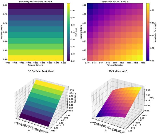
Figure A1.
Sensitivity analysis of the peak value and area under the curve (AUC) with respect to the fractional order and the temporal spread.
In the top row, the heatmaps show that small changes in either or can lead to noticeable shifts in these output metrics, with warmer colors indicating higher values of peak or AUC. The peak value heatmap suggests a gradual gradient along both axes, reflecting how the system’s maximum intensity is influenced by the interplay between the memory effect captured by and the duration of external forcing represented by . The AUC heatmap follows a similar pattern, but the transition in color shades appears more uniform, implying that cumulative disease spread is moderately sensitive to both parameters without exhibiting sharp discontinuities. The 3D surface plots in the bottom row confirm these observations and provide a clearer visual perspective of the model’s sensitivity. As increases, the memory effect intensifies, potentially prolonging the influence of past infection levels and elevating the peak value. Meanwhile, increases in cause the forced intervention or outbreak duration to expand, which can amplify both the peak and the total area under the curve. The surfaces exhibit smooth gradients rather than abrupt jumps, indicating that the model responds in a relatively continuous fashion to parameter changes.
Figure A2 illustrates how variations in the forcing amplitude A affect both the peak value and the total area under the curve of the model’s output.
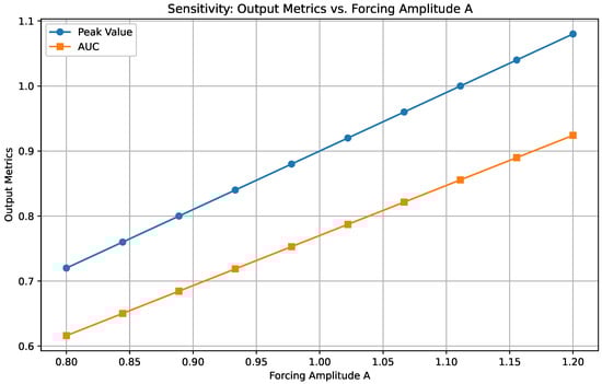
Figure A2.
Sensitivity analysis of the peak value and area under the curve (AUC) with respect to the forcing amplitude A.
As A increases, the peak value (blue line) rises steadily, indicating that stronger external forcing leads to higher maximum infection levels. The AUC (orange line) also exhibits a consistent upward trend, suggesting that a more intense forcing not only raises the infection peak but also extends its overall impact. This linear relationship in both metrics highlights the direct influence of the amplitude parameter on the model’s dynamics. In practical terms, a larger forcing amplitude may correspond to either a more severe outbreak or a more aggressive intervention scenario, both of which amplify the cumulative effect of the model over time.
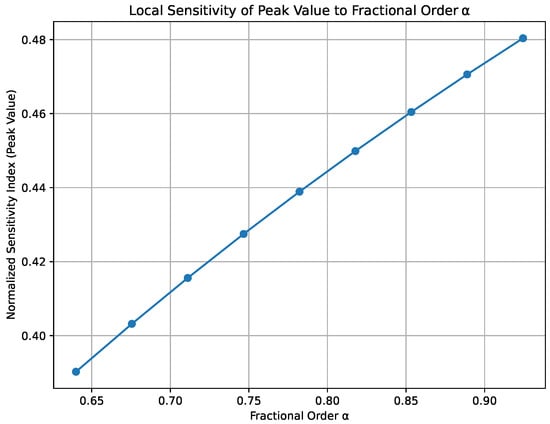
Figure A3.
Local sensitivity of the peak value to the fractional order .
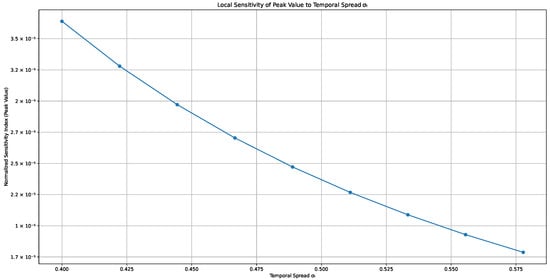
Figure A4.
Local Local sensitivity of the peak value to the temporal spread .
As increases, the index rises steadily, indicating that small changes in the memory effect can substantially alter the model’s maximum infection level. This trend underscores the importance of accurately estimating , since it modulates how strongly past infection levels influence the current state. A higher sensitivity index suggests that any uncertainty in will translate into greater uncertainty in predicting the peak of the epidemic curve, highlighting the need for careful calibration of this parameter.
The plot focuses on the local sensitivity of the peak value to variations in the temporal spread . Here, the index shows a gradual decrease with increasing , implying that the system becomes less sensitive to incremental changes in the duration of the forcing as grows. Although the memory effect still plays a role, the model’s maximum infection level appears less responsive to further widening of the temporal window once reaches moderate or high values. Consequently, this behavior indicates that while initial expansions of may strongly affect the peak, further broadening of the forcing duration yields diminishing returns in altering the model’s peak dynamics.
Appendix B. Distribution Fit Analysis
In order to determine the underlying distribution that best describes our (discrete) COVID-19 data, we employ a kernel density estimation (KDE) approach to generate a smooth probability density function over the observed values. Let denote the discrete data points, which we treat as realizations on a continuum for the sake of density estimation. The KDE is defined by
where is the chosen kernel function (for our case, a Gaussian kernel), and h is the bandwidth parameter that controls the degree of smoothing. Despite the discrete nature of the data, this procedure yields a continuous approximation of the underlying probability distribution by assigning mass around each observed data point in a controlled manner. We then evaluate the resulting KDE-based fit against candidate distributions—such as Weibull, Pareto, or normal mixtures—using information criteria and goodness-of-fit metrics (e.g., Chi Square or Cramer–Von Mises) to ascertain which distribution provides the most accurate representation of the empirical data. The top three distributions fitted to each city data are analyzed in Table A1.
Table A1.
Top 3 distributions fitted into COVID-19 data for each city.
Table A1.
Top 3 distributions fitted into COVID-19 data for each city.
| Ankara | Istanbul | Izmir | |||||||
|---|---|---|---|---|---|---|---|---|---|
| Top 1 | Top 2 | Top 3 | Top 1 | Top 2 | Top 3 | Top 1 | Top 2 | Top 3 | |
| Fitted Distribution | Weibull | Pareto | Log Normal | Weibull | Pareto | Log Normal | Normal and Normal | Gamma and Normal | Log Normal and Normal |
| Chi Square | 0.273683 | 0.00017 | 0.449616 | 0.249826 | 0.005965 | 0.138475 | 0.187624 | 0.00013 | 0.090177 |
| Cramer−von Mises | 0.344002 | 0.004108 | 0.965361 | 0.564084 | 0.005846 | 0.710442 | 0.467984 | 0.47291 | 0.525633 |
| BIC | −13.3725 | −13.5103 | −13.5607 | −13.4381 | −13.5578 | −13.7062 | −12.0503 | −11.9417 | −12.0159 |
| AIC | −13.3687 | −13.508 | −13.5568 | −13.4342 | −13.5555 | −13.7062 | −12.051 | −11.9424 | −12.0166 |
| HQIC | −13.4025 | −13.5503 | −13.5807 | −13.4681 | −13.5978 | −13.7301 | −12.1003 | −11.9917 | −12.0659 |
| Log Likelihood | −6.62879 | −6.67851 | −74202 | −6.66155 | −6.70226 | −6.81675 | −5.92933 | −5.87507 | −5.91214 |
| Complexity | 3 | 4 | 2 | 3 | 4 | 2 | 5 | 5 | 5 |
| Error | 6.62879 | 6.67851 | 6.74202 | 6.66155 | 6.70226 | 6.81675 | 5.92933 | 5.87507 | 5.91214 |
| Internal | −13.4972 | −13.6586 | −13.6881 | −13.5627 | −13.7061 | −13.8375 | −12.09997 | −13.1514 | −12.1905 |
For Ankara, the Weibull distribution emerges as the top choice because it balances a solid statistical fit with interpretability and manageable complexity. Although the Pareto model shows extremely low Chi Square and Cramer–Von Mises values, the Weibull distribution offers parameters that are more directly interpretable in the context of epidemiological dynamics and reliability analysis. Its competitive AIC, BIC, and HQIC values underscore that it fits the data well without overcomplicating the model, making it a pragmatic choice for capturing the spread and decline patterns observed in Ankara’s COVID-19 case data.
For Istanbul, the Weibull distribution is also identified as the best fit among the candidate models. Its fit metrics, such as a relatively low Chi Square value and competitive information criteria (AIC, BIC, and HQIC), indicate that it effectively captures the underlying distribution of the data. The Weibull model’s flexibility allows it to account for the variability and tail behavior inherent in Istanbul’s epidemiological trends, while maintaining a low model complexity. This balance is particularly valuable in a densely populated urban setting where the dynamics of disease transmission can be intricate, yet require a model that is both robust and interpretable.
For Izmir, the normal and normal mixture model is selected as the top fitted distribution due to its superior ability to capture the heterogeneous nature of the data. Unlike a single distribution, the dual-component model reflects the presence of multiple underlying processes—possibly corresponding to distinct waves or clusters of cases—that a single distribution might overlook. With a lower Chi Square value and competitive AIC and BIC despite its higher complexity, this mixture model provides a nuanced representation of the data. Its capacity to model bimodal or multimodal behavior makes it particularly suitable for Izmir, where the epidemic dynamics appear more complex and variable compared to the other cities.
References
- Diagne, M.; Rwezaura, H.; Tchoumi, S.; Tchuenche, J. A mathematical model of COVID-19 with vaccination and treatment. Comput. Math. Methods Med. 2021, 2021, 1250129. [Google Scholar] [PubMed]
- Kouidere, A.; Khajji, B.; El Bhih, A.; Balatif, O.; Rachik, M. A mathematical modeling with optimal control strategy of transmission of COVID-19 pandemic virus. Commun. Math. Biol. Neurosci. 2020, 2020, 24. [Google Scholar]
- Wang, N.; Fu, Y.; Zhang, H.; Shi, H. An evaluation of mathematical models for the outbreak of COVID-19. Precis. Clin. Med. 2020, 3, 85–93. [Google Scholar] [PubMed]
- Xiang, Y.; Jia, Y.; Chen, L.; Guo, L.; Shu, B.; Long, E. COVID-19 epidemic prediction and the impact of public health interventions: A review of COVID-19 epidemic models. Infect. Dis. Model. 2021, 6, 324–342. [Google Scholar] [PubMed]
- Guglielmi, N.; Iacomini, E.; Viguerie, A. Delay differential equations for the spatially resolved simulation of epidemics with specific application to COVID-19. Math. Methods Appl. Sci. 2022, 45, 4752–4771. [Google Scholar]
- Kevrekidis, P.; Cuevas-Maraver, J.; Drossinos, Y.; Rapti, Z.; Kevrekidis, G. Reaction-diffusion spatial modeling of COVID-19: Greece and andalusia as case examples. Phys. Rev. E 2021, 104, 024412. [Google Scholar]
- Mammeri, Y. A reaction-diffusion system to better comprehend the unlockdown: Application of seir-type model with diffusion to the spatial spread of COVID-19 in france. Comput. Math. Biophys. 2020, 8, 102–113. [Google Scholar]
- Schäfer, M.; Heidrich, P.; Götz, T. Modelling the spatial spread of COVID-19 in a german district using a diffusion model. Math. Biosci. Eng. MBE 2023, 20, 21246–21266. [Google Scholar]
- Viguerie, A.; Lorenzo, G.; Auricchio, F.; Baroli, D.; Hughes, T.; Patton, A.; Reali, A.; Yankeelov, T.; Veneziani, A. Simulating the spread of COVID-19 via a spatially-resolved susceptible–exposed–infected–recovered–deceased (seird) model with heterogeneous diffusion. Appl. Math. Lett. 2021, 111, 106617. [Google Scholar]
- Saleem, F.; Al-Ghamdi, A.S.A.M.; Alassafi, M.O.; AlGhamdi, S.A. Machine learning, deep learning, and mathematical models to analyze forecasting and epidemiology of COVID-19: A systematic literature review. Int. J. Environ. Res. Public Health 2022, 19, 5099. [Google Scholar] [CrossRef]
- Afzal, A.; Saleel, C.A.; Bhattacharyya, S.; Satish, N.; Samuel, O.D.; Badruddin, I.A. Merits and limitations of mathematical modeling and computational simulations in mitigation of COVID-19 pandemic: A comprehensive review. Arch. Comput. Methods Eng. 2022, 29, 1311–1337. [Google Scholar] [PubMed]
- Moreau, J. Systematic Review of Mathematical Models for Viral Transmission Dynamics: Insights from COVID-19 Studies. Lett. Biomath. 2024, 11, 21–30. [Google Scholar]
- Peter, S.; Dittrich, P.; Ibrahim, B. Structure and hierarchy of SARS-CoV-2 infection dynamics models revealed by reaction network analysis. Viruses 2020, 13, 14. [Google Scholar] [CrossRef]
- Ibrahim, B.; McMahon, D.P.; Hufsky, F.; Beer, M.; Deng, L.; Le Mercier, P.; Palmarini, M.; Thiel, V.; Marz, M. A new era of virus bioinformatics. Virus Res. 2018, 251, 86–90. [Google Scholar] [PubMed]
- Balci, M. Fractional virus epidemic model on financial networks. Open Math. 2016, 14, 1074–1086. [Google Scholar] [CrossRef]
- Balcı, M. Time fractional capital-induced labor migration model. Phys. A Stat. Mech. Its Appl. 2017, 477, 91–98. [Google Scholar]
- Balcı, M.; Akgüller, Ö.; Batrancea, L.; Nichita, A. The impact of turkish economic news on the fractality of borsa istanbul: A multidisciplinary approach. Fractal Fract. 2023, 8, 32. [Google Scholar] [CrossRef]
- Balcı, M. Distributed order model of labor migration. Int. J. Nonlinear Sci. Numer. Simul. 2023, 24, 2497–2512. [Google Scholar]
- Balcı, M.; Batrancea, L.; Akgüller, Ö.; Gaban, L.; Rus, M.; Tulai, H. Fractality of borsa istanbul during the COVID-19 pandemic. Mathematics 2022, 10, 2503. [Google Scholar] [CrossRef]
- Lombard, F.; Robbertse, J. Testing constancy of the hurst exponent of some long memory stationary gaussian time series. S. Afr. Stat. J. 2012, 46, 247–266. [Google Scholar]
- Von Wegner, F.; Laufs, H.; Tagliazucchi, E. Mutual information identifies spurious hurst phenomena in resting state eeg and fmri data. Phys. Rev. E 2018, 97, 022415. [Google Scholar] [CrossRef] [PubMed]
- Cheng, B.; Wang, Y. A logistic model and predictions for the spread of the COVID-19 pandemic. Chaos Interdiscip. J. Nonlinear Sci. 2020, 30, 123135. [Google Scholar] [CrossRef]
- Pincheira-Brown, P.; Bentancor, A. Forecasting COVID-19 infections with the semi-unrestricted generalized growth model. Epidemics 2021, 37, 100486. [Google Scholar] [CrossRef] [PubMed]
- Ahmed, A.; Rahimian, M.; Roberts, M. Inferring epidemic dynamics using gaussian process emulation of agent-based simulations. In Proceedings of the 2023 Winter Simulation Conference (WSC), San Antonio, TX, USA, 10–13 December 2023; pp. 770–780. [Google Scholar]
- Chen, S.; Xu, J.; Wu, Y.; Wang, X.; Fang, S.; Cheng, J.; Ma, H.; Zhang, R.; Liu, Y.; Zhang, L.; et al. Predicting temporal propagation of seasonal influenza using improved gaussian process model. J. Biomed. Informatics 2019, 93, 103144. [Google Scholar] [CrossRef]
- Park, J.; Yi, S.; Chang, W.; Mateu, J. A spatio-temporal dirichlet process mixture model for coronavirus disease-19. Stat. Med. 2023, 42, 5555–5576. [Google Scholar] [CrossRef] [PubMed]
- Chang, E.; Moselle, K.; Richardson, A. Covidsimvl–transmission trees, superspreaders and contact tracing in agent based models of COVID-19. medRxiv 2020, 2020-12. [Google Scholar]
- Din, A.; Khan, A.; Baleanu, D. Stationary distribution and extinction of stochastic coronavirus (COVID-19) epidemic model. Chaos Solitons Fractals 2020, 139, 110036. [Google Scholar] [CrossRef]
- Saeed, F.; Paul, A.; Ahmed, M. Forecasting COVID-19 cases using multiple statistical models. In Proceedings of the 2020 8th International Conference on Orange Technology (ICOT), Daegu, Republic of Korea, 18–21 December 2020; pp. 1–5. [Google Scholar]
- Bradley, W.; Kim, J.; Kilwein, Z.; Blakely, L.; Eydenberg, M.; Jalvin, J.; Laird, C.; Boukouvala, F. Perspectives on the integration between first-principles and data-driven modeling. Comput. Chem. Eng. 2022, 166, 107898. [Google Scholar] [CrossRef]
- Linkletter, C.; Bingham, D.; Hengartner, N.; Higdon, D.; Ye, K. Variable selection for gaussian process models in computer experiments. Technometrics 2006, 48, 478–490. [Google Scholar] [CrossRef]
- Bondarenko, V.; Mazzega, P.; Lajaunie, C. Predictability of scrub typhus incidences time series in thailand. Eng. Proc. 2021, 5, 44. [Google Scholar] [CrossRef]
- Das, D.; Chowdhury, S.; Das, G.; Chanda, A.; Khamaru, S.; Ghosh, K. A study on self similar, nonlinear and complex behavior of the spread of COVID-19 in India. In Advances in Mathematical Analysis and Its Applications; Chapman and Hall/CRC: New York, NY, USA, 2022; pp. 311–334. [Google Scholar]
- Diebner, H.; Timmesfeld, N. Exploring COVID-19 daily records of diagnosed cases and fatalities based on simple nonparametric methods. Infect. Dis. Rep. 2021, 13, 302–328. [Google Scholar] [CrossRef] [PubMed]
- Samadder, S.; Ghosh, K. Analysis of self-similarity, memory and variation in growth rate of COVID-19 cases in some major impacted countries. J. Phys. Conf. Ser. 2021, 1797, 012010. [Google Scholar]
- Mickens, R. A nonstandard finite difference scheme for a fisher pde having nonlinear diffusion. Comput. Math. Appl. 2003, 45, 429–436. [Google Scholar]
Disclaimer/Publisher’s Note: The statements, opinions and data contained in all publications are solely those of the individual author(s) and contributor(s) and not of MDPI and/or the editor(s). MDPI and/or the editor(s) disclaim responsibility for any injury to people or property resulting from any ideas, methods, instructions or products referred to in the content. |
© 2025 by the authors. Licensee MDPI, Basel, Switzerland. This article is an open access article distributed under the terms and conditions of the Creative Commons Attribution (CC BY) license (https://creativecommons.org/licenses/by/4.0/).