

Fractional-Order Modeling and Identification for Dual-Inertia Servo Inverter Systems with Lightweight Flexible Shaft or Coupling


Abstract
1. Introduction
- (1)
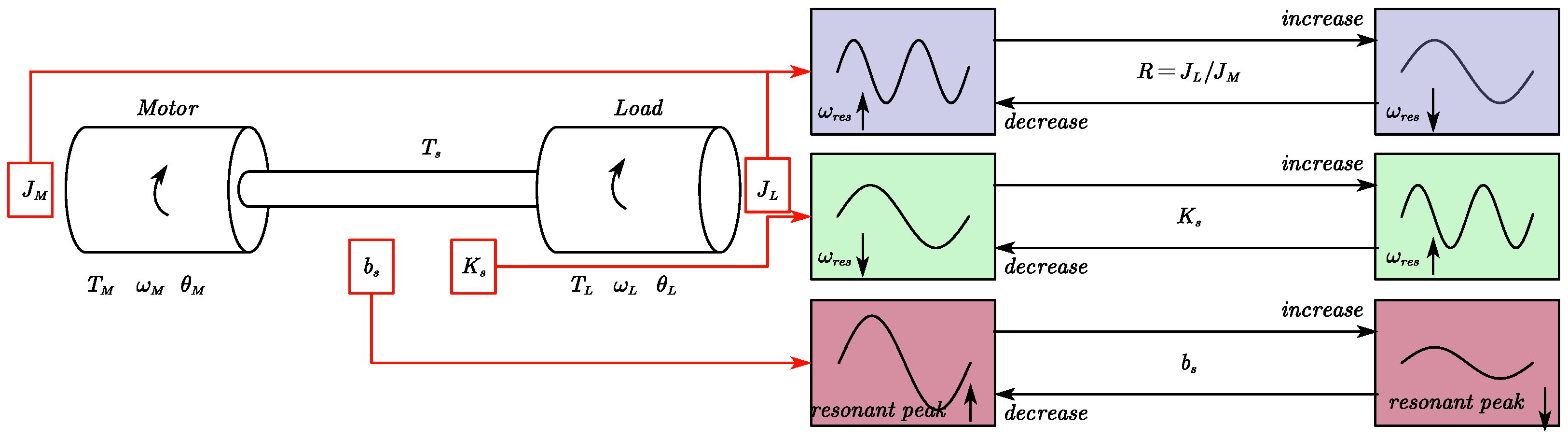
- The structural composition of the dual-inertia system and the mechanisms underlying resonance generation were investigated. The principle of fractional-order calculus was introduced to extend the current model of the dual-inertia system from the integer-order one to the fractional-order one.
- (2)
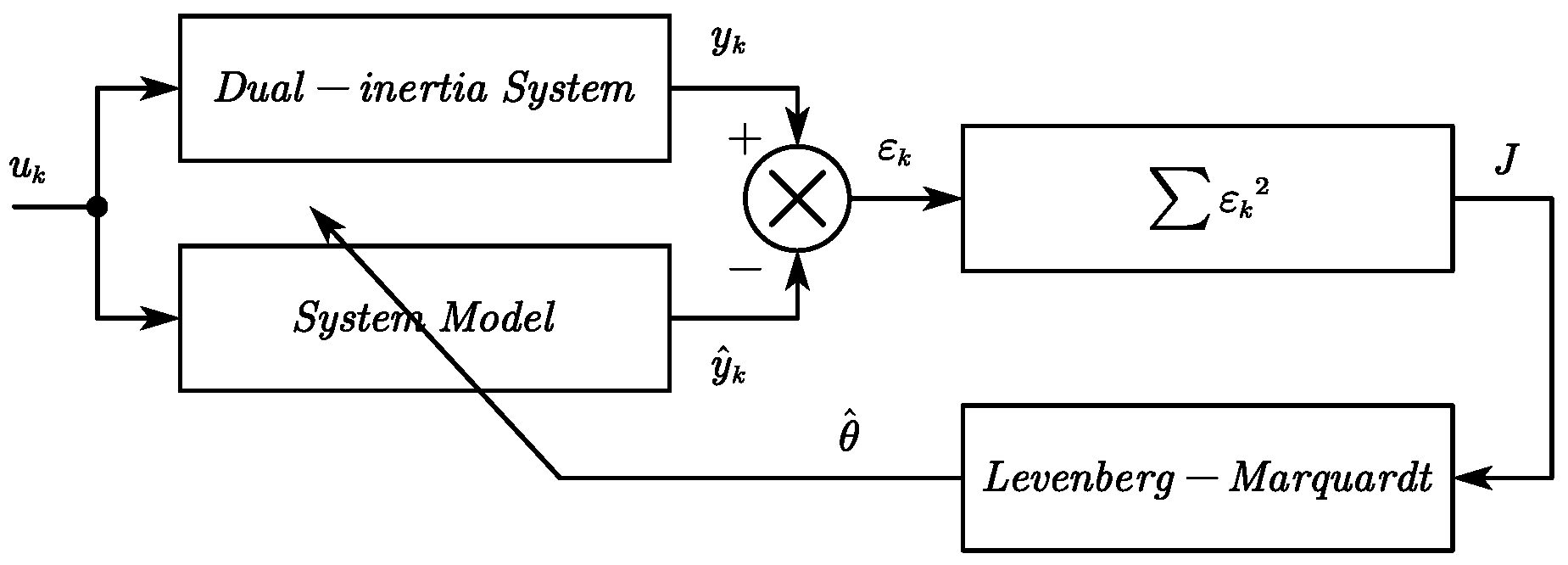
- A model identification approach for the dual-inertia servo system in the time domain was developed, ensuring the effectiveness of the fractional-order dual-inertia servo model.
- (3)
- Experiments involving the dual-inertia servo model and the identification algorithm were carried out on the test platform. The proposed method and model were evaluated against the existing integer-order model. It was verified that the proposed fractional-order servo model has higher accuracy than the integer-order one.
2. The Fractional-Order Modeling of Dual-Inertia Servo Inverter Systems
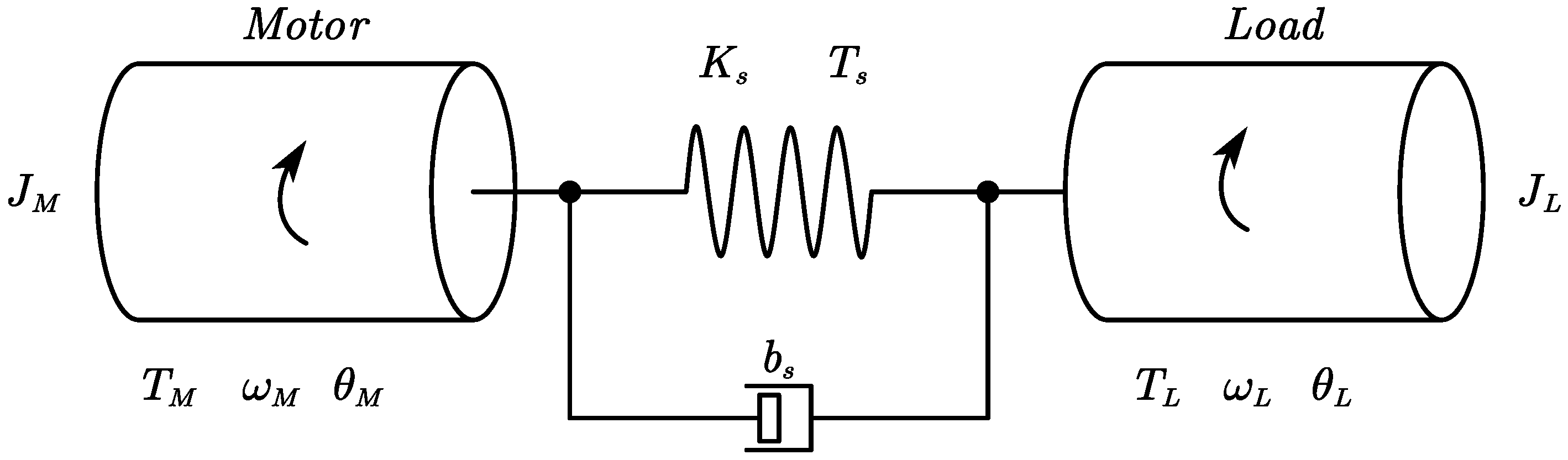
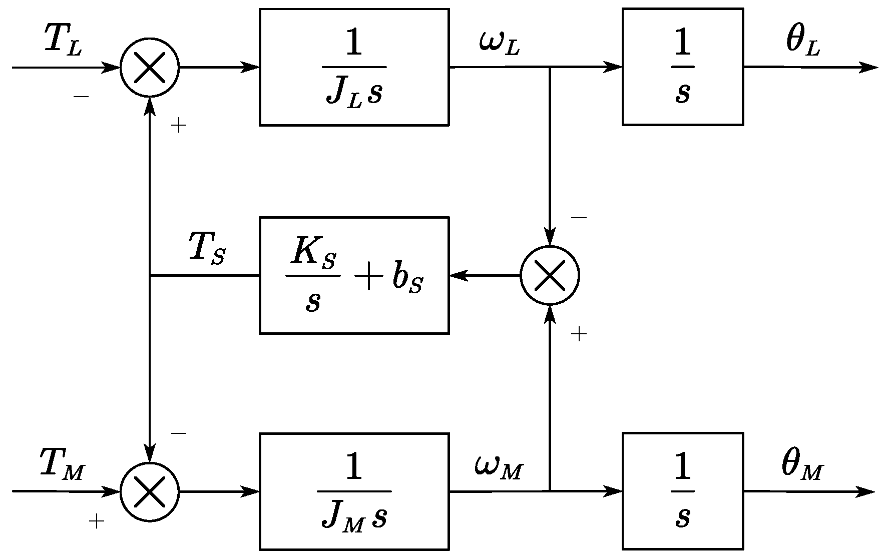
2.1. Integer-Order Dual-Inertia Servo System Model
2.2. Fractional-Order Dual-Inertia Servo System Model
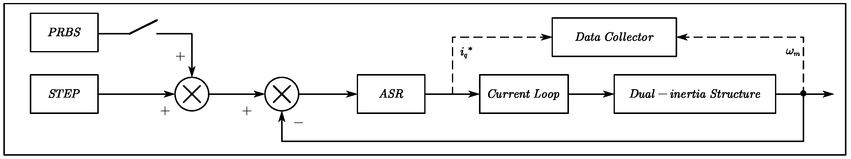
3. Identification for Dual-Inertia Servo Inverter Systems
4. Experimental Demonstration
4.1. Experimental Setup
4.2. Experimental Data Collection
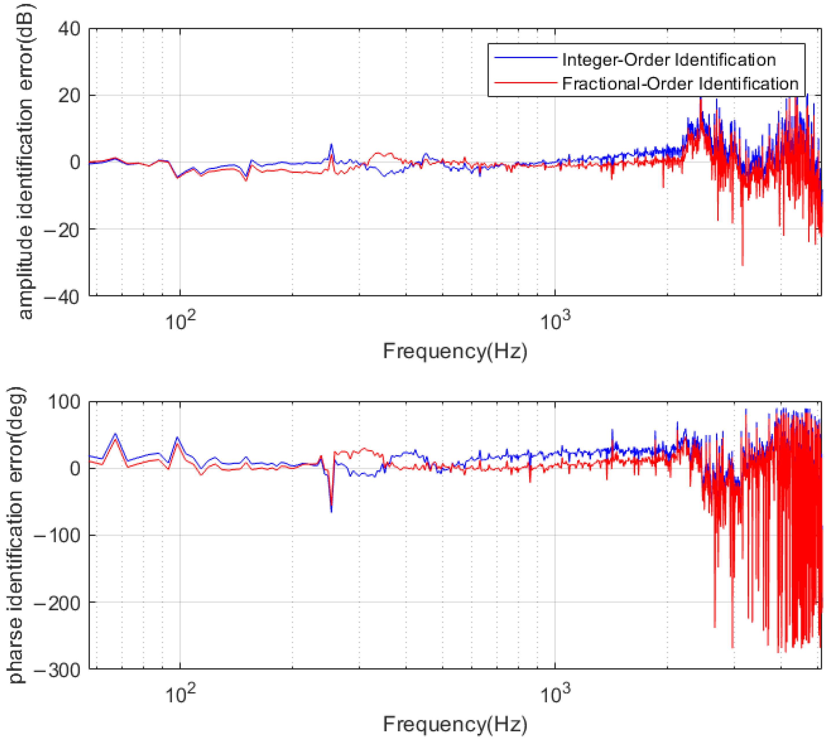
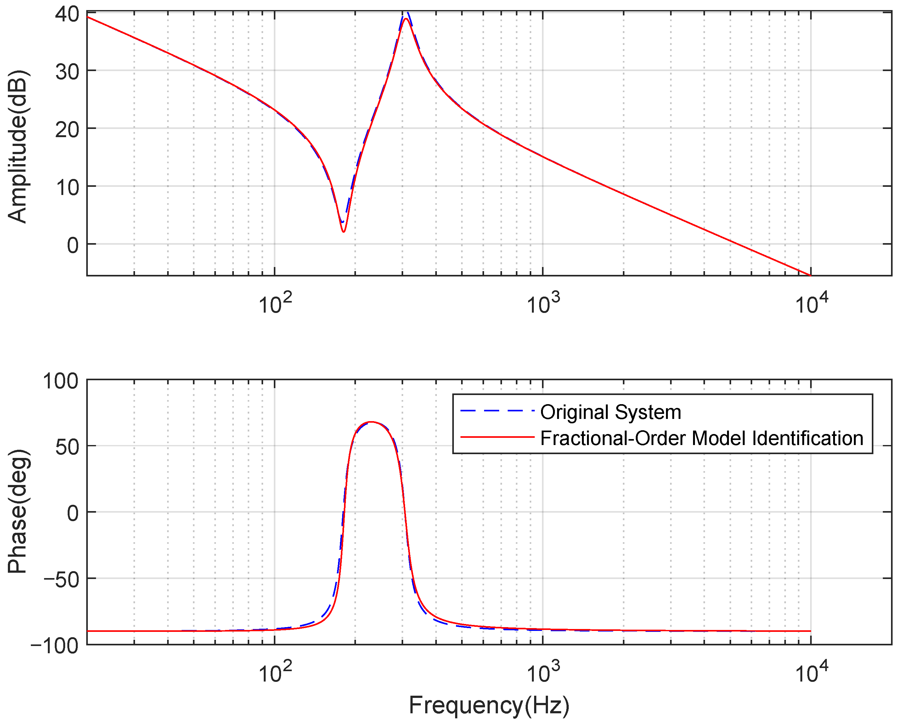
4.3. Parameter Identification
4.4. Noise Sensitivity Test
- (1)
- (2)
- (3)
5. Conclusions
Author Contributions
Funding
Data Availability Statement
Conflicts of Interest
References
- Chen, P.; Luo, Y. Analytical Fractional-Order PID Controller Design With Bode’s Ideal Cutoff Filter for PMSM Speed Servo System. IEEE Trans. Ind. Electron. 2023, 70, 1783–1793. [Google Scholar] [CrossRef]
- Li, P.; Wang, L.; Zhong, B.; Zhang, M. Linear Active Disturbance Rejection Control for Two-Mass Systems Via Singular Perturbation Approach. IEEE Trans. Ind. Inform. 2022, 18, 3022–3032. [Google Scholar] [CrossRef]
- Ming, Y.; Hao, H.; Dian-guo, X. Cause and suppression of mechanical resonance in PMSM servo system. Electr. Mach. Control 2012, 16, 79–84. [Google Scholar]
- Niu, Z.; Huang, W.; Zhu, S. Online Identification of Mechanical Systems Using the Simplified Output Error Model. IEEE Trans. Ind. Electron. 2023, 70, 6653–6662. [Google Scholar] [CrossRef]
- Xu, F. Research on Mechanical Resonance Suppression Algorithm of Permanent Magnet AC servo System. Master’s Thesis, South China University of Technology, Guangzhou, China, 2023. [Google Scholar]
- Xia, J.; Guo, Z.; Li, Z. Optimal Online Resonance Suppression in a Drive System Based on a Multifrequency Fast Search Algorithm. IEEE Access 2021, 9, 55373–55387. [Google Scholar] [CrossRef]
- Yokoyama, M.; Petrea, R.A.B.; Oboe, R.; Shimono, T. External Force Estimation in Linear Series Elastic Actuator Without Load-Side Encoder. IEEE Trans. Ind. Electron. 2021, 68, 861–870. [Google Scholar] [CrossRef]
- Chen, Y.; Yang, M.; Long, J.; Hu, K.; Xu, D.; Blaabjerg, F. Analysis of Oscillation Frequency Deviation in Elastic Coupling Digital Drive System and Robust Notch Filter Strategy. IEEE Trans. Ind. Electron. 2019, 66, 90–101. [Google Scholar] [CrossRef]
- Wang, C.; Yang, M.; Luan, T.; Xu, D. A Review of External Mechanical Parameter Identification of Two-mass Elastic Servo Systems. Proc. Csee 2016, 36, 804–817. [Google Scholar] [CrossRef]
- Zheng, l.; Wu, Y.; Wang, X.; Huang, Q. A Closed-loop Identification Method for Elastic Load of Servo System. Control Theory Appl. 2023, 40, 468–476. [Google Scholar]
- Wen, C.; Tan, M.; Lu, J.; Su, W. Identification of electromechanical servo systems with flexible characteristics. Control Theory Appl. 2023, 40, 663–672. [Google Scholar]
- Villwock, S.; Pacas, M. Application of the Welch-method for the identification of two- and three-mass-systems. IEEE Trans. Ind. Electron. 2008, 55, 457–466. [Google Scholar] [CrossRef]
- Kim, S. Moment of Inertia and Friction Torque Coefficient Identification in a Servo Drive System. IEEE Trans. Ind. Electron. 2019, 66, 60–70. [Google Scholar] [CrossRef]
- Yu, Z.; Tang, T. Bounded-saturation-based disturbance observer for precision position control of an indirect transmission system. Nonlinear Dyn. 2024, 112, 4507–4527. [Google Scholar] [CrossRef]
- Pan, Z.; Wang, X.; Zheng, Z.; Tian, L. Fractional-Order Linear Active Disturbance Rejection Control Strategy for Grid-Side Current of PWM Rectifiers. IEEE J. Emerg. Sel. Top. Power Electron. 2023, 11, 3827–3838. [Google Scholar] [CrossRef]
- Naseri, F.; Karimi, S.; Farjah, E.; Schaltz, E. Supercapacitor management system: A comprehensive review of modeling, estimation, balancing, and protection techniques. Renew. Sustain. Energy Rev. 2022, 155, 111913. [Google Scholar] [CrossRef]
- Mawonou, K.S.R.; Eddahech, A.; Dumur, D.; Beauvois, D.; Godoy, E. Improved state of charge estimation for Li-ion batteries using fractional order extended Kalman filter. J. Power Sources 2019, 435, 226710. [Google Scholar] [CrossRef]
- Bingi, K.; Prusty, B.R.; Singh, A.P. A Review on Fractional-Order Modelling and Control of Robotic Manipulators. Fractal Fract. 2023, 7, 77. [Google Scholar] [CrossRef]
- Baba, I.A.; Humphries, U.W.; Rihan, F.A.A. Role of Vaccines in Controlling the Spread of COVID-19: A Fractional-Order Model. Vaccines 2023, 11, 145. [Google Scholar] [CrossRef]
- Qiao, Y.; Ding, Y.; Pang, D.; Wang, B.; Lu, T. Fractional-Order Modeling of COVID-19 Transmission Dynamics: A Study on Vaccine Immunization Failure. Mathematics 2024, 12, 3378. [Google Scholar] [CrossRef]
- Ai, W.; Lin, X.; Luo, Y.; Wang, X. Fractional-Order Modeling and Identification for an SCR Denitrification Process. Fractal Fract. 2024, 8, 524. [Google Scholar] [CrossRef]
- Zheng, W.; Luo, Y.; Chen, Y.; Pi, Y. Fractional-order modeling of permanent magnet synchronous motor speed servo system. J. Vib. Control 2016, 22, 2255–2280. [Google Scholar] [CrossRef]
- Oustaloup, A.; Levron, F.; Mathieu, B.; Nanot, F. Frequency-band complex noninteger differentiator: Characterization and synthesis. IEEE Trans. Circuits Syst.-Fundam. Theory Appl. 2000, 47, 25–39. [Google Scholar] [CrossRef]
- Hilfer, R. (Ed.) Application of Fractional Calculus in Physics; World Scienctific: Singapore, 2000. [Google Scholar]
- Ferdi, Y. Impulse invariance-based method for the computation of fractional integral of order. Comput. Electr. Eng. 2009, 35, 722–729. [Google Scholar] [CrossRef]
- Podlubny, I.; Petrás, I.; Vinagre, B.; O’Leary, P.; Dorcák, L. Analogue realizations of fractional-order controllers. Nonlinear Dyn. 2002, 29, 281–296. [Google Scholar] [CrossRef]
- Matsuda, K.; Fujii, H. Hoptimized wave-absorbing control: Analytical and experimental results. J. Guid. Control. Dyn. 1993, 16, 1146–1153. [Google Scholar] [CrossRef]
- Xue, D. Fractional Calculus and Fractional-Order Control; Science Press: Beijing, China, 2018. [Google Scholar]
- Madsen, K.; Nielsen, H.; Tingleff, O. Methods for Non-Linear Least Squares Problems; Informatics and Mathematical Modelling Technical University of Denmark: Kongens Lyngby, Denmark, 2004. [Google Scholar]
- Yuan, Y.; Chen, B. Control Systems of Electric Drives-Motion Control System; China Machine Press: Beijing, China, 2009. [Google Scholar]
- Saarakkala, S.E.; Hinkkanen, M. Identification of Two-Mass Mechanical Systems in Closed-Loop Speed Control. In Proceedings of the 39th Annual Conference of the IEEE Industrial-Electronics-Society (IECON), Vienna, Austria, 10–14 November 2013; pp. 2905–2910. [Google Scholar]
- Li, B. Pseudorandom Signal and Correlation Identification; Science Press: Beijing, China, 1987. [Google Scholar]


| Parameter | Nominal Value |
|---|---|
| Speed loop bandwidth | 30 Hz |
| Current loop bandwidth | 2000 Hz |
| Motor power of drive motor | 400 W |
| Motor power of load motor | 400 W |
| Nominal speed of drive motor | 3000 r/min |
| Nominal speed of load motor | 3000 r/min |
| Nominal torque of drive motor | 1.27 N·m |
| Nominal torque of load motor | 1.27 N·m |
| Inertia of drive motor | 6.80 × 10⁻⁵ kg·m2 |
| Inertia of load motor | 6.80 × 10⁻⁵ kg·m2 |
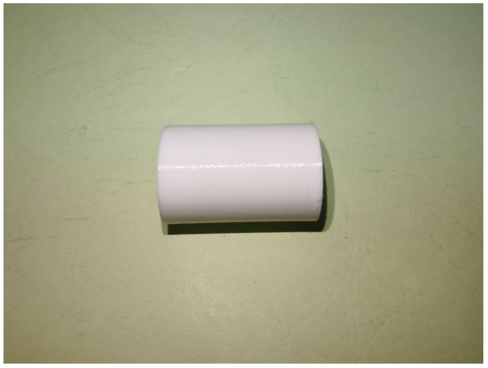
| Diameter of the coupling | 20 mm |
| Length of the coupling | 30 mm |
| Data sampling frequency | 16 kHz |
| Parameter | Integer-Order Model | Fractional-Order Model |
|---|---|---|
| 1 | 0.955 | |
| 1 | 1.382 | |
| 1 | 1.057 | |
| (kg·m2) | ||
| (kg·m2) | ||
| (N/rad) | 224 | 225 |
| (N/rad/s) | 0.0113 | 0.0555 |
| (N/rad/s) | 0.0084 | 0.0098 |
| Integer-Order Identification | Fractional-Order Identification | |
|---|---|---|
| Sum of squared amplitude errors (dB2) | ||
| Sum of squared phase errors (deg2) |
| Integer-Order Identification | Fractional-Order Identification | |
|---|---|---|
| Sum of squared speed errors (RPM2) |
Disclaimer/Publisher’s Note: The statements, opinions and data contained in all publications are solely those of the individual author(s) and contributor(s) and not of MDPI and/or the editor(s). MDPI and/or the editor(s) disclaim responsibility for any injury to people or property resulting from any ideas, methods, instructions or products referred to in the content. |
© 2025 by the authors. Licensee MDPI, Basel, Switzerland. This article is an open access article distributed under the terms and conditions of the Creative Commons Attribution (CC BY) license (https://creativecommons.org/licenses/by/4.0/).
Share and Cite
Wang, X.; Su, Y.; Luo, Y.; Liang, T.; Hu, H. Fractional-Order Modeling and Identification for Dual-Inertia Servo Inverter Systems with Lightweight Flexible Shaft or Coupling. Fractal Fract. 2025, 9, 222. https://doi.org/10.3390/fractalfract9040222
Wang X, Su Y, Luo Y, Liang T, Hu H. Fractional-Order Modeling and Identification for Dual-Inertia Servo Inverter Systems with Lightweight Flexible Shaft or Coupling. Fractal and Fractional. 2025; 9(4):222. https://doi.org/10.3390/fractalfract9040222
Chicago/Turabian StyleWang, Xiaohong, Yijian Su, Ying Luo, Tiancai Liang, and Hengrui Hu. 2025. "Fractional-Order Modeling and Identification for Dual-Inertia Servo Inverter Systems with Lightweight Flexible Shaft or Coupling" Fractal and Fractional 9, no. 4: 222. https://doi.org/10.3390/fractalfract9040222
APA StyleWang, X., Su, Y., Luo, Y., Liang, T., & Hu, H. (2025). Fractional-Order Modeling and Identification for Dual-Inertia Servo Inverter Systems with Lightweight Flexible Shaft or Coupling. Fractal and Fractional, 9(4), 222. https://doi.org/10.3390/fractalfract9040222