Article

On the Pseudospectral Method for Solving the Fractional Klein–Gordon Equation Using Legendre Cardinal Functions

1
School of Mathematics and Statistics, Northeastern University at Qinhuangdao, Qinhuangdao 066004, China
2
Sydney Smart Technology College, Northeastern University at Qinhuangdao, Qinhuangdao 066004, China
3
Department of Mathematics, Institute for Advanced Studies in Basic Sciences (IASBS), Zanjan 45137-66731, Iran
4
Scientific Research Center, Baku Engineering University, Baku AZ0102, Azerbaijan
5
Department of Scientific Research, Innovation and Training of Scientific and Pedagogical Staff, University of Economics and Pedagogy, Karshi 180100, Uzbekistan
6
Department of Electronics and Communication Engineering, Faculty of Engineering, Mansoura University, Mansoura 35516, El-Dakahilia, Egypt
*
Author to whom correspondence should be addressed.
Fractal Fract. 2025, 9(3), 177; https://doi.org/10.3390/fractalfract9030177
Submission received: 23 January 2025 / Revised: 6 March 2025 / Accepted: 12 March 2025 / Published: 14 March 2025

Abstract

This work introduces the Legendre cardinal functions for the first time. Based on Jacobi and Lobatto grids, two approaches are employed to determine these basis functions. These functions are then utilized within the pseudospectral method to solve the fractional Klein–Gordon equation (FKGE). Two numerical schemes based on the pseudospectral method are considered. The first scheme reformulates the given equation into a corresponding integral equation and solves it. The second scheme directly addresses the problem by utilizing the matrix representation of the Caputo fractional derivative operator. We provide a convergence analysis and present numerical experiments to demonstrate the convergence of the schemes. The convergence analysis shows that convergence depends on the smoothness of the unknown function. Notable features of the proposed approaches include a reduction in computations due to the cardinality property of the basis functions, matrices representing fractional derivative and integral operators, and the ease of implementation.

1. Introduction

Fractional calculus and fractional differential equations (FDEs) have emerged as powerful mathematical tools with a profound impact on almost all fields of science and engineering. While classical calculus deals with integer-order derivatives and integrals, fractional calculus generalizes these operators to non-integer orders. As a result, systems with memory and hereditary properties can be modeled using fractional calculus. This capability is particularly valuable for describing entire classes of phenomena that exhibit anomalous diffusion, viscoelastic behavior, and long-range dependencies—features that often cannot be captured by traditional models. FDEs arise in a wide range of applications, including fluid dynamics, control theory, signal processing, and biological systems, where they provide a more realistic modeling of real processes compared to their classical counterparts. Fractional calculus is an important area of modern mathematics because it helps us understand complex systems and solve challenging problems.
Analytical and numerical methods are required to solve FDEs. Analytical methods include the Laplace transform, the Fourier transform, and expansions involving Mittag–Leffler functions, which provide exact solutions for certain classes of FDEs. However, it is commonly known these methods are usually limited to linear or simple nonlinear problems and are insufficient for handling more complicated or higher-dimensional fractional partial differential equations (FPDEs). If such methods exist to solve complicated problems, the literature is quite limited due to the associated difficulties. As a result, numerical methods have become essential tools for addressing FDEs. Numerical approximations for FPDEs, particularly for problems that are difficult to solve analytically, often rely on techniques such as the finite difference method [1], the spectral element method [2,3], the finite element method [4], nonuniform difference schemes [5], the Galerkin method [6,7], the collocation method [8,9], the fractional differential transform method [10], and the kernel-based pseudo-spectral method [11]. For further study, we refer readers to [12,13]. Such numerical approaches enable researchers to tackle real-world problems involving irregular domains, complex boundary conditions, and nonlinearities.
Given Ω = [ a , b ] × [ 0 , τ ] , the fractional Klein–Gordon equation (FKGE) we consider in this paper reads
D t κ a C y ( x , t ) + d 1 2 x 2 y ( x , t ) + d 2 F ( x , t , y ( x , t ) ) = g ( x , t ) , ( x , t ) Ω , κ ( 1 , 2 ] ,
subjected to conditions
y ( x , 0 ) = ϕ 2 ( x ) , D t ( y ( x , t ) ) | t = 0 = ϕ 3 ( x ) , x [ a , b ] ,
y ( a , t ) = ϕ 0 ( t ) , y ( b , t ) = ϕ 1 ( t ) , t [ 0 , τ ] ,
where d 1 and d 2 are constants, the functions g, F are sufficiently smooth functions, and ϕ i for i = 0 , 3 are known. Furthermore, the function F satisfies the Lipschitz condition
| F ( x , t , y 1 ( x , t ) ) F ( x , t , y 2 ( x , t ) ) | L | y 1 ( x , t ) y 2 ( x , t ) | ,
with Lipschitz constant L. The derivative operators D t κ a C and D t refer to Caputo fractional derivative (CFD) and derivative with respect to variable t, respectively.
As we know, both linear and nonlinear Klein–Gordon equations play an important role in modeling various physical phenomena within a wide scope of applications: solitons, condensed matter physics, and classical and quantum mechanics [14] are only a few among others. Originally, the equation was proposed in 1926 by physicists Oskar Klein [15] and Walter Gordon [16] to model relativistic electrons. Given the importance of such equations, the study and determination of their solutions are quite significant [17]. Recently, much attention has been given to the FKGE. Essentially, it serves as a generalization of the integer-order Klein–Gordon equation and further extends the range of applicability. This equation also models non-locality in space and time with the help of power-law kernels [3]. Rapid developments have occurred in presented numerical methods for solving the FPDEs, and especially the FKGE, in recent years, including the following: the Sinc–Chebyshev collocation method [18], homotopy perturbation method [19], the third-kind Chebyshev collocation method [20], cubic B-spline method [21], meshless method [22], Fourier transform method [23], finite difference methods [24], and spectral collocation methods [25].
Essentially, the pseudospectral method among the spectral methods relies on the basic minimization of a residual function at some collocation points and is usually very accurate and efficient. Its simplicity and effectiveness arise from the fact that one is making sure the residual is minimized, and if well implemented, the method always outperforms many other numerical techniques. The method takes advantage of orthogonal polynomials or even trigonometric functions for approximations and realizes exponential convergence in problems with smooth solutions. The pseudospectral method is, therefore, seen as the best option in handling differential equations due to better accuracy and efficiency in computation, including those involving nonlinearities and high-dimensional cases [26].
Cardinal functions serve as a set of basis functions in numerical analysis and approximation theory. They play a critical role in constructing interpolants or approximating functions from discrete data points, making them particularly valuable in spectral and pseudospectral techniques. While some cardinal functions exhibit orthogonality, which streamlines computations in functional spaces, they are predominantly employed in spectral and pseudospectral methods as the bases. The significance of these bases can be examined from two perspectives:
  • Accuracy: Cardinal functions enable spectral accuracy in numerical approaches, delivering highly accurate approximations for solutions to differential equations. In scenarios demanding high accuracy, pseudospectral methods demonstrate superior performance compared to finite difference and finite element methods.
  • Computational Efficiency: The inherent sparsity or localized nature of certain cardinal functions reduces the computational cost of interpolation and quadrature, enhancing overall efficiency.
The outline of this paper is as follows. We introduce the Legendre cardinal function and its properties in the next section. In the section, the matrix form of fractional integral derivatives and the CFD is also presented. In Section 3, two numerical schemes based on the pseudospectral method are developed and implemented for solving FKGEs. The convergence analysis is also investigated. Some numerical experiments are implemented, and the results are reported in Section 4. In Section 5, we provide some final observations and conclusions.

2. Legendre Cardinal Functions

Legendre polynomials are specified as the eigenfunctions of the well-known Sturm–Liouville equation
D x ( 1 x 2 ) D x ( y ( x ) ) + λ y ( x ) = 0 ,
corresponding to the eigenvalues λ m = m ( m + 1 ) . Here, D x indicates the derivative operative with respect to the independent variable x. There are some explicit expressions of these polynomials; among them, the following formula can be mentioned:
L m ( x ) = 1 2 m i = 0 m m i 2 ( x + 1 ) i ( x 1 ) m i .
This expression derivates Rodrigues’ formula, obtained under the normalization L m ( 1 ) = 1 . The three-term recurrence formula for these polynomials holds as follows:
L 0 ( x ) = 1 , L 1 ( x ) = x , ( m + 1 ) L m + 1 ( x ) = ( 2 m + 1 ) x L m ( x ) m L m 1 ( x ) , m 1 ,
These polynomials are orthogonal with respect to the L 2 norm on [ 1 , 1 ] , viz.,
( L m ( x ) , L m ( x ) ) 2 = 1 1 L m ( x ) L m ( x ) d x = 2 2 m + 1 δ m , m ,
where ( . , . ) states the inner product of L 2 [ 1 , 1 ] and δ m , m specifies the Kronecker delta.
Note that the shifted Legendre polynomials on the generic interval [ a , b ] can be introduced through the suitable variable change, i.e.,
L m * ( x ) = L m 2 ( x a ) ( b a ) 1 , m = 0 , 1 , , M .
Explicit expressions for the roots of Legendre polynomials do not exist, and thus numerical computation is required to find them. Generally, two effective algorithms are used for this: the eigenvalue method and the iterative procedure. All the roots of Legendre polynomials are simple, real, and lie in the interval [ 1 , 1 ] . Based on the construction of the shifted Legendre polynomials, their roots can be determined using
x m * = a + ( x m + 1 ) ( b a ) 2 , m = 0 , 1 , , M .
Set the nodes { x m * } m = 0 M as the shifted Legendre polynomial roots; the Legendre cardinal functions associated with these nodes are determined as
c m ( x ) L M + 1 * ( x ) D x ( L M + 1 * ( x m * ) ) ( x x m * ) , m = 0 , 1 , , M , x [ a , b ] ,
Another way to determine the Legendre cardinal functions is to take a grid specified by the extrema of the Legendre polynomial L M * ( x ) and add the endpoints, namely,
{ x m * } m = 0 M = { x ^ m * } m = 0 M 2 { a , b } | D x ( L M * ( x ) ) | { x ^ m * } m = 0 M = 0 .
This set of nodes is often called the Lobatto grid. Associated with this grid, called the Lobatto grid, the Legendre cardinal functions are defined as follows:
c m ( x ) ( 1 x 2 ) D x ( L M * ( x ) ) D x ( 1 x m * 2 ) D x ( L M * ( x m * ) ) ( x x m * ) , m = 0 , 1 , , M x [ a , b ] .
The main characteristic of Legendre cardinal functions is
c m ( x m ¯ * ) = δ m , m ¯ , m , m ¯ = 0 , 1 , , M .
This property allows an M-degree polynomial to interpolate exactly M + 1 data points of the function y. Strictly speaking, any function with M + 1 data points is approximated by
y ( x ) Q M ( y ( x ) ) = m = 0 M y ( x m * ) c m ( x ) .
where Q M : L 2 [ a , b ] Π M [ a , b ] is a projection operator and Π M [ a , b ] indicates the space of polynomials of degree less than M. This approximation is computationally significant because it avoids the integration when calculating expansion coefficients.
Given a two-dimensional function y ( x , t ) L 2 ( Ω ) with Ω = [ a , b ] × [ 0 , τ ] , one can approximate it as follows:
y ( x , t ) Q M ( y ( x , t ) ) = m = 0 M m = 0 M y m , m c m ( x ) c m ( t ) Π M 2 ( Ω ) ,
in which y m , m = y ( x m * , t m * ) and Π M 2 ( Ω ) states the space of the quadratic polynomial on Ω .
Given w α , β ( x ) = ( 1 x ) α ( 1 + x ) β for α , β > 1 , let w ^ α , β ( x ) = w α , β 2 ( x a ) ( b a ) 1 , w ^ α , β ( t ) = w α , β 2 t η 1 and w ^ α , β ( x , t ) = w ^ α 1 , β 1 ( x ) × w ^ α 2 , β 2 ( t ) . Furthermore, assume that
ϝ i = n N 0 2 : 2 n i n ; n j { 0 , 1 } , j i ; i = 1 2 n i = n , 1 i 2 .
We consider the space B α , β n ( Ω ) for n 2 as defined in [27], with the norm and semi-norm
| y | B α , β n ( Ω ) 2 = i = 1 2 n ϝ i D x n ( y ) w ^ α + n i e i , β + n i e i 2 , y B α , β n ( Ω ) 2 = y w ^ α , β 2 + | y | B α , β n ( Ω ) 2 ,
where x = ( x , t ) , α = ( α 1 , α 2 ) , β = ( β 1 , β 2 ) , and e i for i = 1 , 2 indicates the standard-basis vectors. Throughout the paper, we denote C as a positive constant, which can differ in various formulas.
Theorem 1
(cf. Theorem 8.6, [27]). Let 0 indicates the zero vector. Given α , β = 0 , assume that y B 0 , 0 n ( Ω ) . If 2 n M + 1 , then
Q M ( y ) y L 2 ( Ω ) C ( M + 1 n ) ! M ! ( M + n ) ( n + 1 ) / 2 h max 2 2 n | y | B 0 , 0 n ( Ω ) ,
where h max = max { ( b a ) , τ } .

2.1. Derivative Operator in the Matrix Form

This section presents a framework to show how the derivative operator acting on Legendre cardinal functions can be represented as a matrix. Recall that (see, e.g., [27]) the leading coefficients of Legendre polynomials L M + 1 * ( x ) are given as
η M = Γ ( 2 M + 1 ) ( b a ) M Γ ( M + 1 ) 2 ,
and taking the derivative of it leads to
D x k ( L M + 1 * ) ( x ) = ρ M + 1 , k L M + 1 k * ( x ) ,
where the constant ρ M + 1 , k is equal to
ρ M + 1 , k = Γ ( M + k ) 2 k 1 ( b a ) Γ ( M ) .
Taking into account Equations (15) and (17), an alternative representation of the Legendre cardinal functions (8) and (9) is available as follows:
c m ( x ) = σ i = 0 , i m M ( x x i * ) , m = 0 , 1 , , M , x [ a , b ] ,
where σ is equal to η M D x ( L M + 1 * ( x ) ) | x = x m * and 4 ρ M + 1 , 1 Γ ( 2 M 1 ) ( M 2 ) ( b a ) M Γ ( M + 1 ) D x ( 1 x 2 ) D x ( L M * ( x ) ) | x = x m * for (8) and (9), respectively.
Taking the derivative on both sides of (18) leads to
D x ( c m ) ( x ) = σ l = 0 l m M i = 0 i m , l M ( x x i * ) = l = 0 l m M c m ( x ) ( x x l * ) , m = 0 , 1 , , M .
If D x ( c m ( x ) ) is estimated based on the Legendre cardinal functions c m ( x ) , it is easy to verify that
D x ( c m ( x ) ) m = 0 M D x ( c m ( x ) ) | x = x m * c m ( x ) , m = 0 , 1 , , M .
Thus, it results from (19) and (20) that
D x ( c m ( x ) ) | x m * = l = 0 l m M ( x m * x l * ) 1 , m = m , σ i = 0 i m , m M ( x m * x i * ) , m m , m = 0 , 1 , , M .
Assume that Ψ M ( x ) is a vector function whose elements are specified by
Ψ M m + 1 ( x ) = c m ( x ) , m = 0 , 1 , , M .
Using this vector function, the matrix form of derivative operator can be determined as
D x ( Ψ M ( x ) ) D Ψ M ( x ) ,
in which the entries of D R ( M + 1 ) × ( M + 1 ) are determined by (21).

2.2. Fractional Integral Operator in Matrix Form

Firstly, a reformulation of Legendre cardinal functions is required to specify the matrix form of the fractional integral operator (FIO) [28,29], viz.,
i = 0 i m M ( x x i * ) = j = 0 M ϱ m , j x M j ,
in which
ϱ m , 0 = 1 , ϱ m , j = 1 j k = 0 j u m , k ϱ m , j k , u m , k = l = 0 l m M ( x l * ) k m , j = 0 , 1 , M .
Thus, an alternative formula of the Legendre cardinal functions can be determined as follows:
c m ( x ) = σ j = 0 M ϱ m , j x M j , m = 0 , 1 , , M , x [ a , b ] .
Given the value of “a” (the left endpoint of the generic interval [ a , b ] ), two cases must be considered:
If a = 0 : Considering the definition of FIO and gamma function [30], one can prove that
I a κ ( x ) ϑ = Γ ( ϑ + 1 ) Γ ( ϑ + κ + 1 ) x κ + ϑ , κ R + , x [ a , b ] .
Given (26) and considering the reformulation (25), one obtains the result of acting FIO on the Legendre cardinal function, i.e.,
I a κ ( c m ( x ) ) = σ I a κ ( j = 0 M ϱ m , j x M j ) = σ j = 0 M ϱ m , j Γ ( M j + 1 ) Γ ( M j + κ + 1 ) x M j + κ , m = 0 , 1 , , M .
If a 0 , it results that
I a κ ( x ) ϑ = 1 Γ ( κ ) a t ( x ξ ) κ 1 ξ ϑ d ξ = ( x a ) κ a ϑ Γ ( κ ) 0 1 ( 1 t ) κ 1 1 t ( 1 x a ) ϑ d x ( ξ = a + t ( x a ) ) = ( x a ) κ a ϑ Γ ( κ ) B ( 1 , κ ) 2 F 1 ( ϑ , 1 ; κ + 1 ; 1 x a ) ,
(see e.g., ([31]), p.65),
where B and 2 F 1 state the beta and hypergeometric functions [31], respectively. Thus, it proves from (25) and (28) that
I a κ ( c m ( x ) ) = σ ( x a ) κ B ( 1 , κ ) Γ ( κ ) j = 0 M ϱ m , j a M j 2 F 1 ( ( M j ) , 1 ; κ + 1 ; 1 x a ) , m = 0 , M .
Now, everything is ready to present the matrix form of FIO based on Legendre cardinal functions, viz.,
I a κ ( c m ( x ) ) m = 0 M I a κ ( c m ) ( x m * ) c m ( x ) , m = 0 , M ,
where the coefficients I a κ ( c m ) ( x m * ) are calculated through (27) and (29). So, one can introduce a matrix I ϑ R ( M + 1 ) × ( M + 1 ) that satisfies
I a κ ( Ψ M ( x ) ) I κ Ψ M ( x ) ,
and has elements
I κ m + 1 , m + 1 = I a κ ( c m ) ( x m * ) , m , m = 0 , M .

2.3. Caputo Fractional Derivative Operator in Matrix Form

Assume that κ R + and ν = κ (where . is the ceiling function). The CFD operator D x k a C is represented by I a ν κ D ν when κ N 0 . We aim to find a matrix D κ R ( M + 1 ) × ( M + 1 ) that satisfies
D x k a C ( Ψ M ( x ) ) D κ Ψ M ( x ) .
Replacing I a ν κ D ν instead of D x k a C leads to
D x k a C ( Ψ M ( x ) ) = I a ν κ D ν ( Ψ M ( x ) ) D ν I ν κ Ψ M ( x ) .
Thus, without direct calculations, the matrix form of the CFD operator is obtained, viz.,
D κ : = D ν I ν κ .

3. Pseudospectral Method Based on Legendre Cardinal Functions

In the sequel, two numerical schemes based on the pseudospectral method are developed and implemented for solving Equation (1).
First scheme (PS1): A traditional scheme to solve a fractional partial differential equation is to render it into a corresponding integral equation. Our first numerical scheme involves applying the pseudospectral method to solve the integral equation obtained from Equation (1):
y ( x , t ) y 0 ( x , t ) + I a κ d 1 2 x 2 y ( x , t ) + d 2 F ( x , t , y ( x , t ) ) g ( x , t ) = 0 ,
y ( a , t ) = ϕ 0 ( t ) , y ( b , t ) = ϕ 1 ( t ) , t [ 0 , τ ] ,
where y 0 ( x , t ) = y ( x , 0 ) + D t ( y ( x , t ) ) | t = 0 . It is not difficult to prove that the solution to this integral equation is equivalent to the solution of (1) [30]. Let us approximate the unknown y ( x , t ) using the expansion (12) based on Legendre cardinal functions, i.e.,
y ( x , t ) Q M ( y ( x , t ) ) = m = 0 M m = 0 M y m , m c m ( x ) c m ( t ) = Ψ T ( x ) Y Ψ ( t ) Π M 2 ( Ω ) ,
where Y R ( M + 1 ) × ( M + 1 ) whose elements must be found. Substituting the approximate solution y M ( x , t ) : = Q M ( y ( x , t ) ) into (36) instead of y leads to introducing the residual function
r 1 ( x , t ) = y M ( x , t ) y 0 ( x , t ) + I a κ d 1 2 x 2 y M ( x , t ) + d 2 F ( x , t , y M ( x , t ) ) g ( x , t ) .
Thanks to the matrix form of the derivative operator D and FIO I κ in the Legendre cardinal functions, one can write
Q M ( r 1 ( x , t ) ) = Ψ T ( x ) Y Y 0 + d 1 D 2 T Y I κ + d 2 F I κ G I κ Ψ ( t ) ,
in which
y 0 ( x , t ) Q M ( y 0 ( x , t ) ) = Ψ T ( x ) Y 0 Ψ ( t ) , F ( x , t , y M ( x , t ) ) Q M ( F ( x , t , y M ( x , t ) ) ) = Ψ T ( x ) F Ψ ( t ) . g ( x , t ) Q M ( g ( x , t ) ) = Ψ T ( x ) G Ψ ( t ) ,
where Y 0 , F, and G are ( M + 1 ) × ( M + 1 ) matrices.
The objective is to apply the pseudospectral method. Thus, the unknowns can be found by picking the Jacobi or Lobatto grids { x m * } m = 0 M , such that the residual is approximately zero at these points, i.e.,
Q M ( r 1 ( x , t ) ) | ( x , t ) = ( x m * , x m * ) = 0 , m , m = 0 , , M .
Equivalently, we have the nonlinear system
R ( Y ) = Y Y 0 + d 2 D 2 T Y I κ + d 2 F I κ G I κ = 0 .
First, to apply the boundary conditions (37), the functions ϕ 0 ( t ) and ϕ 1 ( t ) must be approximated by Legendre cardinal functions, viz.,
ϕ 0 ( t ) Q M ( ϕ 0 ( t ) ) = Φ 0 T Ψ ( t ) , ϕ 1 ( t ) Q M ( ϕ 1 ( t ) ) = Φ 1 T Ψ ( t ) ,
where Φ i R M + 1 for i = 0 , 1 . By replacing the first and last rows of R ( Y ) with vectors ( ψ T ( a ) Y ) T Φ 0 and ( ψ T ( b ) Y ) T Φ 1 , respectively, a new nonlinear system
R ¯ ( Y ) = 0 ,
is obtained. Solving this system using Newton’s method leads to specifying the unknowns Y.
Second scheme (PS2): The second numerical scheme solves Equation (1) directly without rendering it to an integral equation. Taking into account the approximation (38) and using the matrix form of the CFD operator, one derives
D t κ a C y M ( x , t ) = Ψ T ( x ) Y D κ Ψ ( t ) .
Furthermore, we have
2 x 2 y M ( x , t ) = Ψ T ( x ) D 2 T Y Ψ ( t ) .
Substituting (41), (46), and (47) into (1) enables us to introduce the residual as follows:
r 2 ( x , t ) = Ψ T ( x ) Y D κ + d 1 D 2 T Y + d 2 F G Ψ ( t )
Using collocation points ( x m * , x m * ) for m , m = 0 , , M is sufficient to apply the pseudospectral method, viz.,
R ( Y ) = Y D κ + d 1 D 2 T Y + d 2 F G .
It is necessary to approximate the initial conditions to apply the initial and boundary conditions (2) and (3), in addition to the approximations (44). For this purpose, we have the following:
ϕ 2 ( x ) Q M ( ϕ 2 ( x ) ) = Φ 2 T Ψ ( x ) , ϕ 3 ( x ) Q M ( ϕ 3 ( x ) ) = Φ 3 T Ψ ( x ) ,
where Φ i R M + 1 for i = 2 , 3 . By replacing the first and last rows and columns of R ( Y ) with vectors Φ 0 , Φ 1 , Φ 2 , and Φ 3 , respectively, a new nonlinear system
R ¯ ( Y ) = 0 .
Newton’s method is applied to solve this nonlinear system.

Convergence Analysis

Theorem 2.
Let y be the exact solution of (36) and y M the approximate solution obtained from PS1. If y , g , F B 0 , 0 n ( Ω ) , 2 < n M + 1 , and F satisfies the Lipschitz condition (4), then it can be obtained that
e M L 2 ( Ω ) 0 , a s M ,
where e M = y y M .
Proof. 
Subtracting (36) from (42) leads to
y y M y 0 Q M ( y 0 ) + I a κ d 1 2 x 2 y ( x , t ) + d 2 F ( x , t , y ( x , t ) ) g ( x , t ) Q M I a κ d 1 2 x 2 y M ( x , t ) + d 2 F ( x , t , y M ( x , t ) ) g ( x , t ) = 0 .
Adding and subtracting some terms, we can rewrite this equation as
e M = y 0 Q M ( y 0 ) d 1 I a κ 2 x 2 e M d 2 I a κ F ( x , t , y ) F ( x , t , y M ) + I a κ g Q M ( g ) + d 1 ( I Q M ) I a κ ( 2 x 2 y M ) + d 2 ( I Q M ) I a κ ( F ( x , t , y M ) ) ( I Q M ) I a κ ( Q M ( g ) ) ,
where I is identity operator. Taking the norm from both sides of (52) leads to
e M L 2 ( Ω ) ( I Q M ) ( y 0 ) L 2 ( Ω ) + d 1 I a κ 2 x 2 e M L 2 ( Ω ) + I a κ g Q M ( g ) L 2 ( Ω ) + d 2 I a κ F ( x , t , y ) F ( x , t , y M ) L 2 ( Ω ) + d 1 ( I Q M ) I a κ ( 2 x 2 y M ) L 2 ( Ω ) + d 2 ( I Q M ) I a κ ( F ( x , t , y M ) ) L 2 ( Ω ) + ( I Q M ) I a κ ( Q M ( g ) ) L 2 ( Ω ) .
Taking into account Theorem 1 and using the Lipschitz condition (4) and Lemma 2.1(a) [30], we have
I a κ ( F ( x , t , y ) F ( x , t , y M ) ) L 2 ( Ω ) L I a κ ( e M ) L 2 ( Ω ) L τ Γ ( κ + 1 ) e M L 2 ( Ω ) C L τ Γ ( κ + 1 ) ( M + 1 n ) ! M ! ( M + n ) ( n + 1 ) / 2 h max 2 2 n | y | B 0 , 0 n ( Ω ) .
where h max = max { ( b a ) , τ } . Applying Theorems (3.40) and (8.6) [27] gives rise to writing
I a κ 2 x 2 e M L 2 ( Ω ) τ Γ ( κ + 1 ) 2 x 2 e M L 2 ( Ω ) C τ Γ ( κ + 1 ) ( M + 1 n ) ! M ! ( M + n ) 2 ( n + 1 ) / 2 h max 2 2 n | y | B 0 , 0 n ( Ω ) ,
and
I a κ g Q M ( g ) L 2 ( Ω ) τ Γ ( κ + 1 ) g Q M ( g ) L 2 ( Ω ) C τ Γ ( κ + 1 ) ( M + 1 n ) ! M ! ( M + n ) ( n + 1 ) / 2 h max 2 2 n | g | B 0 , 0 n ( Ω ) .
For the rest of the norms in (53), applying Theorem 1, one can write
( I Q M ) z z M L 2 ( Ω ) C ( M + 1 n ) ! M ! ( M + n ) ( n + 1 ) / 2 h max 2 2 n | z | B 0 , 0 n ( Ω ) ,
where z { y 0 , I a κ ( 2 x 2 y M ) , I a κ ( F ( x , t , y M ) ) , I a κ ( Q M ( g ) ) } .
Considering (54)–(57), it follows from (53) that
e M L 2 ( Ω ) C L τ Γ ( κ + 1 ) ( M + 1 n ) ! M ! ( M + n ) 2 ( n + 1 ) / 2 h max 2 2 n | y | B 0 , 0 n ( Ω ) + C τ Γ ( κ + 1 ) ( M + 1 n ) ! M ! ( M + n ) ( n + 1 ) / 2 h max 2 2 n | u | B 0 , 0 n ( Ω ) ,
in which
| u | B 0 , 0 n ( Ω ) = max | z | B 0 , 0 n ( Ω ) , | g | B 0 , 0 n ( Ω ) .
If y , g , F B 0 , 0 n ( Ω ) and 2 < n M + 1 , then it can be obtained that
e M L 2 ( Ω ) 0 , a s M .
Theorem 3.
Let y be the exact solution of (1) and y M the approximate solution obtained from PS2. If F , g are sufficiently smooth functions, y B 0 , 0 n ( Ω ) , 2 < n M + 1 , and F satisfies the Lipschitz condition (4), then it can be obtained that
e M L 2 ( Ω ) 0 , a s M ,
where e M = y y M .
Proof. 
Subtracting (1) from
Q M ( D t κ a C y M ( x , t ) ) + d 1 Q M ( 2 x 2 y M ( x , t ) ) + d 2 Q M ( F ( x , t , y M ( x , t ) ) ) = Q M ( g ( x , t ) ) ,
leads to
D t κ a C e M + d 1 2 x 2 e M + d 2 F ( x , t , y ) F ( x , t , y M ) + ( I Q M ) ( D t κ a C y M + d 1 2 x 2 y M + d 2 F ( x , t , y M ) g ) = 0 .
For ( x , t ) Ω , using the Cauchy–Schwarz inequality, one can write
e M ( x , t ) = a x s e M ( s , t ) d s a x | s e M ( s , t ) | d s = a x | s e M ( s , t ) . 1 | d s a b | s e M ( s , t ) | 2 d s 1 / 2 . a b 1 d s 1 / 2 = b a a b | s e M ( s , t ) | 2 d s 1 / 2 .
Integrating both sides over Ω after squaring them gives rise to
0 τ a b | e M ( x , t ) | 2 d x d t 0 τ a b ( b a ) a b | s e M ( s , t ) | 2 d s 2 d x d t = ( b a ) 2 0 τ a b | s e M ( s , t ) | 2 d s d t .
Hence,
e M L 2 ( Ω ) ( b a ) x e M L 2 ( Ω ) ( b a ) 2 2 x 2 e M L 2 ( Ω ) .
Given
r ( y M ) = D t κ a C y M + d 1 2 x 2 y M + d 2 F ( x , t , y M ) g .
Consider (59) and (60). Then, using the triangular inequality, we have
1 ( b a ) 2 e M L 2 ( Ω ) | d 1 | 2 x 2 e M L 2 ( Ω ) + | d 2 | F ( x , t , y ) F ( x , t , y M ) L 2 ( Ω ) + D t κ a C e M L 2 ( Ω ) + ( I Q M ) ( r ( y M ) ) L 2 ( Ω )
Taking into account Theorem 1 and using the Lipschitz condition (4), one can obtain
F ( x , t , y ) F ( x , t , y M ) L 2 ( Ω ) C ( M + 1 n ) ! M ! ( M + n ) ( n + 1 ) / 2 h max 2 2 n | y | B 0 , 0 n ( Ω ) .
Recall that D t κ a C : = I a 2 κ D 2 where 1 < κ < 2 . Thus, utilizing Lemma 2.1(a) [30], we have
D t κ a C e M L 2 ( Ω ) I a 2 κ D 2 ( e M ) L 2 ( Ω ) τ Γ ( 3 κ ) D 2 ( e M ) L 2 ( Ω ) .
It follows from using Theorem 1 and Theorems (3.40) and (8.6) [27] that
D t κ a C e M L 2 ( Ω ) C τ Γ ( 3 κ ) ( M + 1 n ) ! M ! ( M + n ) 2 ( n + 1 ) / 2 h max 2 2 n | y | B 0 , 0 n ( Ω ) .
Using Equations (55) and (61)–(63), we have
e M L 2 ( Ω ) C ( M + 1 n ) ! M ! ( M + n ) 2 ( n + 1 ) / 2 h max 2 2 n | y | B 0 , 0 n ( Ω ) + C ( M + 1 n ) ! M ! ( M + n ) ( n + 1 ) / 2 h max 2 2 n | r ( y M ) | B 0 , 0 n ( Ω ) .
If y B 0 , 0 n ( Ω ) and 2 < n M + 1 , then it can be obtained that
e M L 2 ( Ω ) 0 , a s M .

4. Numerical Results

Example 1.
Consider the fractional Klein–Gordon equation
D t κ 0 C y ( x , t ) 2 x 2 y ( x , t ) + s i n ( y ( x , t ) ) = sin ( t 2 sin ( x ) ) + 2 t 2 κ Γ ( 2 κ ) + t 2 sin ( x ) ,
subjected to the following initial and boundary conditions:
y ( x , 0 ) = 0 , D t ( y ( x , t ) ) | t = 0 = 0 , x [ 0 , 1 ] ,
y ( 0 , t ) = 0 , y ( 1 , t ) = t 2 sin ( 1 ) , t [ 0 , 1 ] .
For this example, the exact solution y ( x , t ) = t 2 sin ( x ) is provided in [32].
Table 1 shows the efficiency and accuracy of the two proposed schemes based on Jacobi and Lobatto grids for different values of κ . To compare the proposed methods with existing ones, Table 2 presents comparisons with the implicit RBF meshless method [32]. The results confirm that our schemes yield better outcomes than the implicit RBF meshless method. The L 2 -errors at different times are reported in Table 3 for PS1 with Jacobi grid, Table 4 for PS1 with Lobatto grid, Table 5 for PS2 with Jacobi grid, and Table 6 for PS2 with Lobatto grid. In all tables, the CPU times are also included. 
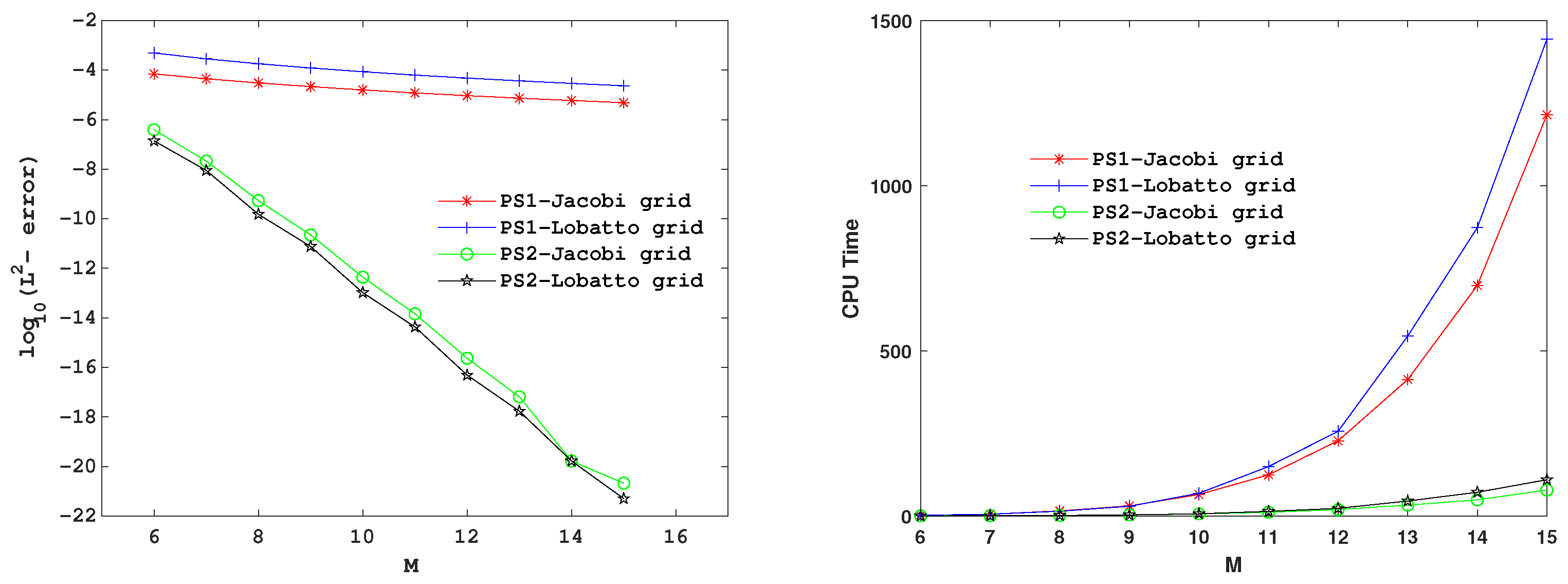
Figure 1 illustrates the convergence of the proposed schemes.
Finally, the accuracy and efficiency of the proposed schemes are validated by the reported results. Additionally, the obtained results support the convergence analysis provided. Moreover, the second scheme yields more accurate results compared to the first scheme. Generally, the best results for this example are achieved by the second scheme using the Lobatto grid (specifically the PS2-Lobatto grid), while requiring less computational time.
Example 2.
Consider the fractional Klein–Gordon equation
D t κ 0 C y ( x , t ) 2 x 2 y ( x , t ) + y ( x , t ) + 3 2 y ( x , t ) 3 = g ( x , t ) ,
subjected to conditions
y ( x , 0 ) = 0 , D t ( y ( x , t ) ) | t = 0 = 0 , x [ 0 , 1 ] ,
y ( 0 , t ) = 0 , y ( 1 , t ) = t 2 + κ sin ( π ) , t [ 0 , 1 ] ,
where g ( x , t ) = sin π x 2 3 sin 2 π x t 6 + 3 κ + Γ 3 + κ t 2 + 2 π 2 t 2 + κ + 2 t 2 + κ .
For this example, the exact solution y ( x , t ) = t 2 + κ sin ( π x ) is reported in [33].
Table 7 displays the accuracy of the two proposed schemes based on Jacobi and Lobatto grids for different values of κ . To compare the proposed methods with existing methods, Table 8 is presented. The variational iteration method [33] and Sinc–Chebyshev collocation method [
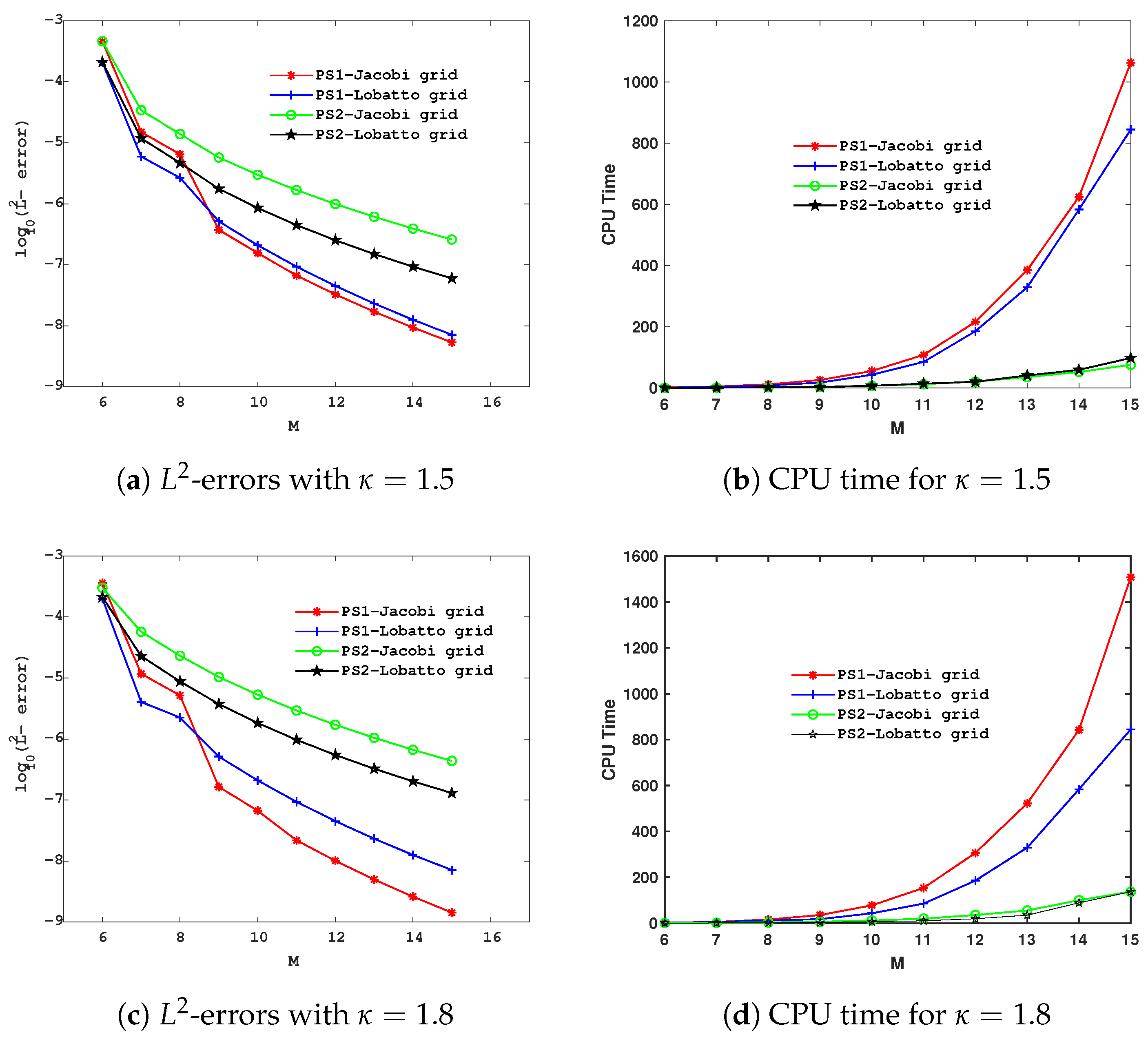
18] are compared with our proposed schemes in this table. The results confirm that our schemes yield better outcomes than these methods. We compared the errors obtained using the different schemes proposed in this paper and plotted them in Figure 2, where CPU times are also reported.
The experimental results indicate that the first scheme is more accurate, while the second scheme executes faster.
Example 3.
Consider the fractional Klein–Gordon equation
D t κ 0 C y ( x , t ) 2 x 2 y ( x , t ) + sin ( y ( x , t ) ) = g ( x , t ) ,
subjected to conditions
y ( x , 0 ) = e x , D t ( y ( x , t ) ) | t = 0 = 0 , x [ 0 , 1 ] ,
y ( 0 , t ) = t 3 + t 2 + 1 , y ( 1 , t ) = e ( t 3 + t 2 + 1 ) , t [ 0 , 1 ] ,
where g ( x , t ) = 6 t 3 κ Γ ( 4 κ ) + 2 t 2 κ Γ ( 3 κ ) ( t 3 + t 2 + 1 ) e x + sin ( ( t 3 + t 2 + 1 ) e x ) .
For this example, the exact solution is y ( x , t ) = ( t 3 + t 2 + 1 ) e x .
Table 9 displays the accuracy of the two proposed schemes based on Jacobi and Lobatto grids for different values of 
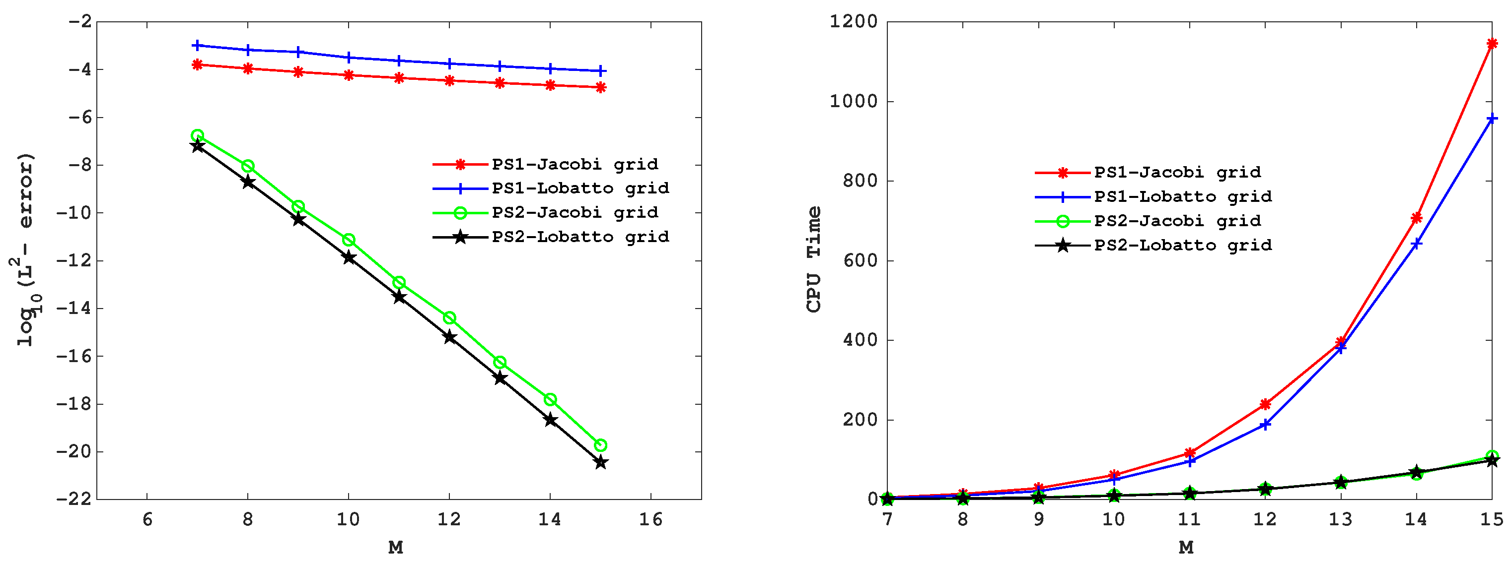
M. We compared the errors obtained using the different schemes proposed in this paper and plotted them in Figure 3, where CPU times are also reported.

5. Conclusions

This paper introduces the Legendre cardinal function for the first time and employs two numerical schemes to solve the fractional Klein–Gordon equation (FKGE). The paper addresses two main subjects: the introduction of the Legendre cardinal functions and the solution of the FKGE. The Legendre cardinal functions are determined using Jacobi and Lobatto grids, both of which satisfy the cardinality condition—a fundamental property of cardinal functions. We represent the fractional integral operator and the Caputo fractional derivative as matrices.
Two numerical schemes based on the pseudospectral method are considered. The first scheme reformulates the given equation into a corresponding integral equation for solving it. The second scheme directly tackles the problem by utilizing the matrix representation of the Caputo fractional derivative operator. The numerical examples validate our convergence analysis. All proposed methods result in accurate solutions. Comparisons with other methods demonstrate that the proposed schemes outperform existing approaches.
Some notable features of the proposed methods include a reduction in computational effort due to the cardinality property of the basis functions, matrices representing fractional derivative and integral operators, and ease of implementation. The presented approaches can be extended to solve higher-dimensional FKGEs. Additionally, these schemes can be used to address other fractional problems, including fractional differential equations, fractional partial differential equations, integral equations with weakly singular kernels, and fractional integro-differential equations.

Author Contributions

Conceptualization, T.L., B.D., B.N.S., D.A.J. and E.E.E.; Methodology, T.L., B.D., B.N.S., D.A.J. and E.E.E.; Software, B.N.S. and D.A.J.; Validation, T.L., B.D., B.N.S., D.A.J. and E.E.E.; Formal analysis, T.L., B.D., B.N.S., D.A.J. and E.E.E.; Investigation, B.N.S. and E.E.E.; Writing—original draft, B.N.S., D.A.J. and E.E.E.; Writing—review & editing, T.L., B.D., B.N.S., D.A.J. and E.E.E.; Visualization, B.N.S., D.A.J. and E.E.E.; Supervision, B.N.S.; Funding acquisition, T.L., B.D. and E.E.E. All authors have read and agreed to the published version of the manuscript.

Funding

This research was funded by the Open Fund Project of the Marine Ecological Restoration and Smart Ocean Engineering Research Center of Hebei Province (HBMESO2321), the Technical Service Project of the Eighth Geological Brigade of the Hebei Bureau of Geology and Mineral Resources Exploration (KJ2022-021), the Technical Service Project of Hebei Baodi Construction Engineering Co., Ltd. (KJ2024-012), the Natural Science Foundation of Hebei Province of China (A2020501007), and the Fundamental Research Funds for the Central Universities (N2123015).

Data Availability Statement

The original contributions presented in this study are included in the article. Further inquiries can be directed to the corresponding author.

Conflicts of Interest

The writers state that they have no known personal relationships or competing financial interests that could have appeared to affect the work reported in this work.

References

  1. Zhang, Y. A finite difference method for fractional partial differential equation. Appl. Math. Comput. 2009, 215, 524–529. [Google Scholar] [CrossRef]
  2. Asadzadeh, M.; Saray, B.N. On a multiwavelet spectral element method for integral equation of a generalized Cauchy problem. BIT 2022, 62, 383–1416. [Google Scholar] [CrossRef]
  3. Liu, T.; Xue, R.; Ding, b.; Juraev, D.; Saray, B.N.; Soleymani, F. A Novel and Effective Scheme for Solving the Fractional Telegraph Problem via the Spectral Element Method. Fractal Fract. 2024, 8, 711. [Google Scholar] [CrossRef]
  4. Ford, N.J.; Xiao, J.; Yan, Y. A finite element method for time fractional partial differential equations. Fract. Calc. Appl. Anal. 2011, 14, 454–474. [Google Scholar] [CrossRef]
  5. Fardi, M.; Zaky, M.A.; Hendy, A.S. Nonuniform difference schemes for multi-term and distributed-order fractional parabolic equations with fractional Laplacian. Math. Comput. Simulat. 2023, 206, 614–635. [Google Scholar] [CrossRef]
  6. Li, C.; Li, Z.; Wang, Z. Mathematical analysis and the local discontinuous Galerkin method for Caputo–Hadamard fractional partial differential equation. J. Sci. Comput. 2020, 85, 41. [Google Scholar] [CrossRef]
  7. Mao, Z.; Shen, J. Efficient spectral–Galerkin methods for fractional partial differential equations with variable coefficients. J. Comput. Phys. 2016, 307, 243–261. [Google Scholar] [CrossRef]
  8. Bonyadi, S.; Mahmoudi, Y.; Lakestani, M.; Jahangiri rad, M. Numerical solution of space-time fractional PDEs with variable coefficients using shifted Jacobi collocation method. Comput. Methods Differ. Equ. 2023, 11, 81–94. [Google Scholar]
  9. Javidi, M. Chebyshev Spectral Collocation Method for Computing Numerical Solution of Telegraph Equation. Comput. Methods Differ. Equ. 2013, 1, 16–29. [Google Scholar]
  10. Günerhan, H.; Çelik, E. Analytical and approximate solutions of fractional partial differential-algebraic equations. Appl. Math. Nonlinear Sci. 2020, 5, 109–120. [Google Scholar] [CrossRef]
  11. Fardi, M. A kernel-based pseudo-spectral method for multi-term and distributed order time-fractional diffusion equations. Numer. Methods Partial. Differ. Equ. 2023, 39, 2630–2651. [Google Scholar] [CrossRef]
  12. Juraev, D.A.; Shokri, A.; Marian, D. Solution of the ill-posed Cauchy problem for systems of elliptic type of the first order. Fractal Fract. 2022, 6, 358. [Google Scholar] [CrossRef]
  13. Juraev, D.A.; Shokri, A.; Marian, D. On the approximate solution of the Cauchy problem in a multidimensional unbounded domain. Fractal Fract. 2022, 6, 403. [Google Scholar] [CrossRef]
  14. Bussey, P.J. Improving our Understanding of the Klein–Gordon Equation. Glob. J. Sci. Front. Res. 2022, 22, 11–19. [Google Scholar]
  15. Klein, O. Quantentheorie und fünfdimensionale Relativitätstheorie. Z. Phys. 1926, 37, 895–906. [Google Scholar] [CrossRef]
  16. Gordon, W. Der Comptoneffekt nach der Schrödingerschen Theorie. Z. Phys. 1926, 40, 117–133. [Google Scholar] [CrossRef]
  17. Aaqib, I.; Rashid, N.; Rashid, A.; Mehran; Fewster-Young, N.; Hina. Extension of optimal auxiliary function method to nonlinear Sine Gordon differential equations. Partial. Differ. Equ. Appl. Math. 2024, 10, 100735. [Google Scholar]
  18. Nagy, A.M. Numerical solution of time fractional nonlinear Klein–Gordon equation using Sinc-Chebyshev collocation method. Appl. Math. Comput. 2017, 310, 139–148. [Google Scholar] [CrossRef]
  19. Golmankhaneh, A.K.; Golmankhaneh, A.K.; Baleanu, D. On nonlinear fractional Klein–Gordon equation. Signal Process 2011, 91, 446–451. [Google Scholar] [CrossRef]
  20. Singh, H.; Kumar, D.; Pandey, R.K. An Efficient Computational Method for the Time-Space Fractional Klein–Gordon Equation. Front Phys. 2020, 8, 281. [Google Scholar] [CrossRef]
  21. Amin, M.; Abbas, M.; Iqbal, M.K.; Baleanu, D. Numerical treatment of time-fractional Klein–Gordon equation using redefined extended cubic B-spline functions. Front Phys. 2020, 8, 288. [Google Scholar] [CrossRef]
  22. Gharian, D.; Ghaini, F.M.M.; Heydari, M.H.; Avazzadeh, Z. A meshless solution for the variable-order time fractional nonlinear Klein–Gordon equation. Int. J. Appl. Comput. Math. 2020, 6, 130. [Google Scholar] [CrossRef]
  23. Mainardi, F. Fractional Calculus and Waves in Linear Viscoelasticity; World Scientific: Singapore, 2010. [Google Scholar]
  24. Chen, S.; Liu, F.; Anh, V. Numerical analysis of the fractional Klein–Gordon equation. J. Comput. Phys. 2007, 227, 941–952. [Google Scholar]
  25. Bhrawy, A.H.; Alghamdi, M.A. A shifted Jacobi-Gauss-Lobatto collocation method for solving nonlinear fractional differential equations. Bound. Value Probl. 2013, 2013, 62. [Google Scholar]
  26. Boyd, J.P. Chebyshev and Fourier Spectral Methods, 2nd ed.; Dover Publications: Garden City, NY, USA, 2001; Revised. [Google Scholar]
  27. Shen, J.; Tang, T.; Wang, L.L. Spectral Methods: Algorithms. Analysis, Applications; Springer: Berlin, Germany, 2011. [Google Scholar]
  28. Sayevand, K.; Arab, H. An efficient extension of the Chebyshev cardinal functions for differential equations with coordinate derivatives of non-integer order. Comput. Methods Differ. Equ. 2018, 6, 339–352. [Google Scholar]
  29. Shahriari, M.; Saray, B.N.; Mohammadalipour, B.; Saeidian, S. Pseudospectral method for solving the fractional one-dimensional Dirac operator using Chebyshev cardinal functions. Phys. Scr. 2023, 98, 055205. [Google Scholar] [CrossRef]
  30. Kilbas, A.; Srivastava, H.M.; Trujillo, J.J. Theory and Applications of Fractional Differential Equations; Elsevier B. V.: Amsterdam, The Netherlands, 2006; p. 24. [Google Scholar]
  31. Andrews, G.E.; Askey, R.; Roy, R. Special functions. In Encyclopedia of Mathematics and its Applications; Cambridge University Press: Cambridge, UK, 1999; Volume 71. [Google Scholar]
  32. Dehghan, M.; Abbaszadeh, M.; Mohebbi, A. An implicit RBF meshless approach for solving the time fractional nonlinear sine-Gordon and Klein–Gordon equations. Eng. Anal. Bound. Elem. 2015, 50, 412–434. [Google Scholar] [CrossRef]
  33. Odibat, Z.; Momani, S. The variational iteration method: An efficient scheme for handling fractional partial differential equations in fluid mechanics. Comput. Math. Appl. 2009, 58, 2199–2208. [Google Scholar] [CrossRef]
Figure 1. The plots of L 2 -errors and CPU times, for Example 1, taking κ = 1.5 .
Fractalfract 09 00177 g001
Figure 2. The plots of L 2 -errors obtained from two schemes with different choices of collocation points, for Example 2.
Fractalfract 09 00177 g002
Figure 3. The plots of L 2 -errors and CPU times, for Example 3, taking κ = 1.5 .
Fractalfract 09 00177 g003
Table 1. The L 2 -errors obtained by the proposed schemes, for Example 1, taking different collocation points and different choices of κ .
M9111315
κ = 1.5 PS1-Jacobi grid2.155 × 10−51.199 × 10−57.355 × 10−64.836 × 10⁻⁶
PS1-Lobatto grid1.217 × 10−46.301 × 10−53.678 × 10−52.333 × 10⁻⁵
PS2-Jacobi grid2.229 × 10−111.456 × 10−146.514 × 10−182.123 × 10⁻²¹
PS2-Lobatto grid7.642 × 10−124.301 × 10−151.712 × 10−185.075 × 10⁻²²
κ = 1.15 PS1-Jacobi grid3.243 × 10−61.374 × 10−66.769 × 10−73.719 × 10⁻⁷
PS1-Lobatto grid1.361 × 10−55.786 × 10−62.853 × 10−61.562 × 10⁻⁶
PS2-Jacobi grid2.250 × 10−111.469 × 10−146.573 × 10−182.142 × 10⁻²¹
PS2-Lobatto grid7.642 × 10−124.301 × 10−151.712 × 10−185.075 × 10⁻²²
Table 2. Comparison of the maximum errors between our numerical scheme and other existing methods for Example 1.
Method κ = 1.15 κ = 1.85
Proposed method (M = 15)PS1-Jacobi grid3.456 × 10−65.382 × 10⁻⁵
PS1-Lobatto grid4.278 × 10−67.075 × 10⁻⁴
PS2-Jacobi grid7.804 × 10−217.818 × 10⁻²¹
PS2-Lobatto grid1.067 × 10−211.031 × 10⁻²¹
Other MethodsImplicit RBF meshless method [32]8.66 × 10−45.52 × 10−4
( Δ t = 1 / 160 , Δ x = 1 / 50 )
Table 3. The L 2 -errors obtained by PS1-Jacobi grid at various times using different values of M, taking κ = 1.5 .
t M 68101214
0.18.974 × 10−54.240 × 10−52.817 × 10−51.811 × 10−51.081 × 10−5
0.31.001 × 10−44.208 × 10−51.916 × 10−51.356 × 10−58.080 × 10−6
0.52.734 × 10−58.164 × 10−66.436 × 10−63.047 × 10−62.392 × 10−6
0.73.819 × 10−56.014 × 10−63.852 × 10−63.099 × 10−61.168 × 10−6
0.91.864 × 10−51.248 × 10−57.379 × 10−64.211 × 10−62.071 × 10−6
CPU time1.93815.68765.140227.844697.969
Table 4. The L 2 -errors obtained by PS1-Lobatto grid at various times using different values of M, taking κ = 1.5 .
t M 68101214
0.11.040 × 10−33.318 × 10−41.178 × 10−46.512 × 10−55.137 × 10−5
0.34.358 × 10−42.133 × 10−41.380 × 10−45.232 × 10−54.249 × 10−5
0.57.634 × 10−41.014 × 10−41.936 × 10−52.470 × 10−58.000 × 10−6
0.72.389 × 10−49.775 × 10−52.886 × 10−51.491 × 10−51.296 × 10−5
0.94.219 × 10−47.714 × 10−53.403 × 10−52.518 × 10−51.454 × 10−5
CPU time2.25014.65669.046256.766873.187
Table 5. The L 2 -errors obtained by PS2-Jacobi grid at various times using different values of M, taking κ = 1.5 .
t M 68101214
0.13.618 × 10−94.602 × 10−123.815 × 10−152.113 × 10−183.729 × 10⁻²²
0.34.610 × 10−86.679 × 10−115.467 × 10−142.935 × 10−173.356 × 10⁻²¹
0.51.701 × 10−72.372 × 10−101.931 × 10−131.033 × 10−169.360 × 10⁻²¹
0.73.967 × 10−75.504 × 10−104.462 × 10−132.383 × 10−161.827 × 10⁻²⁰
0.97.374 × 10−71.017 × 10−98.238 × 10−134.397 × 10−163.021 × 10⁻²⁰
CPU time0.6101.7976.43719.67249.031
Table 6. The L 2 -errors obtained by PS2-Lobatto grid at various times using different values of M, taking κ = 1.5 .
t M 68101214
0.13.113 × 10−93.390 × 10−122.324 × 10−151.092 × 10−183.729 × 10⁻²²
0.32.808 × 10−83.053 × 10−112.092 × 10−149.826 × 10−183.356 × 10⁻²¹
0.57.840 × 10−88.516 × 10−115.835 × 10−142.740 × 10−179.360 × 10⁻²¹
0.71.531 × 10−71.663 × 10−101.139 × 10−135.350 × 10−171.827 × 10⁻²⁰
0.92.531 × 10−72.748 × 10−101.883 × 10−138.843 × 10−173.021 × 10⁻²⁰
CPU time0.4841.8596.85923.34472.063
Table 7. The L 2 -errors obtained by the proposed schemes, for Example 2, taking different collocation points and different choices of κ .
M9111315
κ = 1.5 PS1-Jacobi grid3.748 × 10−76.687 × 10−81.707 × 10−85.367 × 10⁻⁹
PS1-Lobatto grid5.155 × 10−79.351 × 10−82.323 × 10−87.139 × 10⁻⁹
PS2-Jacobi grid5.735 × 10−61.682 × 10−66.135 × 10−72.601 × 10⁻⁷
PS2-Lobatto grid1.762 × 10−64.492 × 10−71.503 × 10−76.002 × 10⁻⁸
κ = 1.8 PS1-Jacobi grid1.646 × 10−72.190 × 10−84.989 × 10−91.428 × 10⁻⁹
PS1-Lobatto grid5.155 × 10−79.351 × 10−82.323 × 10−87.139 × 10⁻⁹
PS2-Jacobi grid1.039 × 10−52.932 × 10−61.047 × 10−64.384 × 10⁻⁷
PS2-Lobatto grid3.742 × 10−69.701 × 10−73.260 × 10−71.302 × 10⁻⁷
Table 8. Comparison of the maximum errors between our numerical scheme and other existing methods for Example 2.
PS1PS2
( x , t ) VIM [33]SCCM [18]Jacobi GridLobatto GridJacobi GridLobatto Grid
(0.1,0.1)3.921 × 10−52.381 × 10−59.376 × 10−64.636 × 10−63.464 × 10−52.327 × 10−5
(0.2,0.2)6.171 × 10−45.264 × 10−57.188 × 10−62.455 × 10−59.053 × 10−53.438 × 10−5
(0.3,0.3)2.199 × 10−36.019 × 10−61.264 × 10−51.452 × 10−57.679 × 10−51.746 × 10−5
(0.4,0.4)2.555 × 10−36.664 × 10−52.765 × 10−62.157 × 10−74.884 × 10−52.300 × 10−5
(0.5,0.5)5.341 × 10−34.001 × 10−52.524 × 10−54.955 × 10−58.665 × 10−58.397 × 10−5
(0.6,0.6)3.141 × 10−21.584 × 10−46.384 × 10−56.122 × 10−51.448 × 10−41.319 × 10−5
(0.7,0.7)8.009 × 10−29.192 × 10−41.093 × 10−41.437 × 10−41.881 × 10−41.083 × 10−4
(0.8,0.8)1.353 × 10−12.908 × 10−34.545 × 10−43.518 × 10−45.376 × 10−43.827 × 10−4
(0.9,0.9)1.427 × 10−13.873 × 10−31.395 × 10−31.232 × 10−31.497 × 10−49.042 × 10−5
Table 9. The L 2 -errors obtained by the proposed schemes, for Example 3, taking different collocation points.
M9111315
κ = 1.5 PS1-Jacobi grid8.025 × 10−54.512 × 10−52.783 × 10−51.836 × 10⁻⁵
PS1-Lobatto grid5.493 × 10−42.366 × 10−41.390 × 10−48.849 × 10⁻⁵
PS2-Jacobi grid1.855 × 10−101.234 × 10−135.630 × 10−171.869 × 10⁻²⁰
PS2-Lobatto grid5.476 × 10−113.076 × 10−141.223 × 10−173.622 × 10⁻²¹
Disclaimer/Publisher’s Note: The statements, opinions and data contained in all publications are solely those of the individual author(s) and contributor(s) and not of MDPI and/or the editor(s). MDPI and/or the editor(s) disclaim responsibility for any injury to people or property resulting from any ideas, methods, instructions or products referred to in the content.

