Stability Analysis of a Fractional Epidemic Model Involving the Vaccination Effect

Abstract

This paper, by constructing a fractional epidemic model, analyzes the transmission dynamics of some infectious diseases under the effect of vaccination, which is one of the most effective and common control measures. In the model, considering that antibody formation by vaccination may not cause permanent immunity, it has been taken into account that the protection period provided by the vaccine may be finite, in addition to the fact that this period may change according to individuals. The model differs from other $SVIR$ models given in the literature in its progressive process with a distributed delay in the loss of the protective effect provided by the vaccine. To explain this process, the model was constructed by using a system of distributed delay nonlinear fractional integro-differential equations. Thus, the model aims to present a realistic approach to following the course of the disease. Additionally, an analysis was conducted regarding the minimum vaccination ratio of new members required for the elimination of the disease in the population by using the vaccine free basic reproduction number (${\mathcal{R}}_0^{vf}$). After providing examples for the selection of the distribution function, the variation of ${\mathcal{R}}_0$ was simulated for a specific selection of parameters in the model. Finally, the sensitivity indices of the parameters affecting ${\mathcal{R}}_0$ were calculated, and this situation is been visually supported.

1. Introduction

Compartmental models for infectious diseases separate a population into various classes according to the stages of infection. The reflected rates of transition between compartments are stated by time derivatives of the population sizes in each compartment, so such models are formulated by differential equations. Mathematical models in which the rates of transfer between compartments depend on the sizes of compartments in the past or at the moment of transfer require working with differential, integral, or integro-differential equations.

The early and foundational work on compartmental models in mathematical epidemiology is based on Kermack and McKendrick [1]. In 1927, they introduced a compartmental epidemic model based on basic transfers between divided groups in a population. To explain the compartments, they divided the population into three groups, designated S, I, and R, to describe the compartments. $S\left(t\right)$ denotes the number of individuals who are susceptible to the disease at time t, in other words, those who are not yet infected and do not have any immunity. $I\left(t\right)$ represents the number of infectious individuals, that is, members of $I\left(t\right)$ can spread the disease to susceptible individuals with effective contact. $R\left(t\right)$ shows the number of recovered individuals, who have immunity against the pathogen and there thus is no probability of spread of infection via these individuals.

Based on the model given by Kermack and McKendrick, mathematical epidemiology has been developed with numerous studies providing various contributions to the literature in this field (e.g., [2,3,4]).

Vaccination of susceptible individuals against infection is one of the effective control measures in the process related to the struggle with diseases. So far, numerous studies have been introduced explaining the effects of vaccination on the spread of diseases (see [5,6,7,8] and references therein).

Fractional order systems are modeled with fractional order differential equations containing derivatives of non-integer order. These systems make significant contributions to the study of the behavior of dynamic systems in many fields such as physics, electrochemistry, biology, engineering, mechanics, economics, mathematical epidemiology, and ecology.

The reason for choosing to work with these systems is that fractional order derivatives provide a better fit to real data in these application areas and overcome the limitations of classical integer order derivatives.

In this context, in recent times, studies on the necessity of using fractional order equations, including fractional order derivatives or integrals in order for model problems to better reflect the events in our daily lives and to establish more realistic models, have increased considerably [9,10,11,12].

For dynamical systems that reflect situations where memory effects are important, fractional order equations are more suitable than integer order equations. Due to the memory effect, the non-integer models integrate all previous information from the past that makes them able to predict and translate the epidemic models more accurately. For this reason, fractional order models are more reliable and helpful in real phenomena than the classical models [10]. To summarize, the fractional epidemic models are the generalizations of the integer-order models and provide useful information any time desired. Additionally, in the real-world explanation, the integer order derivative does not explore the dynamics between two different points. For example, there are many TB models in the literature that are based on ordinary (or delay) integer-order derivative. However, such models have some limitations, as they do not provide any information about the memory and learning mechanism. To deal with such failures of classical local differentiation, different concepts on differentiation with non-local or fractional orders have been developed in the existing literature. Thus, working with fractional equations offers a more realistic pathway to the epidemic models. Some authors have extended classical epidemic models to fractional-order epidemic systems and discussed the stability of equilibrium [9,13,14].

In recent years, some fractional-order differential equation models of infectious disease dynamics have been introduced with the Caputo derivation. In 2018, Saif Ullah et al. [10] proposed a fractional Caputo model of TB infection and validated it with the real data of TB incidence cases from 2002 to 2017 in the Khyber Pakhtunkhwa province of Pakistan. The authors then showed through numerical simulations that the proposed fractional model provides a better fit to real data than classical models.

Alqahtani et al. [15] introduced a Caputo Fractional Chlamydia pandemic model and investigated the stability analysis of the $\alpha$-fractional order model along with the sensitivity analysis. Their simulations showed that memory effects, represented by the fractional order ($\alpha$), significantly impact disease spread, with memory-driven acceleration increasing transmission potential.

El Hajji and Sayari [16] have investigated a $SVEIR$ model of infectious disease transmission in a chemostat and study on the model’s local and global stabilities with a profound analysis.

Özdemir and colleagues [11] studied a $SVIR$ model under the influence of vaccination for an infectious disease by generalizing it with the Caputo fractional derivative. They focused on the effect of fractional parameter and noted that the increasing effect of vaccination was observed at decreasing values of the fractional order.

Gökbulut et al. [12] proposed a fractional order $SVIR$ model for studying the COVID-19 pandemic and used Caputo fractional derivatives with the purpose of observing a memory effect.

This paper reveals and analyzes a novel epidemic model, considering the vaccination effect on the spread of any disease. As is known, the immunity obtained through vaccination may not be permanent, and the immunization periods of vaccinated individuals may not be the same. Thus, even if they were vaccinated at the same time, while the immunity of some of the individuals may continue, the others may lose their immunity and become susceptible to the epidemic. This situation is particularly relevant for diseases such as pertussis or measles, where vaccine effectiveness may decrease over time. In this study, prepared by taking all these facts into consideration, a mathematical epidemic model reflecting that the protection period provided by the vaccine effect may vary from person to person, is presented. This novel $SVIR$ fractional epidemic model is formed by aid of a system of distributed delay nonlinear fractional integro-differential equations. Unlike conventional $SVIR$ models, which assume a uniform rate of immunity loss, this view taken into consideration in the proposed model accounts for individual heterogeneity in immune response, thereby offering a more detailed and realistic portrayal of population dynamics.

This study introduces significant innovation by integrating fractional calculus to enhance the explanatory capacity of the model. This approach allows for modeling non-local and memory effects often observed in immunological responses. Additionally, the study employs a distributed delay approach, which allows for a more realistic representation of immunity loss by considering the variability in how long individuals retain immunity post-vaccination, increasing the applicability of the models to real-world vaccination strategies. Furthermore, the expansion to include fractional-order derivatives of the classical $SIR$ and $SVIR$ models provides greater flexibility in defining immunity loss, allowing for a finer-grained control over the rate of immunity loss and capturing subtle and non-linear dynamics often missed by classical models.

For model analysis, first, disease-free and endemic equilibrium points were determined. Then the basic reproduction number related to the model was obtained by using the next generation matrix method. It is also shown that the disease-free and the endemic equilibrium are locally and globally asymptotically stable for ${\mathcal{R}}_0<1$ and ${\mathcal{R}}_0>1$, respectively.

Local stabilities of equilibrium points have been researched by analyzing the corresponding characteristic equation. To prove global stabilities of equilibrium, the LaSalle Invariance Principle, associated with the Lyapunov function and Dulac Criteria, respectively, has been used.

Lastly, an assessment regarding the minimum vaccination ratio of new members required for the elimination of the disease in the population has been carried out. After providing examples for the selection of the distribution function, reflecting that the protection period provided by the vaccine effect, which may vary from person to person, the variation of ${\mathcal{R}}_0$ has been simulated for a specific selection of parameters in the model. Finally, the sensitivity indices of the parameters affecting ${\mathcal{R}}_0$ have been calculated, and this situation has also been visually supported.

2. Some Basic Mathematical Properties and Model Structure

The definitions of the fractional integral and Caputo fractional derivative are defined as follows [17].

Definition 1. 

Suppose that $\alpha >0,$ $a\in \mathbb{R},$ $t>a$ and x is an integrable function. Then the fractional integral of x of order α is defined as

$$I_{a+}^{\alpha }x\left(t\right)={\displaystyle \frac{1}{\mathsf{\Gamma }\left(\alpha \right)}}{\int }_a^t{\left(t-s\right)}^{\alpha -1}x\left(s\right)ds.$$

The Caputo fractional derivative of x of order $\alpha$ is defined as

$${}^{C}D_{a+}^{\alpha }x\left(t\right)={\left({\displaystyle \frac{d}{dt}}\right)}^n{I}_{a+}^{n-\alpha }\left[x\left(t\right)-\sum _{k=0}^{n-1}{\displaystyle \frac{x^{\left(k\right)}\left(a\right)}{k!}}{\left(t-a\right)}^k\right],t>a,$$

where $n=\left[\alpha \right]+1$. When $\alpha$ is an integer number, ${}^{C}D_{a+}^{\alpha }x$ is a usual derivative of order $\alpha$ of $x.$ If x is a function of class $C^n,$ its fractional derivative is represented by

$${}^{C}D_{a+}^{\alpha }x\left(t\right)={\displaystyle \frac{1}{\mathsf{\Gamma }\left(n-\alpha \right)}}{\int }_a^t{\left(t-s\right)}^{n-\alpha -1}{x}^{\left(n\right)}\left(s\right)ds.$$

Specifically, we write ${}^{C}D^{\alpha }x$ instead of ${}^{C}D_{0+}^{\alpha }x.$ It is obvious that the Caputo fractional derivative of order $\alpha$ of x is

$${}^{C}D^{\alpha }x\left(t\right)={\displaystyle \frac{1}{\mathsf{\Gamma }\left(1-\alpha \right)}}{\int }_0^t{\displaystyle \frac{x^{\prime }\left(s\right)ds}{{\left(t-s\right)}^{\alpha }}}$$

for $0<\alpha <1.$

On the other hand, let us recall some properties of Laplace transforms. The Laplace transform of the Caputo fractional derivative [9] is given by

$$\mathcal{L}\left\{{}^{C}D^{\alpha }x\left(t\right)\right\}={\lambda }^{\alpha }\mathcal{L}\left\{x\left(t\right)\right\}-\sum _{k=0}^{n-1}{x}^{\left(k\right)}\left(0\right){\lambda }^{\alpha -k-1}.$$

(1)

Additionally, the Laplace transform of the Mittag–Leffler function defined by the power series

$$E_{\alpha ,\beta }\left(z\right)=\sum _{k=0}^{\infty }{\displaystyle \frac{z^k}{\mathsf{\Gamma }\left(\alpha k+\beta \right)}}$$

holds the following equality [9]:

$$\mathcal{L}\left\{t^{\beta -1}{E}_{\alpha ,\beta }\left(-a{t}^{\alpha }\right)\right\}={\displaystyle \frac{{\lambda }^{\alpha -\beta }}{{\lambda }^{\alpha }+a}}.$$

(2)

Theorem 1. 

The equilibrium solutions $x^{*}$ of the Caputo fractional differential equations system are

$${}^{C}D^{\alpha }x\left(t\right)=f\left(t,x\right), x\left(t_0\right)=x_0$$

The Jacobian matrix ${\displaystyle \frac{\partial f}{\partial x_j}}$ evaluated at equilibrium points ensures local asymptotic stability if its eigenvalues ${\lambda }_j$ satisfy [15,18]

$$\left|arg\left({\lambda }_j\right)\right|=\pi >\alpha \pi /2, 0<\alpha <1, j=1,2,\cdots ,n.$$

Theorem 2. 

Let $x^{*}$ be an equilibrium point for ${}^{C}D^{\alpha }x\left(t\right)=f\left(t,x\right)$, and let Ω be a domain containing $x^{*}.$ Let $L:\left[0,\infty \right)\times \mathsf{\Omega }\to \mathbb{R}$ be a continuously differentiable function such that

$$W_1\left(x\right)\le L\left(t,x\right)\le W_2\left(x\right),$$

$${}^{C}D^{\alpha }L\left(t,x\right)\le -W_3\left(x\right)$$

hold for all $t\ge 0$, $x\in \mathsf{\Omega }$ and $\alpha \in \left(0,1\right),$ where functions $W_i$ are continuous positive definite functions on $\mathsf{\Omega }.$ Then the equilibrium point of system ${}^{C}D^{\alpha }x\left(t\right)=f\left(t,x\right)$ is uniformly asymptotically stable [13,14].

Model Structure

We introduce a new fractional $SVIR$ mathematical compartmental model expressed by the system of the following nonlinear fractional integro-differential equations, with all parameters being positive:

$$\begin{array}{ccc}\hfill {}^{C}D^{\alpha }S\left(t\right)& =& b-\beta S\left(t\right)I\left(t\right)-qS\left(t\right)-\mu S\left(t\right)\hfill \\ \hfill {}^{C}D^{\alpha }V\left(t\right)& =& qS\left(t\right)-\beta qI\left(t\right)\underset{0}{\overset{\infty }{\int }}f\left(\theta \right)S\left(t-\theta \right)e^{-\mu \theta }d\theta -\mu V\left(t\right)\hfill \\ \hfill {}^{C}D^{\alpha }I\left(t\right)& =& \beta S\left(t\right)I\left(t\right)+\beta qI\left(t\right)\underset{0}{\overset{\infty }{\int }}f\left(\theta \right)S\left(t-\theta \right)e^{-\mu \theta }d\theta -\left(\gamma +\delta +\mu \right)I\left(t\right)\hfill \\ \hfill {}^{C}D^{\alpha }R\left(t\right)& =& \gamma I\left(t\right)-\mu R\left(t\right),\hfill \end{array}$$

(3)

where $\alpha \in \left(0,1\right]$ and functions $S\left(t\right)$, $V\left(t\right)$, $I\left(t\right)$, and $R\left(t\right)$ represent the numbers of the susceptible, vaccinated, infectious, and recovered individuals at time t, respectively. The total population size is $N\left(t\right)$ and $N\left(t\right)=S\left(t\right)+V\left(t\right)+I\left(t\right)+R\left(t\right)$ for all $t\ge 0$. Additionally, all these functions are non-negative.

In the model, all newborn individuals become involved in the population by entering to S at a constant rate $b$. $\beta$ denotes the effective contact rate between infectious and susceptible or vaccinated individuals. $\mu$ is the natural death rate in each compartment, and $\delta$ is the death rate welded from the outbreak. The rate of vaccinated individuals within susceptible individuals is represented by q. Additionally, $\gamma$ denotes the transition rate from the infectious compartment to compartment R.

Vaccination may not always be completely effective for individuals. Therefore, in this model, we suppose that the vaccine provides a temporary immunity effect or a permanent effect for some individuals. In this context, we use the distribution parameter $\theta$ to mean the protection period caused by vaccination. Essentially, the term $\theta$ designates the protection efficacy of the vaccine. That is, $\theta =0$ means that the vaccine is completely ineffective. Additionally, $0<\theta <\infty$ means that the vaccinated individuals have only partial protection. Otherwise, it means that the vaccine is wholly effective against the pathogen.

On the other hand, we assume that the protection provided by the vaccination may vary according to the individual. Therefore, we use a distribution function f to reflect this fact into the model. f is a distribution function, and $f\left(\theta \right)$ is the ratio of the individuals whose protection period provided by the vaccine is $\theta .$ Classically, it is supposed that $f\left(\theta \right)$ is non-negative for each $\theta$ and f is continuous on ${\mathbb{R}}_{+}$, and f satisfies $\underset{0}{\overset{\infty }{\int }}f\left(\theta \right)d\theta =1$. The term $q\underset{0}{\overset{\infty }{\int }}f\left(\theta \right)S\left(t-\theta \right)e^{-\mu \theta }d\theta$ represents the number of surviving individuals at time t who have been vaccinated at time $t-\theta$ and have protection period $\theta$.

Of course, since it is thought that the vaccine may not provide full protection, some vaccinated individuals may still be susceptible to infection. Therefore, as a result of a sufficiently effective contact with infectious individuals, a vaccinated individual who no longer has any protection enters the infectious compartment. To reflect this transition to the compartment I, the expression $\beta qI\left(t\right)\underset{0}{\overset{\infty }{\int }}f\left(\theta \right)S\left(t-\theta \right)e^{-\mu \theta }d\theta$ has been used in the model.

3. Analysis of the Model

In this part, for the model, the convenient and positive invariant region, equilibrium points and the basic reproduction number have been determined.

3.1. Feasible Region

Theorem 3. 

For System (3), the set

$$\mathsf{\Omega }=\left\{\left(S,V,I,R\right):S\in BC\left(\left[-\theta ,\infty \right),{\mathbb{R}}_{+}\right);V,I,R\in BC\left(\left[0,\infty \right),{\mathbb{R}}_{+}\right)\mathrm{and}N\left(t\right)\le {\displaystyle \frac{b}{\mu }}\right\}$$

(4)

is a positively invariant region in which the solutions of the model are bounded.

Proof. 

(Following [9]), adding the four equations in (3), we write

$$\begin{array}{ccc}\hfill {}^{C}D^{\alpha }N\left(t\right)& =& b-\mu \left(S\left(t\right)+V\left(t\right)+I\left(t\right)+R\left(t\right)\right)-\delta I\hfill \\ & \le & b-\mu N\left(t\right).\hfill \end{array}$$

(5)

Then we can obtain

$${\lambda }^{\alpha }\mathcal{L}\left\{N\left(t\right)\right\}-{\lambda }^{\alpha -1}N\left(0\right)\le {\displaystyle \frac{b}{\lambda }}-\mu \mathcal{L}\left\{N\left(t\right)\right\}$$

(6)

from (1) and other properties of the Laplace transform. If we take $N\left(0\right)\le b/\mu$ and consider the inequality (6), we obtain

$$\left({\lambda }^{\alpha }+\mu \right)\mathcal{L}\left\{N\left(t\right)\right\}\le {\displaystyle \frac{b}{\lambda }}+{\lambda }^{\alpha -1}N\left(0\right)$$

and

$$\begin{array}{ccc}\hfill \mathcal{L}\left\{N\left(t\right)\right\}& \le & {\displaystyle \frac{b}{\lambda \left({\lambda }^{\alpha }+\mu \right)}}+\left({\displaystyle \frac{{\lambda }^{\alpha -1}}{{\lambda }^{\alpha }+\mu }}\right){\displaystyle \frac{b}{\mu }}\hfill \\ & \le & {\displaystyle \frac{b}{\lambda \mu }}+{\displaystyle \frac{b}{\mu }}\mathcal{L}\left\{t^{\alpha -1}{E}_{\alpha ,\alpha }\left(-\mu t^{\alpha }\right)\right\}.\hfill \end{array}$$

(7)

Applying the inverse Laplace transform to (7) and considering the boundedness of Mittag–Leffler function $E_{\alpha ,\alpha }\left(-\mu t^{\alpha }\right)$ for all $t>0$, we can write

$$\begin{array}{ccc}\hfill N\left(t\right)& \le & {\displaystyle \frac{b}{\mu }}\left(1+t^{\alpha -1}{E}_{\alpha ,\alpha }\left(-\mu t^{\alpha }\right)\right)\hfill \\ & \le & {\displaystyle \frac{b}{\mu }}\left(1+t^{\alpha -1}C\right),\hfill \end{array}$$

(8)

where C is a constant such that $E_{\alpha ,\alpha }\left(-\mu t^{\alpha }\right)\le C$ hold for all $t>0.$

Therefore, if $\alpha \in \left(0,1\right),$ we obtain $N\left(t\right)\le b/\mu$ for all $t>0$ as $t\to \infty$ from (8). Additionally, if $\alpha =1$, then the solution of (5) comes with the solution of the differential equation $N^{\prime }\left(t\right)+\mu N\left(t\right)=b.$ If the integrating factor method is processed, it is obtained that $N\left(t\right)=b/\mu +c{e}^{-\mu t}$, so

$$N\left(t\right)=N\left(0\right)e^{-\mu t}+{\displaystyle \frac{b}{\mu }}\left(1-e^{-\mu t}\right)$$

(9)

is obtained for the initial condition $t=0.$ The Standard Comparison Theorem [19] says that the right side of (9) is the maximal solution of Equation (5). Thus, the following inequality is reached:

$$N\left(t\right)\le N\left(0\right)e^{-\mu t}+{\displaystyle \frac{b}{\mu }}\left(1-e^{-\mu t}\right)$$

for all $t\ge 0.$

Hence, when $N\left(0\right)\le b/\mu ,$ we obtain $N\left(t\right)\le b/\mu$ for all $t>0$ and $\alpha \in \left(0,1\right]$. This means that $\mathsf{\Omega }$ is positively invariant for System (3). □

Because the populations $V\left(t\right)$ and $R\left(t\right)$ do not feature in remainder equations of System (3), it will be enough to consider with the reduced System (10)

$$\begin{array}{ccc}\hfill {}^{C}D^{\alpha }S\left(t\right)& =& b-\beta S\left(t\right)I\left(t\right)-\left(q+\mu \right)S\left(t\right),\hfill \\ \hfill {}^{C}D^{\alpha }I\left(t\right)& =& \beta S\left(t\right)I\left(t\right)+\beta qI\left(t\right)\underset{0}{\overset{\infty }{\int }}f\left(\theta \right)S\left(t-\theta \right)e^{-\mu \theta }d\theta -\left(\gamma +\delta +\mu \right)I\left(t\right).\hfill \end{array}$$

(10)

3.2. Existence of Solutions of the System

In this section, we focus on the existence of solution of the problem

$$\begin{array}{ccc}\hfill {}^{C}D^{\alpha }x\left(t\right)& =& h\left(x^t\right),t\ge 0\hfill \\ \hfill x_0\left(t\right)& =& g\left(t\right),-\theta \le t<0.\hfill \end{array}$$

(11)

where $g=\left(g_1\left(t\right),g_2\left(t\right)\right)$ represents the initial functions of System (10) and $g\in C\left(\left[-\theta ,0\right),{\left[0,{\displaystyle \frac{b}{\mu }}\right]}^2\right).$ Additionally, let us take $h:\mathsf{\Psi }\subset C\left(\left[-\theta ,0\right),{\left[0,{\displaystyle \frac{b}{\mu }}\right]}^2\right)\to {\left[0,{\displaystyle \frac{b}{\mu }}\right]}^2,$ $x^t\left(s\right)=x\left(t+s\right)$ and $x\in \left\{\left(x_1,x_2\right):\left(x_1,·,x_2,·\right)\in \mathsf{\Omega }\mathrm{defined}\mathrm{by}\left(4\right)\right\}\subset C\left(\left[-\theta ,\infty \right),{\left[0,{\displaystyle \frac{b}{\mu }}\right]}^2\right)$. If we choose the function h as $h=\left(h_1,h_2\right)$ such that

$$\begin{array}{ccc}\hfill h_1\left(x\right)& =& b-\beta x_1\left(0\right)x_2\left(0\right)-\left(q+\mu \right)x_1\left(0\right)\hfill \\ \hfill h_2\left(x\right)& =& \beta x_1\left(0\right)x_2\left(0\right)+\beta q{x}_1\left(0\right)\underset{0}{\overset{\infty }{\int }}f\left(\theta \right)x_2\left(-\theta \right)e^{-\mu \theta }d\theta -\left(\gamma +\delta +\mu \right)x_1\left(0\right)\hfill \end{array}$$

(12)

and $x=\left(x_1,x_2\right)=\left(S,I\right)$, then we can say that finding the solution of the problem (11) is equivalent to solving System (10) or equivalently the following problem.

$$\begin{array}{cc}\begin{array}{c}{}^{C}D^{\alpha }S\left(t\right)=b-\beta S\left(t\right)I\left(t\right)-\left(q+\mu \right)S\left(t\right)\\ {}^{C}D^{\alpha }I\left(t\right)=\beta S\left(t\right)I\left(t\right)+\beta qI\left(t\right)\underset{0}{\overset{\infty }{\int }}f\left(\theta \right)S\left(t-\theta \right)e^{-\mu \theta }d\theta -\left(\gamma +\delta +\mu \right)I\left(t\right)\end{array},& t\in \left[0,\infty \right)\\ \begin{array}{c}S\left(t\right)=g_1\left(t\right)\\ I\left(t\right)=g_2\left(t\right)\end{array},& t\in \left[-\theta ,0\right)\end{array}$$

(13)

Additionally, we can say that Equation (11) has a unique solution if h is Lipschitz continuous in every compact subset $M\subset \mathsf{\Psi }$. Indeed, this result depends on the Schauder fixed point theorem [20].

In this study, the fact that the set $C=C\left(\left[-\theta ,0\right),{\mathbb{R}}^2\right)$ is a Banach space with the norm

$${∥x∥}_C=sup\left\{\left|x_1\left(t\right)\right|+\left|x_2\left(t\right)\right|:-\theta \le t\le 0\right\}$$

is also taken into consideration.

Theorem 4. 

There is a unique solution of System (13), or equivalently, of Equation (11) with $h:\mathsf{\Psi }\to {\left[0,{\displaystyle \frac{b}{\mu }}\right]}^2$, defined by (12).

Proof. 

The proof depends on the result in [20]. Therefore, it is sufficient to show that h is Lipschitz continuous in every compact subset $M\subset \mathsf{\Psi }.$ Let $x=\left(x_1,x_2\right)\in M$, and $y=\left(y_1,y_2\right)\in M$. Then, considering $\left|x_i\left(t\right)\right|\le {\displaystyle \frac{b}{\mu }}$ and $\left|y_i\left(t\right)\right|\le {\displaystyle \frac{b}{\mu }}$ for $-\tau \le t\le 0$, $i=1,2,$ we can write from the description of h

$$\begin{array}{ccc}& & ∥h\left(x\right)-h\left(y\right)∥\hfill \\ & \le & \left|h_1\left(x\right)-h_1\left(y\right)\right|+\left|h_2\left(x\right)-h_2\left(y\right)\right|\hfill \\ & =& \left|\beta \left[y_1\left(0\right)y_2\left(0\right)-x_1\left(0\right)x_2\left(0\right)\right]+\left(q+\mu \right)\left[y_1\left(0\right)-x_1\left(0\right)\right]\right|\hfill \\ & & +\left|\beta \left[x_1\left(0\right)x_2\left(0\right)-y_1\left(0\right)y_2\left(0\right)\right]+\left(\gamma +\delta +\mu \right)\left[y_1\left(0\right)-x_1\left(0\right)\right]\right|\hfill \\ & & +\left|\beta q{x}_1\left(0\right)\underset{0}{\overset{\infty }{\int }}f\left(\theta \right)x_2\left(-\theta \right)e^{-\mu \theta }d\theta -\beta q{y}_1\left(0\right)\underset{0}{\overset{\infty }{\int }}f\left(\theta \right)y_2\left(-\theta \right)e^{-\mu \theta }d\theta \right|\hfill \\ & =& \left|\beta \left[y_1\left(0\right)y_2\left(0\right)-y_1\left(0\right)x_2\left(0\right)+y_1\left(0\right)x_2\left(0\right)-x_1\left(0\right)x_2\left(0\right)\right]+\left(q+\mu \right)\left[y_1\left(0\right)-x_1\left(0\right)\right]\right|\hfill \\ & & +\left|\beta \left[x_1\left(0\right)x_2\left(0\right)-x_1\left(0\right)y_2\left(0\right)+x_1\left(0\right)y_2\left(0\right)-y_1\left(0\right)y_2\left(0\right)\right]+\left(\gamma +\delta +\mu \right)\left[y_1\left(0\right)-x_1\left(0\right)\right]\right|\hfill \\ & & +\left|\beta q{x}_1\left(0\right)\underset{0}{\overset{\infty }{\int }}f\left(\theta \right)x_2\left(-\theta \right)e^{-\mu \theta }d\theta -\beta q{y}_1\left(0\right)\underset{0}{\overset{\infty }{\int }}f\left(\theta \right)x_2\left(-\theta \right)e^{-\mu \theta }d\theta \right.\hfill \\ & & \left.+\beta q{y}_1\left(0\right)\underset{0}{\overset{\infty }{\int }}f\left(\theta \right)x_2\left(-\theta \right)e^{-\mu \theta }d\theta -\beta q{y}_1\left(0\right)\underset{0}{\overset{\infty }{\int }}f\left(\theta \right)y_2\left(-\theta \right)e^{-\mu \theta }d\theta \right|\hfill \\ & \le & \beta \left(\left|y_1\left(0\right)\right|\left|x_2\left(0\right)-y_2\left(0\right)\right|+\left|x_2\left(0\right)\right|\left|x_1\left(0\right)-y_1\left(0\right)\right|\right)\hfill \\ & & +\beta \left(\left|x_1\left(0\right)\right|\left|x_2\left(0\right)-y_2\left(0\right)\right|+\left|y_2\left(0\right)\right|\left|x_1\left(0\right)-y_1\left(0\right)\right|\right)\hfill \\ & & +\left(q+2\mu +\gamma +\delta \right)\left|y_1\left(0\right)-x_1\left(0\right)\right|\hfill \\ & & +\beta q\left|x_1\left(0\right)-y_1\left(0\right)\right|\underset{0}{\overset{\infty }{\int }}f\left(\theta \right)\left|x_2\left(-\theta \right)\right|e^{-\mu \theta }d\theta \hfill \\ & & +\beta q\left|y_1\left(0\right)\right|\underset{0}{\overset{\infty }{\int }}f\left(\theta \right)\left|x_2\left(-\theta \right)-y_2\left(-\theta \right)\right|e^{-\mu \theta }d\theta \hfill \\ & \le & 2\beta {\displaystyle \frac{b}{\mu }}\left(\left|x_1\left(0\right)-y_1\left(0\right)\right|+\left|x_2\left(0\right)-y_2\left(0\right)\right|\right)\hfill \\ & & +\left(q+2\mu +\gamma +\delta \right)\left|y_1\left(0\right)-x_1\left(0\right)\right|\hfill \\ & & +\beta q{\displaystyle \frac{b}{\mu }}F\left(\left|x_1\left(0\right)-y_1\left(0\right)\right|+\left|x_2\left(-\theta \right)-y_2\left(-\theta \right)\right|\right)\hfill \\ & \le & \left(2\beta {\displaystyle \frac{b}{\mu }}+q+2\mu +\gamma +\delta +\beta q{\displaystyle \frac{b}{\mu }}F\right){∥x-y∥}_C.\hfill \end{array}$$

Therefore, we conclude

$$∥h\left(x\right)-h\left(y\right)∥\le \left({\displaystyle \frac{\beta b}{\mu }}\left(2+qF\right)+q+2\mu +\gamma +\delta \right){∥x-y∥}_C.$$

Thus, if we take

$$K\ge {\displaystyle \frac{\beta b}{\mu }}\left(2+qF\right)+q+2\mu +\gamma +\delta$$

then the inequality

$$∥h\left(x\right)-h\left(y\right)∥\le K{∥x-y∥}_C$$

holds in every compact subset $M\subset \mathsf{\Psi }.$ As a result, it is concluded that there is only one solution of System (13) since h satisfies the Lipschitz inequality in every compact M subset of $\mathsf{\Psi }$. □

3.3. Disease-Free Equilibria, Basic Reproduction Number

Since the equilibria of the proposed model are the solutions of the system (10), then the disease-free equilibrium point, which we will show with $P_{DF}=\left(S_0,I_0\right)$, provides the equations in the system.

Therefore, System (10) always has a disease-free equilibria

$$P_{DF}=\left(S_0,I_0\right)=\left({\displaystyle \frac{b}{q+\mu }},0\right).$$

(14)

Now we will determine the threshold value ${\mathcal{R}}_0$ referred to as the basic reproduction number is the number of secondary infections caused by one infectious individual. This parameter allows us to have an idea about the dynamics of the epidemic and to make predictions. For this reason, it is a very important value in epidemiology. Using the next generation matrix method, the value of ${\mathcal{R}}_0$ related to the model (10) is calculated by the following terminology [21,22].

First of all, let us specify that the value of the integral $\underset{0}{\overset{\infty }{\int }}f\left(\theta \right)e^{-\mu \theta }d\theta$ briefly will be used in notation F, throughout the remainder of the text.

Let $X={(I,S)}^T$. Then we can write System (10) in the form

$$\left[\begin{array}{c}{}^{C}D^{\alpha }I\left(t\right)\\ {}^{C}D^{\alpha }S\left(t\right)\end{array}\right]=\underset{\mathcal{M}\left(X\right)}{\underbrace{\left[\begin{array}{c}\beta S\left(t\right)I\left(t\right)+\beta qI\left(t\right)\underset{0}{\overset{\infty }{\int }}f\left(\theta \right)S\left(t-\theta \right)e^{-\mu \theta }d\theta \\ 0\end{array}\right]}}-\underset{\mathcal{N}\left(X\right)}{\underbrace{\left[\begin{array}{c}\left(\gamma +\delta +\mu \right)I\left(t\right)\\ \beta S\left(t\right)I\left(t\right)+\left(q+\mu \right)S\left(t\right)-b\end{array}\right]}},$$

that is

$${}^{C}D^{\alpha }X\left(t\right)=\mathcal{M}\left(X\right)-\mathcal{N}\left(X\right).$$

The values at $P_{DF}$ of the derivatives of $\mathcal{M}\left(X\right)$ and $\mathcal{N}\left(X\right)$ with respect to $I,$$S,$ respectively, appear with the following Jacobian matrices:

$$d\mathcal{M}\left(P_{DF}\right)=\left[\begin{array}{cc}\beta S_0\left(1+qF\right)& \beta I_0\left(1+qF\right)\\ 0& 0\end{array}\right],$$

$$d\mathcal{N}\left(P_{DF}\right)=\left[\begin{array}{cc}\gamma +\delta +\mu & 0\\ \beta S_0& \beta I_0+q+\mu \end{array}\right].$$

According to the terminology in Subheading 4.1 of reference [21], which explains the next-generation matrix method theoretically and with examples, the infected compartment for System (10) is I, giving $m=1$. Since the next-generation matrix depends only on the infected equation, this results in the matrices M and N being $(1,1)$ entries of $\mathcal{M}$ and $\mathcal{N}$. Thus, we can write

$$d\mathcal{M}\left(P_{DF}\right)=\left[\begin{array}{cc}M& 0\\ 0& 0\end{array}\right]\mathrm{and}d\mathcal{N}\left(P_{DF}\right)=\left[\begin{array}{cc}N& 0\\ {\displaystyle \frac{b\beta }{q+\mu }}& q+\mu \end{array}\right]$$

and

$$M=\left[\beta S_0\left(1+qF\right)\right],$$

$$N=\left[\gamma +\delta +\mu \right].$$

Since N is a non-singular M-matrix, it is invertible. Therefore,

$$M{N}^{-1}=\left[{\displaystyle \frac{\beta S_0\left(1+qF\right)}{\gamma +\delta +\mu }}\right].$$

Therefore, by using the characteristic polynomial of $M{N}^{-1}$, we obtain the spectral radius as

$$\rho \left(M{N}^{-1}\right)={\displaystyle \frac{\beta S_0\left(1+qF\right)}{\gamma +\delta +\mu }}.$$

Taking into account that $S_0$, the basic reproduction number of the System (10) is calculated in the form of

$${\mathcal{R}}_0=\rho \left(M{N}^{-1}\right)={\displaystyle \frac{b\beta \left(1+qF\right)}{\left(q+\mu \right)\left(\gamma +\delta +\mu \right)}}.$$

In the following part, the results about stability dynamics belonging to the epidemic model (10) have been discussed under the titles “Disease-Free Case” and “Endemic Case”, respectively.

3.4. Disease-Free Case

Under this title, we consider local and global stabilities of $P_{DF}=\left(S_0,I_0\right)$ for System (10).

Theorem 5. 

$P_{DF}$ is locally asymptotically stable for ${\mathcal{R}}_0<1.$

Proof. 

The Jacobian matrix at $P_{DF}=\left(S_0,I_0\right)$ of System (10) is

$$J\left(P_{DF}\right)=\left[\begin{array}{ccc}-\beta I_0-q-\mu & & -\beta S_0\\ & & \\ \beta I_0\left(1+qF\right)& & \beta S_0\left(1+qF\right)-\left(\gamma +\delta +\mu \right)\end{array}\right].$$

For the point $\left(S_0,I_0\right)=\left({\displaystyle \frac{b}{q+\mu }},0\right),$ the characteristic equation for this matrix is

$$\left(\lambda +q+\mu \right)\left(\lambda -{\displaystyle \frac{b\beta \left(1+qF\right)-\left(q+\mu \right)\left(\gamma +\delta +\mu \right)}{q+\mu }}\right)=0.$$

(15)

Using the notations ${\lambda }_1$ and ${\lambda }_2$ for the roots of Equation (15), we obtain

$${\lambda }_1=-\left(q+\mu \right)$$

and

$$\begin{array}{ccc}\hfill {\lambda }_2& =& {\displaystyle \frac{\left(q+\mu \right)\left(\gamma +\delta +\mu \right)\left(\frac{b\beta \left(1+qF\right)}{\left(q+\mu \right)\left(\gamma +\delta +\mu \right)}-1\right)}{q+\mu }}\hfill \\ & =& \left(\gamma +\delta +\mu \right)\left({\mathcal{R}}_0-1\right).\hfill \end{array}$$

When ${\mathcal{R}}_0<1,$ two roots of Equation (15) are negative. Thus, nonzero both eigenvalues of the Jacobian matrix $J\left(P_{DF}\right)$ are negative and satisfying $\left|arg\left({\lambda }_j\right)\right|=\pi >\alpha \pi /2$, $j=1,2$. Since the eigenvalues lie outside the closed angular sector $\left|arg\left({\lambda }_j\right)\right|<\alpha \pi /2.$ According to the theory developed by Matignon, we say that $P_{DF}$ is locally asymptotically stable for ${\mathcal{R}}_0<1$ with the help of Theorem 1. □

Theorem 6. 

$P_{DF}$ is uniformly asymptotically stable for ${\mathcal{R}}_0<1.$

Proof. 

Consider the nonnegative function L defined as

$$L\left(t,S,I\right)=I\left(t\right).$$

Computing the time derivative of $L,$ we obtain

$$\begin{array}{ccc}\hfill {}^{C}D^{\alpha }L\left(t,S,I\right)& =& \beta S\left(t\right)I\left(t\right)+\beta qI\left(t\right)\underset{0}{\overset{\infty }{\int }}f\left(\theta \right)S\left(t-\theta \right)e^{-\mu \theta }d\theta -\left(\gamma +\delta +\mu \right)I\left(t\right)\hfill \\ & =& \left(\beta S\left(t\right)+\beta q\underset{0}{\overset{\infty }{\int }}f\left(\theta \right)S\left(t-\theta \right)e^{-\mu \theta }d\theta -\left(\gamma +\delta +\mu \right)\right)I\left(t\right)\hfill \\ & \le & \left({\displaystyle \frac{b\beta }{q+\mu }}+{\displaystyle \frac{b\beta qF}{q+\mu }}-\left(\gamma +\delta +\mu \right)\right)I\left(t\right)\hfill \\ & =& \left(\gamma +\delta +\mu \right)\left({\displaystyle \frac{b\beta \left(1+qF\right)}{\left(q+\mu \right)\left(\gamma +\delta +\mu \right)}}-1\right)I\left(t\right)\hfill \\ & =& \left(\gamma +\delta +\mu \right)\left({\mathcal{R}}_0-1\right)I\left(t\right).\hfill \end{array}$$

When ${\mathcal{R}}_0<1,$ we say that ${}^{C}D^{\alpha }L\left(t,S,I\right)\le 0$ and ${}^{C}D^{\alpha }L\left(t,S,I\right)=0$ for $S=S_0,$$I=I_0.$ By Theorem 2, the disease free equilibrium $P_{DF}$ is uniformly asymptotically stable in the interior of $\mathsf{\Omega }$, when ${\mathcal{R}}_0<1$. □

3.5. Endemic Case

In this part, firstly the existence and uniqueness of the endemic equilibrium point of the model has been shown. Then, in addition to the course of the disease when ${\mathcal{R}}_0>1$, the local and global stability of this equilibrium point has been investigated.

3.6. Existence of the Endemic Equilibria

Since ${}^{C}D^{\alpha }{I}^{*}{=}^C{D}^{\alpha }{S}^{*}=0,$ the endemic equilibria denoted by $P_E=\left(S^{*},I^{*}\right)$ satisfies the algebraic equations with $I^{*}\ne 0$

$$\begin{array}{ccc}\hfill 0& =& b-\beta S^{*}{I}^{*}-\left(q+\mu \right)S^{*},\hfill \\ \hfill 0& =& \beta S^{*}{I}^{*}+\beta q{S}^{*}{I}^{*}\underset{0}{\overset{\infty }{\int }}f\left(\theta \right)e^{-\mu \theta }d\theta -\left(\gamma +\delta +\mu \right)I^{*}.\hfill \end{array}$$

(16)

From the second equation of (16), we write

$$0=I^{*}\left(\beta S^{*}+\beta qF{S}^{*}-\left(\gamma +\delta +\mu \right)\right).$$

Since $I^{*}\ne 0$, it must be $\beta S^{*}+\beta qF{S}^{*}-\left(\gamma +\delta +\mu \right)=0.$ Then the endemic equilibrium point comes with

$$\begin{array}{ccc}\hfill P_E& =& \left(S^{*},I^{*}\right)\hfill \\ & =& \left({\displaystyle \frac{\gamma +\delta +\mu }{\beta \left(1+qF\right)}},{\displaystyle \frac{b-\left(q+\mu \right)S^{*}}{\beta S^{*}}}\right).\hfill \end{array}$$

We say that $P_E$ can be expressed as

$$P_E=\left({\displaystyle \frac{b}{\left(q+\mu \right){\mathcal{R}}_0}},{\displaystyle \frac{\left(q+\mu \right)\left({\mathcal{R}}_0-1\right)}{\beta }}\right)$$

in terms of ${\mathcal{R}}_0.$ Additionally, it is seen clearly that System (10) has a unique endemic equilibria iff ${\mathcal{R}}_0>1.$

3.7. Course of the Disease for ${\mathcal{R}}_0>1$

Now, we will focus on how the disease will progress (whether it will disappear or not) in the population when ${\mathcal{R}}_0>1$. For this, we will assume the infectious population at the beginning exists, and we will try to see the course of the infectious population as time progresses for ${\mathcal{R}}_0>1$.

To do this, let us suppose $I\left(0\right)>0$ and $\underset{t\to \infty }{lim}I\left(t\right)=0.$ Then, for any given $ϵ>0,$ there is a $T_1>0$ such that $I\left(t\right)<ϵ$ holds for $t>T_1.$ Specifically, we can choose an $ϵ$ such that

$$0<ϵ<b\left(1-{\displaystyle \frac{1}{{\mathcal{R}}_0}}\right),$$

(17)

and

$$I\left(t\right)\le {\displaystyle \frac{ϵ\mu }{b\beta }}$$

hold for all $t>T_1$.

Then

$$\begin{array}{ccc}\hfill {}^{C}D^{\alpha }S\left(t\right)& =& b-\beta S\left(t\right)I\left(t\right)-\left(q+\mu \right)S\left(t\right)\hfill \\ & \ge & b-{\displaystyle \frac{\beta b}{\mu }}I\left(t\right)-\left(q+\mu \right)S\left(t\right)\hfill \\ & \ge & b-{\displaystyle \frac{\beta bϵ\mu }{\mu b\beta }}-\left(q+\mu \right)S\left(t\right)\hfill \\ & =& b-\left(q+\mu \right)S\left(t\right)-ϵ.\hfill \end{array}$$

Therefore, we say that

$${}^{C}D^{\alpha }S\left(t\right)\ge b\left(1-{\displaystyle \frac{q+\mu }{b}}\right)S\left(t\right)-ϵ$$

for $t>T_1.$ This requires

$$\underset{t\to \infty }{liminf}S\left(t\right)\ge {\displaystyle \frac{b}{q+\mu }}\left(1-{\displaystyle \frac{ϵ}{b}}\right).$$

If we take into account the basic properties of limit inferior and remember the choosing (17), then we say that there is a $T_2>0$ such that

$$S\left(t\right)\ge {\displaystyle \frac{b}{q+\mu }}\left(1-{\displaystyle \frac{b\left(1-\frac{1}{{\mathcal{R}}_0}\right)}{b}}\right)={\displaystyle \frac{b}{\left(q+\mu \right){\mathcal{R}}_0}}$$

for all $t>T_2$. Thus,

$$S\left(t\right)\ge {\displaystyle \frac{b}{\left(q+\mu \right){\mathcal{R}}_0}}\mathrm{and}S(t-\theta )\ge {\displaystyle \frac{b}{\left(q+\mu \right){\mathcal{R}}_0}}$$

hold for all $t>T_2+\theta$. If T is chosen as

$$T=max\left\{T_1,T_2+\theta \right\}$$

then

$$\begin{array}{ccc}\hfill {}^{C}D^{\alpha }I\left(t\right)& =& I\left(t\right)\left(\beta S\left(t\right)+\beta q\underset{0}{\overset{\infty }{\int }}f\left(\theta \right)S\left(t-\theta \right)e^{-\mu \theta }d\theta -\left(\gamma +\delta +\mu \right)\right)\hfill \\ & >& I\left(t\right)\left(\beta {\displaystyle \frac{b}{\left(q+\mu \right){\mathcal{R}}_0}}+\beta q{\displaystyle \frac{b}{\left(q+\mu \right){\mathcal{R}}_0}}F-\left(\gamma +\delta +\mu \right)\right)\hfill \\ & =& I\left(t\right)\left(\gamma +\delta +\mu \right)\left({\displaystyle \frac{b\beta \left(1+qF\right)}{\left(q+\mu \right)\left(\gamma +\delta +\mu \right){\mathcal{R}}_0}}-1\right)\hfill \\ & =& 0\hfill \end{array}$$

for $t>T$. This result contradicts $\underset{t\to \infty }{lim}I\left(t\right)=0$. Moreover, the fact ${}^{C}D^{\alpha }I\left(t\right)>0$ for $0<\alpha <1$ means that $I\left(t\right)$ is increasing [23]. However, when ${\mathcal{R}}_0>1$, it is not possible that $\underset{t\to \infty }{lim}I\left(t\right)=0$ with the initial assumption $I\left(0\right)>0$. All these imply that the disease will not disappear in the population when ${\mathcal{R}}_0>1.$ This case is what should be happen for a consistent model and a meaningful threshold ${\mathcal{R}}_0.$

Now let us analyze the behavior of function I, which does not converge to zero when ${\mathcal{R}}_0>1$, and of the function S.

3.8. Local and Global Asymptotic Stability of the Endemic Equilibrium Point

Theorem 7. 

$P_E$ is locally asymptotically stable in Ω for ${\mathcal{R}}_0>1$ and $\alpha \in \left(0,1\right].$

Proof. 

The Jacobian matrix of System (10) at $P_E=\left(S^{*},I^{*}\right)$ is

$$J\left(P_E\right)=\left[\begin{array}{ccc}-\beta I^{*}-q-\mu & & -\beta S^{*}\\ & & \\ \beta I^{*}\left(1+qF\right)& & \beta S^{*}\left(1+qF\right)-\left(\gamma +\delta +\mu \right)\end{array}\right].$$

Herefrom, the characteristic equation of the matrix $J\left(P_E\right)$ forms with the determinant

$$det\left(\lambda I_2-J\left(P_E\right)\right)=\left|\begin{array}{ccc}-\left(q+\mu \right){\mathcal{R}}_0-\lambda & & -{\displaystyle \frac{b\beta }{\left(q+\mu \right){\mathcal{R}}_0}}\\ & & \\ \left(q+\mu \right)\left(1+qF\right)\left({\mathcal{R}}_0-1\right)& & -\lambda \end{array}\right|=0.$$

After the rearrangements, this equation is written as

$${\lambda }^2+\left(q+\mu \right){\mathcal{R}}_0\lambda +b\beta \left(1+qF\right)\left({\mathcal{R}}_0-1\right)=0.$$

(18)

Let two roots of Equation (18) be ${\lambda }_1$ and ${\lambda }_2.$ Then

$${\lambda }_1+{\lambda }_2=-\left(q+\mu \right){\mathcal{R}}_0$$

and

$${\lambda }_1{\lambda }_2=b\beta \left(1+qF\right)\left({\mathcal{R}}_0-1\right).$$

Therefore, we say that ${\lambda }_1{\lambda }_2>0$ and ${\lambda }_1+{\lambda }_2<0$ for ${\mathcal{R}}_0>1$. In that case, two roots of Equation (18) are negative. Since all eigenvalues of the Jacobian matrix of System (10) at $P_E$ have negative real parts, then $\left|arg\left({\lambda }_j\right)\right|=\pi >\alpha \pi /2$, $j=1,2.$

Thus, $J\left(P_E\right)$ satisfies the Matignon’s conditions. By Theorem 1, $P_E=\left(S^{*},I^{*}\right)$ is locally asymptotically stable. □

Now, we will prove that $P_E$ is globally stable for the special case $\alpha =1$ by using the Dulac criterion and the Poincaré-Bendixson theorem.

Theorem 8. 

$P_E$ is globally asymptotically stable for ${\mathcal{R}}_0>1$ and $\alpha =1$.

Proof. 

We will show that (10) does not have any periodic solutions in the positive quadrant of the $SI$ plane. Let us establish a continuous function $\mathsf{\Phi }\left(S,I\right)$ defined by

$$\mathsf{\Phi }\left(S,I\right)={\displaystyle \frac{1}{\beta SI}},S>0,I>0$$

for System (10). Setting G and H as

$$\begin{array}{ccc}\hfill G\left(S,I\right)& =& b-\beta S\left(t\right)I\left(t\right)-\left(q+\mu \right)S\left(t\right),\hfill \\ \hfill H\left(S,I\right)& =& \beta S\left(t\right)I\left(t\right)+\beta qI\left(t\right)\underset{0}{\overset{\infty }{\int }}f\left(\theta \right)S\left(t-\theta \right)e^{-\mu \theta }d\theta -\left(\gamma +\delta +\mu \right)I\left(t\right),\hfill \end{array}$$

we obtain

$$\begin{array}{ccc}\hfill {\displaystyle \frac{\partial \left(\mathsf{\Phi }G\right)}{\partial S}}+{\displaystyle \frac{\partial \left(\mathsf{\Phi }H\right)}{\partial I}}& =& {\displaystyle \frac{\partial }{\partial S}}\left\{{\displaystyle \frac{b}{\beta SI}}-1-{\displaystyle \frac{q+\mu }{\beta I}}\right\}\hfill \\ & +& {\displaystyle \frac{\partial }{\partial I}}\left\{1+{\displaystyle \frac{q\underset{0}{\overset{\infty }{\int }}f\left(\theta \right)S\left(t-\theta \right)e^{-\mu \theta }d\theta }{S}}-1-{\displaystyle \frac{\gamma +\delta +\mu }{\beta S}}\right\}\hfill \\ & =& -{\displaystyle \frac{b\beta I}{{\left(\beta SI\right)}^2}}\hfill \end{array}$$

for all $S>0,$$I>0$. We see the last expression is clearly negative. It has the same sign almost everywhere in the positive quadrant of the $SI$ plane for the appropriate Dulac function $\mathsf{\Phi }$. According to the Bendixson–Dulac theorem [24], we can see that System (10) has no periodic orbits in the interior of the first quadrant. Thus, all solutions of System (10) tend to one of the equilibria. Here, this point is the endemic equilibrium point that only exists when ${\mathcal{R}}_0>1$. Hence, $P_E$ is globally asymptotically stable in the interior of the first quadrant.

Consequently, while ${\mathcal{R}}_0>1,$ System (10) has a unique endemic equilibrium $P_E=\left(S^{*},I^{*}\right)$, which is globally asymptotically stable. □

3.9. A Brief Analysis on Vaccine Strategy

When the model (10) is considered without the vaccine (in this case, $q=0$), the vaccine free basic reproduction number for the formed model $\left({\mathcal{R}}_0^{vf}\right)$ is

$${\mathcal{R}}_0^{vf}={\displaystyle \frac{b\beta }{\mu \left(\gamma +\delta +\mu \right)}}.$$

It can be easily seen that there is a relationship

$$\begin{array}{ccc}\hfill {\mathcal{R}}_0& =& {\displaystyle \frac{\left(1+qF\right)\mu }{\left(q+\mu \right)}}{\displaystyle \frac{b\beta }{\mu \left(\gamma +\delta +\mu \right)}}\hfill \\ & =& \left(1-{\displaystyle \frac{q\left(1-\mu F\right)}{q+\mu }}\right){\mathcal{R}}_0^{vf}\hfill \end{array}$$

between ${\mathcal{R}}_0$ and ${\mathcal{R}}_0^{vf}$. Here, ${\mathcal{R}}_0<{\mathcal{R}}_0^{vf}$, and this mathematical result indicates that, obviously, vaccination has a crucial effect on disease control by decreasing the basic reproduction number. Thus, with the appropriate vaccination strategy, the disease can be eradicated in the population by keeping the value ${\mathcal{R}}_0$ below 1.

Therefore, starting from the goal of eliminating the disease, we obtain

$$\begin{array}{ccc}\hfill {\mathcal{R}}_0& <& 1\hfill \\ & \iff & \left({\mathcal{R}}_0^{vf}-{\displaystyle \frac{q\left(1-\mu F\right){\mathcal{R}}_0^{vf}}{q+\mu }}\right)<1\hfill \\ & \iff & \mu \left({\mathcal{R}}_0^{vf}-1\right)<q-\mu qF{\mathcal{R}}_0^{vf}.\hfill \end{array}$$

From here, the value $p_{min}$ that comes with the inequality

$$p_{min}>{\displaystyle \frac{\mu \left({\mathcal{R}}_0^{vf}-1\right)}{1-\mu F{\mathcal{R}}_0^{vf}}}$$

(19)

is the minimum vaccination ratio of new members required for the elimination of the disease in the population.

4. Sensitivity Analysis

It is difficult to completely eradicate an epidemic in a population in a short period of time. Considering that many negative situations are brought about by the disease, attempts to reduce the spread of the disease have great importance. In this context, with various control measures to be implemented, lowering the ${\mathcal{R}}_0$ value is an important goals. Therefore, it is of great importance to examine the effect of parameters on the change of ${\mathcal{R}}_0$ and to apply control measures in this direction.

Now we will focus on the sensitivity analysis of ${\mathcal{R}}_0$. Sensitivity analysis clarifies how effective each parameter is to disease transmission. To observe whether the parameters that affect the basic reproduction number have a positive or negative effect, we will explore the normalized forward sensitivity index of ${\mathcal{R}}_0.$ The normalized forward sensitivity index of the variable ${\mathcal{R}}_0$ with respect to the parameter $\varsigma$ is defined as

$${\chi }_{\varsigma }^{{\mathcal{R}}_0}={\displaystyle \frac{\partial {\mathcal{R}}_0}{\partial \varsigma }}\times {\displaystyle \frac{\varsigma }{{\mathcal{R}}_0}},$$

by using partial derivatives, where $\varsigma$ represents the basic parameters constituting ${\mathcal{R}}_0$.

Then

$${\chi }_{\beta }^{{\mathcal{R}}_0}={\displaystyle \frac{\partial {\mathcal{R}}_0}{\partial \beta }}\times {\displaystyle \frac{\beta }{{\mathcal{R}}_0}}=1>0,$$

$$\begin{array}{ccc}\hfill {\chi }_q^{{\mathcal{R}}_0}& =& {\displaystyle \frac{\partial {\mathcal{R}}_0}{\partial q}}\times {\displaystyle \frac{q}{{\mathcal{R}}_0}}\hfill \\ & =& -{\displaystyle \frac{\mu q\left(1+F\right)}{\left(q+\mu \right)\left(1+qF\right)}}<0,\hfill \end{array}$$

$$\begin{array}{ccc}\hfill {\chi }_{\gamma }^{{\mathcal{R}}_0}& =& {\displaystyle \frac{\partial {\mathcal{R}}_0}{\partial \gamma }}\times {\displaystyle \frac{\gamma }{{\mathcal{R}}_0}}\hfill \\ & =& -{\displaystyle \frac{\gamma }{\gamma +\delta +\mu }}<0\hfill \end{array}$$

and

$$\begin{array}{ccc}\hfill {\chi }_{\delta }^{{\mathcal{R}}_0}& =& {\displaystyle \frac{\partial {\mathcal{R}}_0}{\partial \delta }}\times {\displaystyle \frac{\delta }{{\mathcal{R}}_0}}\hfill \\ & =& -{\displaystyle \frac{\delta }{\gamma +\delta +\mu }}<0.\hfill \end{array}$$

Additionally, we have

$$\begin{array}{ccc}\hfill {\chi }_b^{{\mathcal{R}}_0}& =& {\displaystyle \frac{\partial {\mathcal{R}}_0}{\partial b}}\times {\displaystyle \frac{b}{{\mathcal{R}}_0}}\hfill \\ & =& {\displaystyle \frac{\beta \left(1+qF\right)}{\left(\mu +q\right)\left(\gamma +\delta +\mu \right)}}{\displaystyle \frac{b}{{\mathcal{R}}_0}}\hfill \\ & =& 1,\hfill \end{array}$$

$$\begin{array}{ccc}\hfill {\chi }_{\mu }^{{\mathcal{R}}_0}& =& {\displaystyle \frac{\partial {\mathcal{R}}_0}{\partial \mu }}\times {\displaystyle \frac{\mu }{{\mathcal{R}}_0}}\hfill \\ & =& -{\mathcal{R}}_0{\displaystyle \frac{\mu }{{\mathcal{R}}_0}}\hfill \\ & =& -\mu \hfill \end{array}$$

and

$$\begin{array}{ccc}\hfill {\chi }_F^{{\mathcal{R}}_0}& =& {\displaystyle \frac{\partial {\mathcal{R}}_0}{\partial F}}\times {\displaystyle \frac{F}{{\mathcal{R}}_0}}\hfill \\ & =& {\displaystyle \frac{b\beta q}{\left(\mu +q\right)\left(\gamma +\delta +\mu \right)}}{\displaystyle \frac{F}{{\mathcal{R}}_0}}\hfill \\ & =& {\displaystyle \frac{qF}{1+qF}}.\hfill \end{array}$$

With increasing values of the parameters that have positive indices $\left(b,\beta ,F\right)$, ${\mathcal{R}}_0$ increases, so the spread of the disease progresses in the population. On the other hand, the parameters in which its sensitivity indices are negative $\left(q,\gamma ,\delta \mathrm{and}\mu \right)$ cause a decrease in ${\mathcal{R}}_0$. That is, the average number of secondary infection cases decreases, while these parameters increase, so the spread of the disease starts to decrease. In the next section, we will present an example for sensitivity analysis after choosing the distribution function.

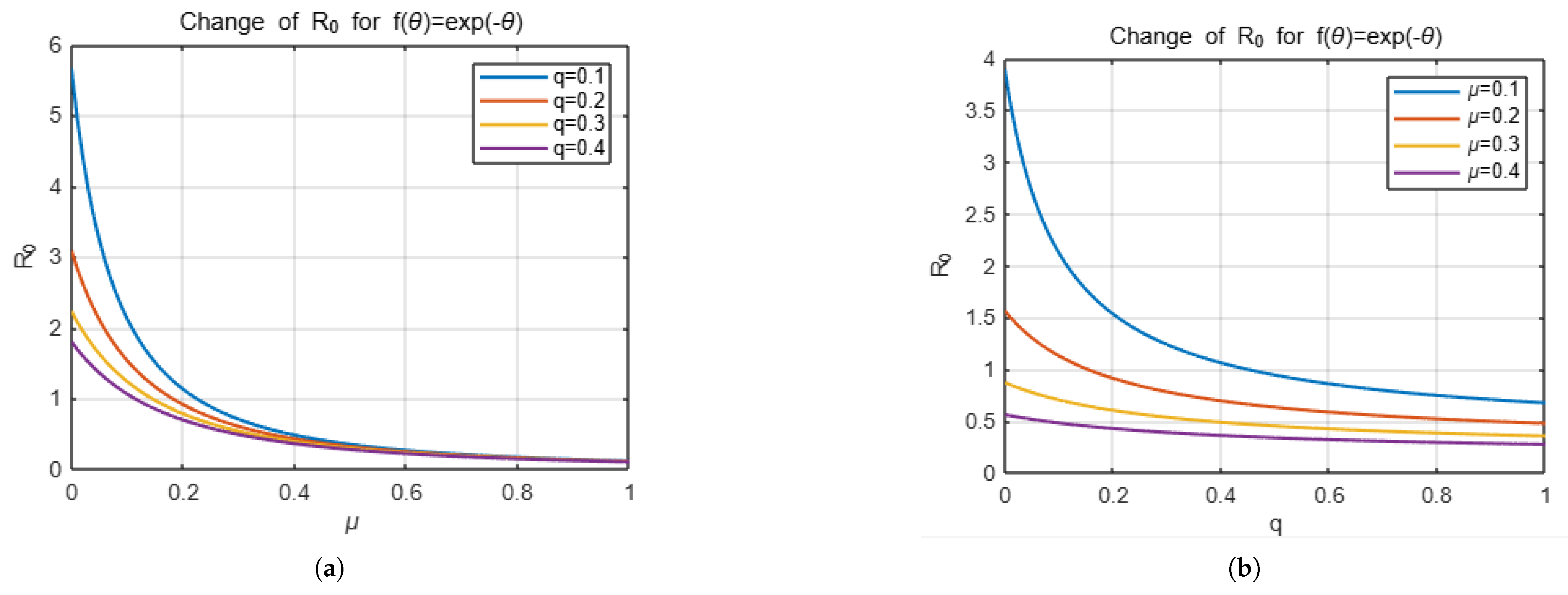
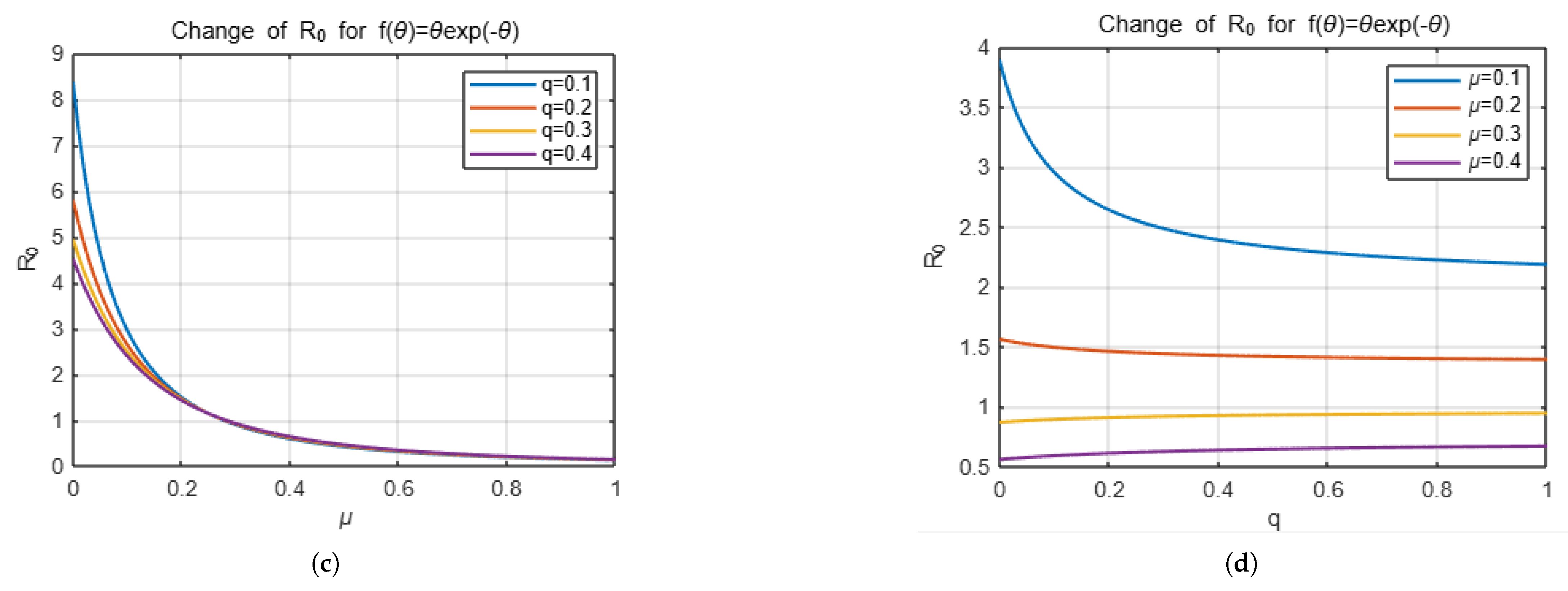
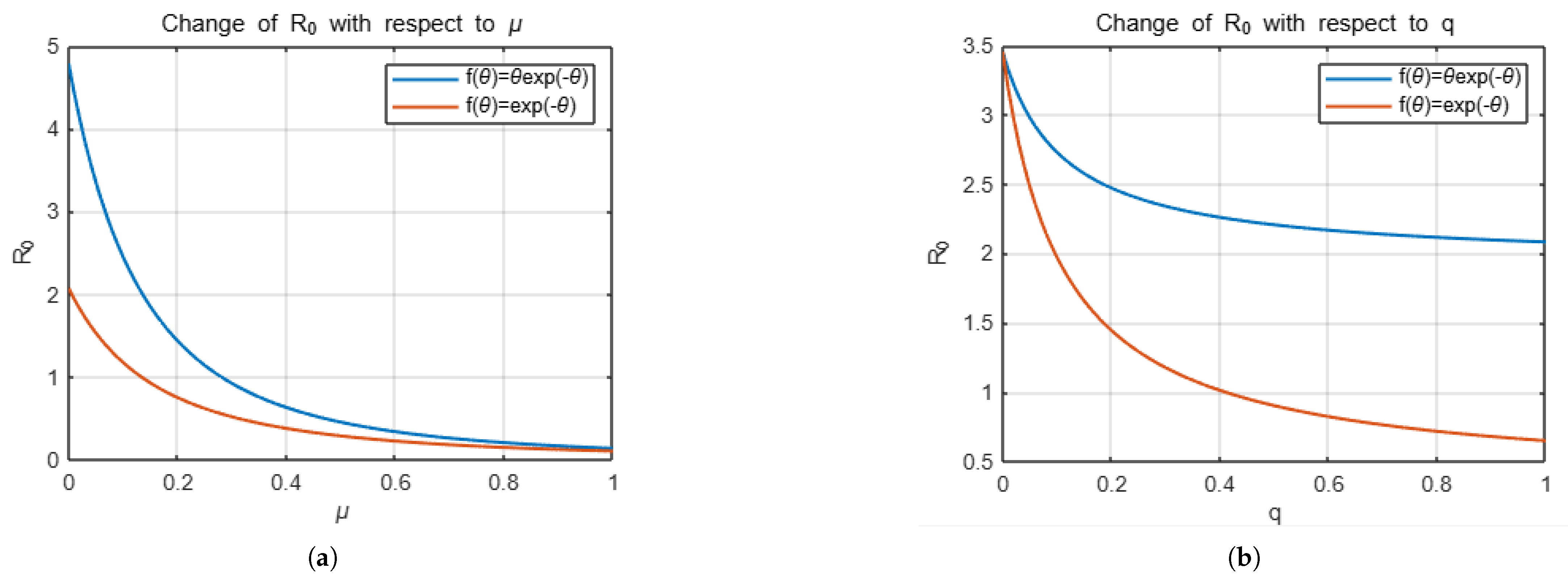
5. Some Examples for Distribution Function and ${\mathcal{R}}_{\mathbf{0}}$

Example 1. 

If we take the distribution function f as $f\left(\theta \right)=e^{-\theta }$, then

$$\underset{0}{\overset{\infty }{\int }}f\left(\theta \right)d\theta =1$$

and

$$\begin{array}{ccc}\hfill F& =& \underset{0}{\overset{\infty }{\int }}f\left(\theta \right)e^{-\mu \theta }d\theta =\underset{0}{\overset{\infty }{\int }}{e}^{-\left(\mu +1\right)\theta }d\theta \hfill \\ & =& \underset{t\to \infty }{lim}\underset{0}{\overset{t}{\int }}{e}^{-\left(\mu +1\right)\theta }d\theta =\underset{t\to \infty }{lim}\left({\displaystyle \frac{1-e^{-\left(\mu +1\right)t}}{\mu +1}}\right)={\displaystyle \frac{1}{\mu +1}}.\hfill \end{array}$$

Therefore, we obtain ${\mathcal{R}}_0$ as

$${\mathcal{R}}_0={\displaystyle \frac{b\beta \left(\mu +q+1\right)}{\left(q+\mu \right)\left(\gamma +\delta +\mu \right)\left(\mu +1\right)}}.$$

Example 2. 

If we take f as $f\left(\theta \right)=\theta e^{-\theta }$, then

$$\underset{0}{\overset{\infty }{\int }}f\left(\theta \right)d\theta =1$$

and we obtain

$$\begin{array}{ccc}\hfill F& =& \underset{0}{\overset{\infty }{\int }}f\left(\theta \right)e^{-\mu \theta }d\theta =\underset{0}{\overset{\infty }{\int }}\theta e^{-\left(\mu +1\right)\theta }d\theta \hfill \\ & =& \underset{t\to \infty }{lim}\underset{0}{\overset{t}{\int }}\theta e^{-\left(\mu +1\right)\theta }d\theta =\underset{t\to \infty }{lim}\left({\displaystyle \frac{1-e^{-\left(\mu +1\right)t}\left(\mu t+t+1\right)}{{\left(\mu +1\right)}^2}}\right)={\displaystyle \frac{1}{{\left(\mu +1\right)}^2}}.\hfill \end{array}$$

Therefore, we can write ${\mathcal{R}}_0$ as

$${\mathcal{R}}_0={\displaystyle \frac{b\beta \left({\left(\mu +1\right)}^2+q\right)}{\left(q+\mu \right)\left(\gamma +\delta +\mu \right){\left(\mu +1\right)}^2}}.$$

Now we will focus on presenting the effect of the choice of distribution function on the number of secondary infections ${\mathcal{R}}_0$ with some simulations. For this, we will present the effect of the variables q, which is related to vaccination, and $\mu$, which is decisive in the distribution function, which determine ${\mathcal{R}}_0$. The simulation below shows how the change in the parameters q and $\mu$, respectively, affects ${\mathcal{R}}_0$ for two different distribution functions, keeping the other parameters that determine ${\mathcal{R}}_0$ constant except for these two parameters.

In the rest of the article, we will use the following parameters given in [25] (

Table 1. Numerical values defined for Model (10). (The values based on the data are given in [25]).

Parameters:	q	$\mathit{\gamma }$	$\mathit{\beta }$	$\mathit{\delta }$	b	$\mathit{\mu }$
Values:	0.33	0.19	0.21	0.12	0.76	0.11

).

The Figure 1 and Figure 2 represent the changes in ${\mathcal{R}}_0$ with respect to the q and $\mu$ variables depending on the choices of f.

As mentioned in the previous section, parameters $q,\gamma ,\delta$ and $\mu$ exhibit negative indices, while $\beta ,F,b$ display positive indices.

Table 2. Sensitivity indices of ${\mathcal{R}}_0$ with respect to the parameters, for $f\left(\theta \right)=e^{-\theta }$.

q	$\mathit{\gamma }$	$\mathit{\beta }$	$\mathit{\delta }$	F	b	$\mathit{\mu }$
−0.1208	−0.4523	1	−0.2857	0.2291	1	−0.11

and Figure 3 reflect this case.

A small example can be given to explain the meaning of these values. As can be seen in Table 2, sensitivity indices of $\gamma$ and F are −0.4523 and 0.2291, respectively. This means that, if $\gamma$ is increased by 10%, then ${\mathcal{R}}_0$ is decreased by 4.523%. Similary, a 10% increase in F results in a 2.291% increase in ${\mathcal{R}}_0$.

6. Conclusions

In this study, a mathematical epidemic model reflecting that the protection period provided by the vaccine effect may vary from person to person is presented with its analysis. This novel $SVIR$ fractional epidemic model is formed by the aid of a system of distributed delay nonlinear Caputo fractional integro-differential equations.

Firstly, equilibrium points of formed system are found and the basic reproduction number of the model are determined as

$${\mathcal{R}}_0={\displaystyle \frac{b\beta \left(1+qF\right)}{\left(q+\mu \right)\left(\gamma +\delta +\mu \right)}}.$$

Thus, it is proved that System (10) has a unique disease-free equilibrium point $P_{DF}$ when ${\mathcal{R}}_0<1$ and there is a unique endemic equilibrium $P_E$ when ${\mathcal{R}}_0>1$. Moreover, it has been shown that, in a population with infectious individuals, the disease will never disappear when ${\mathcal{R}}_0>1$. Thus, it has been reinforced that the introduced model is consistent and that ${\mathcal{R}}_0$ is meaningful.

Additionally, the global behavior of System (10) was examined. Firstly, it is proved that all solutions of the system tend toward $P_{DF}$ by constituting the appropriate Lyapunov function for ${\mathcal{R}}_0<1.$ Then, when ${\mathcal{R}}_0>1$ and $\alpha =1$, the proof of global stability of $P_E$ has been presented by the Dulac criterion and the Poincaré–Bendixson theorem, which are commonly used in two-dimensional population models.

When the effect of the parameters in the model on ${\mathcal{R}}_0$, it can be seen that the parameters that can reduce ${\mathcal{R}}_0$ and can be controlled partially or completely are q and $\gamma .$

$\gamma$ is the recovery (or treatment) rate, and q is the vaccination rate. Controlling the vaccination rate (q) is both easier and less costly than the recovery rate ($\gamma$). In addition, considering that vaccinating the entire population may not be possible in real terms and is costly, knowing the minimum vaccination level that must be achieved to eliminate the disease is extremely important. In this study, a result is also given regarding the minimum vaccination rate that must be achieved to eliminate the disease.

Possible future work could consist of adding the optimal control problem to the model or using other derivative definitions. Additionally, authors working in the field of applied mathematics can conduct numerical simulations for the model and their comparative analysis.

References

1. Kermack, W.O.; McKendrick, A.G. A contributions to the mathematical theory of epidemics. Proc. R. Soc. A 1927, 115, 700–721. [Google Scholar]
2. Tyagi, S.; Martha, S.C.; Abbas, S.; Debbouche, A. Mathematical modeling and analysis for controlling the spread of infectious diseases. Chaos Soliton Fract. 2021, 144, 110707. [Google Scholar]
3. Çakan, S. Dynamic analysis of a mathematical model with health care capacity for COVID-19 pandemic. Chaos Soliton Fract. 2020, 139, 110033. [Google Scholar] [CrossRef]
4. Çakan, S. Mathematical analysis of local and global dynamics of a new epidemic model. Turk. J. Math. 2022, 46, 533–551. [Google Scholar]
5. Chauhan, S.; Misra, O.P.; Dhar, J. Stability Analysis of SIR Model with Vaccination. Am. J. Comput. Math. 2014, 4, 17–23. [Google Scholar]
6. Liu, X.; Takeuchi, Y.; Iwami, S. SVIR epidemic models with vaccination strategies. J. Theor. Biol. 2008, 253, 1–11. [Google Scholar]
7. Sekerci, Y.; Khoshnaw, S.H.A. The impact of vaccination strategy on the spatiotemporal pattern dynamics of a COVID-19 epidemic model. Eur. Phys. J. Plus 2024, 139, 1–15. [Google Scholar]
8. Gökçe, A.; Gürbüz, B.; Rendall, A.D. Dynamics of a mathematical model of virus spreading incorporating the effect of a vaccine. Nonlinear Anal. Real World Appl. 2024, 78, 104097. [Google Scholar] [CrossRef]
9. Hamdan, N.; Kılıçman, A. A fractional order SIR epidemic model for dengue transmission. Chaos Soliton Fract. 2018, 114, 55–62. [Google Scholar]
10. Ullah, S.; Khan, M.A.; Farooq, M. A fractional model for the dynamics of TB virus. Chaos Soliton Fract. 2018, 116, 63–71. [Google Scholar]
11. Özdemir, N.; Uçar, E.; Avcı, D. Dynamic analysis of a fractional SVIR system modeling an infectious disease. Facta Univ. Ser. Math. Inform. 2022, 37, 605–619. [Google Scholar]
12. Gökbulut, N.; Amilo, D. Kaymakamzade, B. Fractional SVIR Model for COVID-19 under Caputo Derivative. J. Biometry Stud. 2021, 1, 58–64. [Google Scholar]
13. Delavari, H.; Baleanu, D.; Sadati, J. Stability analysis of Caputo fractional-order nonlinear systems revisited. Nonlinear Dyn. 2012, 67, 2433–2439. [Google Scholar] [CrossRef]
14. Vargas-De-León, C. Volterra-type Lyapunov functions for fractional-order epidemic systems. Commun. Nonlinear Sci. Numer. Simul. 2015, 24, 75–85. [Google Scholar] [CrossRef]
15. Alqahtani, Z.; Almuneef, A.; DarAssi, M.H.; AbuHour, Y.; Al-arydah, M.T.; Safi, M.A.; Al-Hdaibat, B. Mathematical analysis of fractional Chlamydia pandemic model. Sci. Rep. 2024, 14, 31113. [Google Scholar]
16. El Hajji, M.; Sayari, S. Analysis of a Fractional-order “SVEIR” Epidemic Model with a General Nonlinear Saturated Incidence Rate in a Continuous Reactor. Asian Res. J. Math. 2019, 12, 1–17. [Google Scholar]
17. Almeida, R. Analysis of a fractional SEIR model with treatment. Appl. Math. Lett. 2018, 84, 56–62. [Google Scholar]
18. Matignon, D. Stability results for fractional differential equations with applications to control processing. Comput. Eng. Syst. Appl. 1996, 2, 952–956. [Google Scholar]
19. Lakshmikantham, S.; Leela, S.; Martynyuk, A.A. Stability Analysis of Nonlinear Systems; Marcel Dekker, Inc.: New York, NY, USA, 1989. [Google Scholar]
20. Kuang, Y. Delay Differential Equations: With Applications in Population Dynamics; Academic Press: New York, NY, USA, 1993. [Google Scholar]
21. Driessche, P.V.D.; Watmough, J. Reproduction numbers and sub-threshold endemic equilibria for compartmental models of disease transmission. Math. Biosci. 2002, 180, 29–48. [Google Scholar]
22. Rothman, K.J.; Lash, T.L.; Greenland, S. Modern Epidemiology, 3rd ed.; Lippincott Williams & Wilkins: Philadelphia, PA, USA, 2013. [Google Scholar]
23. Diethelm, K. Monotonocity of functions and sign changes of their Caputo derivatives. Fract. Calc. Appl. Anal. 2016, 19, 561–566. [Google Scholar]
24. Dulac, H. Recherche des cycles limites. C. R. Acad. Sci. Paris 1937, 204, 1703–1706. [Google Scholar]
25. Ismail, H.; Debbouche, A.; Hariharan, S.; Shangerganesh, L.; Kashtanova, S.V. Stability and Optimality Criteria for an SVIR Epidemic Model with Numerical Simulation. Mathematics 2024, 12, 3231. [Google Scholar] [CrossRef]
Figure 1. The variation of R 0 with respect to μ for different values of q for the selection of f ( θ ) = e θ f is shown in Figure (a). Here, the exception of the q and μ parameters are taken from [25]. (b) shows the variation of R 0 with respect to q for different values of μ . Additionally, for the f ( θ ) = θ e θ , these variations are presented in the forms of (c,d), respectively.
Fractalfract 09 00206 g001aFractalfract 09 00206 g001b
Figure 2. (a,b) represent the change in R 0 , for the choices f ( θ ) = e θ and f ( θ ) = θ e θ , with respect to μ and q, respectively.
Fractalfract 09 00206 g002
Figure 3. Plot represents the sensitivity of the parameters in the R 0 of the model.
Fractalfract 09 00206 g003