A Fractional Hybrid Staggered-Grid Grünwald–Letnikov Method for Numerical Simulation of Viscoelastic Seismic Wave Propagation

Abstract

The accurate and efficient simulation of seismic wave energy dissipation and phase dispersion during propagation in subsurface media due to inelastic attenuation is critical for the hydrocarbon-bearing distinction and improving the quality of seismic imaging in strongly attenuating geological media. The fractional viscoelastic equation, which quantifies frequency-independent anelastic effects, has recently become a focal point in seismic exploration. We have developed a novel hybrid staggered-grid Grünwald–Letnikov (HSGGL) finite difference method for solving the fractional viscoelastic equation in the time domain. The proposed method achieves accurate and computationally efficient solutions by using a staggered grid to discretize the first-order partial derivatives of the velocity–stress equations, combined with Grünwald–Letnikov finite difference discretization for the fractional-order terms. To improve the computational efficiency, we employ a preset accuracy to truncate the difference stencil, resulting in a compact fractional-order difference scheme. A stability analysis using the eigenvalue method reveals that the proposed method confers a relaxed stability condition, providing greater flexibility in the selection of sampling intervals. The numerical experiments indicate that the HSGGL method achieves a maximum relative error of no more than 0.17% compared to the reference solution (on a finely meshed domain) while being significantly faster than the conventional global FD method (GFD). In a 500 × 500 computational domain, the computation times for the proposed methods, which meet the specified accuracy levels used, are only approximately 4.67%, 4.47%, 4.44%, and 4.42% of that of the GFD method. This indicates that the novel HSGGL method has the potential as an effective forward modeling tool for understanding complex subsurface structures by employing a fractional viscoelastic equation.

1. Introduction

Seismic wave propagation attenuates in stratified media with viscous characteristics, possibly arising from overpressured free gas accumulations [1,2,3]. Consequently, the recorded seismic signals are significantly affected in their amplitude and phase, thereby further influencing the subsequent processes of reverse time migrations (RTMs) [4,5,6,7,8], full-waveform inversions (FWIs) [9,10,11], and amplitude-variation-with-offset (AVO) analyses [12] in the realm of oil and gas exploration. Thus, incorporating anelastic properties and accurately simulating wave propagation in the Earth is crucial.

The intrinsic seismic attenuation of strata is almost linearly related to the frequency within a limited band [13] and is mathematically represented by the approximating constant-Q model [14,15,16,17], the constant-Q viscoacoustic model [18,19,20,21] and the constant-Q viscoelastic model [22,23,24,25], reflecting a general consensus among geophysicists in recent years. Some studies rely on the memory characteristics of time fractional wave equations to describe the viscous effect [26,27,28,29]. Considering the limitations of substantial memory and hard disk storage, spatial fractional Laplacian operators [30] have been introduced into the constant-Q wave equation [15,31]. Carcione used the generalized spectral method to calculate the viscous acoustic wave equation [15]. Zhu and Harris [18] proposed a decoupled fractional Laplacian to separately describe amplitude loss and phase delay in the viscoacoustic wavefield using the pseudo-spectral (PS) method. Subsequently, Zhu and Carcione [22] extended it to the viscoelastic seismic wavefields but experienced serious simulation errors for sharp Q contrasts. Sun et al. [32] and Chen et al. [33] further proposed two viscoacoustic wave equations in terms of the constant fractional Laplacian, which simplifies the fast Fourier transform (FFT) simulations. To address the mixed-domain issue, Wang et al. [34] derived a spatial-independent-order decoupled fractional Laplacian viscoelastic equation based on the dispersion relation and simulated heterogeneous attenuating media using the PS method. Mu et al. [20,23] derived the decoupled fractional Laplacian viscoacoustic/viscoelastic formulation by inserting the complex-valued phase velocity into the frequency domain wave equation, which can be solved directly using the staggered-grid pseudospectral (SGPS) method. Zhang et al. [24] combined the relationship between the angular frequency and complex wavenumber to obtain a fractional Laplacian viscoelastic equation applicable to small Q media.

The aforementioned methods, relying on Fourier transform techniques to implement the variable-order fractional Laplacian in inhomogeneous media, reduce the efficiency of the simulations and inevitably introduce significant Gibbs effects [35,36]. Thus, Yao et al. [37] employed the Hermite distributed approximation functional (HDAF) method to handle the fractional viscoacoustic wave equation. Ji et al. [38] proposed a phase shift plus interpolation (PSPI) technique, which computes reference wavefields for a set of reference Qs and estimates the final wavefields using interpolation, with the aim of reducing the computational expense of the HDAF method. However, large-scale computations become challenging when the Q values exhibit significant variations. Gu et al. [36] derived difference coefficients by additionally using Fourier transforms based on the generating function integral expression, then employed a hybrid difference method to simulate viscoacoustic wave propagation. Song et al. [39] proposed an asymptotic local finite difference (ALFD) method with compact stencils that can be directly used to simulate fractional viscoacoustic wavefields. Nevertheless, finite difference methods capable of accurately and efficiently solving the fractional-order viscoelastic wave equation and simulating attenuated seismic wavefields have yet to be developed. This insight motivates us to develop the direct difference method for solving the viscoelastic equation. Considering the low programming complexity, high computational efficiency, and minimal storage requirements of finite difference (FD) methods for solving wave equations, along with the natural connection between the staggered-grid (SG) method and the velocity–stress formulation [27,40], we propose a hybrid finite difference method that combines the SG and Grünwald–Letnikov (GL) approaches to solve the spatial fractional viscoelastic equation.

In this paper, we commence by introducing the first-order viscoelastic equation, followed by a succinct overview of the SG discretization method. Subsequently, we propose a hybrid asymptotic local FD method, which combines SG and GL discretizations, featuring compact difference operators, to solve the fractional-order viscoelastic formula. Furthermore, we perform several types of analyses for the novel HSGGL, including stability conditions, numerical error evaluations, and efficiency comparisons, to demonstrate the accuracy and efficiency. Finally, we present several numerical simulations to further illustrate the applicability of this method in handling complex models, particularly those characterized by heterogeneous Q values.

2. Methodology

2.1. Viscoelastic Equation

We first briefly review the constant-Q model theory. According to the constant-Q model [27], the P-wave modulus M₀ and the S-wave modulus ${\mu }_0$ are given by

$$M_0=\rho c_{P_0}^2{\cos }^2\left(\pi {\gamma }_P/2\right),{\mu }_0=\rho c_{S_0}^2{\cos }^2\left(\pi {\gamma }_S/2\right),$$

(1)

where $c_{P0}$ and $c_{S0}$ are the P- and S-wave velocities at the reference frequency, respectively. The $\rho$ is the mass density and ${\gamma }_{P,S}=1/\pi {\tan }^{-1}\left(1/Q_{P,S}\right)$ is the fractional order, satisfying $0<\gamma <0.5$ for any positive value of Q. The stress–strain relation of the 2D case based on fractional spatial derivatives can be expressed as [22]

$${\sigma }_{xx}=\left[{\tau }_P{\displaystyle \frac{𝜕}{𝜕t}}{\left(-{\nabla }^2\right)}^{{\gamma }_P-1/2}+{\eta }_P{\left(-{\nabla }^2\right)}^{{\gamma }_P}\right]\left({\epsilon }_{xx}+{\epsilon }_{zz}\right)-2\left[{\tau }_S{\displaystyle \frac{𝜕}{𝜕t}}{\left(-{\nabla }^2\right)}^{{\gamma }_S-1/2}+{\eta }_S{\left(-{\nabla }^2\right)}^{{\gamma }_S}\right]{\epsilon }_{zz},$$

(2)

where ${\tau }_P=M_0{\omega }_0^{-2{\gamma }_p}{c}_{P_0}^{2{\gamma }_p-1}\sin \left(\pi {\gamma }_P\right),$ ${\eta }_P=M_0{\omega }_0^{-2{\gamma }_p}{c}_{P_0}^{2{\gamma }_p}\cos \left(\pi {\gamma }_P\right),$ ${\tau }_S={\mu }_0{\omega }_0^{-2{\gamma }_S}{c}_{S_0}^{2{\gamma }_S-1}\sin \left(\pi {\gamma }_S\right),$ ${\eta }_S={\mu }_0{\omega }_0^{-2{\gamma }_S}{c}_{S_0}^{2{\gamma }_S}\cos \left(\pi {\gamma }_S\right).$ Similarly, we have

$${\sigma }_{zz}=\left[{\tau }_P{\displaystyle \frac{𝜕}{𝜕t}}{\left(-{\nabla }^2\right)}^{{\gamma }_P-1/2}+{\eta }_P{\left(-{\nabla }^2\right)}^{{\gamma }_P}\right]\left({\epsilon }_{xx}+{\epsilon }_{zz}\right)-2\left[{\tau }_S{\displaystyle \frac{𝜕}{𝜕t}}{\left(-{\nabla }^2\right)}^{{\gamma }_S-1/2}+{\eta }_S{\left(-{\nabla }^2\right)}^{{\gamma }_S}\right]{\epsilon }_{xx},$$

(3)

$${\sigma }_{xz}=2{\tau }_S{\displaystyle \frac{𝜕}{𝜕t}}{\left(-{\nabla }^2\right)}^{{\gamma }_S-1/2}{\epsilon }_{xz}+2{\eta }_S{\left(-{\nabla }^2\right)}^{{\gamma }_S}{\epsilon }_{xz}.$$

(4)

respectively.

For a 2D elastic medium, the linear first-order momentum conservation equation can be written as

$$\rho {\displaystyle \frac{𝜕v_x}{𝜕t}}={\displaystyle \frac{𝜕{\sigma }_{xx}}{𝜕x}}+{\displaystyle \frac{𝜕{\sigma }_{xz}}{𝜕z}},$$

(5)

$$\rho {\displaystyle \frac{𝜕v_z}{𝜕t}}={\displaystyle \frac{𝜕{\sigma }_{zx}}{𝜕x}}+{\displaystyle \frac{𝜕{\sigma }_{zz}}{𝜕z}}.$$

(6)

The relationship between strain and velocity is

$${\displaystyle \frac{𝜕{\epsilon }_{xx}}{𝜕t}}={\displaystyle \frac{𝜕v_x}{𝜕x}},$$

(7)

$${\displaystyle \frac{𝜕{\epsilon }_{zz}}{𝜕t}}={\displaystyle \frac{𝜕v_z}{𝜕z}},$$

(8)

$${\displaystyle \frac{𝜕{\epsilon }_{xz}}{𝜕t}}={\displaystyle \frac{1}{2}}\left({\displaystyle \frac{𝜕v_z}{𝜕x}}+{\displaystyle \frac{𝜕v_x}{𝜕z}}\right).$$

(9)

Combining Formulas (2)–(9), the 2D fractional viscoelastic equation can be derived by the following first-order system:

$$\left\{\begin{array}{l}\rho {\displaystyle \frac{𝜕v_x}{𝜕t}}={\displaystyle \frac{𝜕{\sigma }_{xx}}{𝜕x}}+{\displaystyle \frac{𝜕{\sigma }_{xz}}{𝜕z}}+f_x\\ \rho {\displaystyle \frac{𝜕v_z}{𝜕t}}={\displaystyle \frac{𝜕{\sigma }_{zx}}{𝜕x}}+{\displaystyle \frac{𝜕{\sigma }_{zz}}{𝜕z}}+f_z\\ {\displaystyle \frac{𝜕{\sigma }_{xx}}{𝜕t}}={\tau }_P{\left(-{\nabla }^2\right)}^{{\gamma }_P-1/2}{\displaystyle \frac{𝜕}{𝜕t}}\left({\displaystyle \frac{𝜕v_x}{𝜕x}}+{\displaystyle \frac{𝜕v_z}{𝜕z}}\right)+{\eta }_P{\left(-{\nabla }^2\right)}^{{\gamma }_P}\left({\displaystyle \frac{𝜕v_x}{𝜕x}}+{\displaystyle \frac{𝜕v_z}{𝜕z}}\right)-2{\tau }_S{\left(-{\nabla }^2\right)}^{{\gamma }_S-1/2}{\displaystyle \frac{𝜕}{𝜕t}}{\displaystyle \frac{𝜕v_z}{𝜕z}}-2{\eta }_S{\left(-{\nabla }^2\right)}^{{\gamma }_S}{\displaystyle \frac{𝜕v_z}{𝜕z}}\\ {\displaystyle \frac{𝜕{\sigma }_{zz}}{𝜕t}}={\tau }_P{\left(-{\nabla }^2\right)}^{{\gamma }_P-1/2}{\displaystyle \frac{𝜕}{𝜕t}}\left({\displaystyle \frac{𝜕v_x}{𝜕x}}+{\displaystyle \frac{𝜕v_z}{𝜕z}}\right)+{\eta }_P{\left(-{\nabla }^2\right)}^{{\gamma }_P}\left({\displaystyle \frac{𝜕v_x}{𝜕x}}+{\displaystyle \frac{𝜕v_z}{𝜕z}}\right)-2{\tau }_S{\left(-{\nabla }^2\right)}^{{\gamma }_S-1/2}{\displaystyle \frac{𝜕}{𝜕t}}{\displaystyle \frac{𝜕v_x}{𝜕x}}-2{\eta }_S{\left(-{\nabla }^2\right)}^{{\gamma }_S}{\displaystyle \frac{𝜕v_x}{𝜕x}}\\ {\displaystyle \frac{𝜕{\sigma }_{xz}}{𝜕t}}={\tau }_S{\left(-{\nabla }^2\right)}^{{\gamma }_S-1/2}{\displaystyle \frac{𝜕}{𝜕t}}\left({\displaystyle \frac{𝜕v_x}{𝜕x}}+{\displaystyle \frac{𝜕v_z}{𝜕z}}\right)+{\eta }_S{\left(-{\nabla }^2\right)}^{{\gamma }_S}\left({\displaystyle \frac{𝜕v_x}{𝜕x}}+{\displaystyle \frac{𝜕v_z}{𝜕z}}\right)\end{array}\right.,$$

(10)

where $v_x$ and $v_z$ represent the particle velocity components in the x- and z-directions, respectively; ${\sigma }_{xx}$, ${\sigma }_{zz}$, and ${\sigma }_{xz}$ are the stress components; and $f_x$ and $f_z$ are the body force. When $Q_{P,S}\to \infty$ (${\gamma }_{P,S}\to 0$), we obtain the elastic case.

2.2. Hybrid Stagged-Grid Grünwald–Letnikov (SGGL) Finite Difference Method

Firstly, we discretize the first-order velocity–stress equation in Equation (10) using the SGFD method as follows:

$$\left\{\begin{array}{l}{\left(v_x\right)}_{i+{\displaystyle \frac{1}{2}},j}^{t+{\displaystyle \frac{1}{2}}}={\left(v_x\right)}_{i+{\displaystyle \frac{1}{2}},j}^{t-{\displaystyle \frac{1}{2}}}+{\displaystyle \frac{\Delta t}{\Delta x\rho }}{\displaystyle \sum _{n=1}^N{C}_n^{\left(N\right)}\left[{\left({\sigma }_{xx}\right)}_{i+n,j}^t-{\left({\sigma }_{xx}\right)}_{i-\left(n-1\right),j}^t\right]}+{\displaystyle \frac{\Delta t}{\Delta z\rho }}{\displaystyle \sum _{n=1}^N{C}_n^{\left(N\right)}\left[{\left({\sigma }_{xz}\right)}_{i+\frac{1}{2},j+\frac{2n-1}{2}}^t-{\left({\sigma }_{xz}\right)}_{i+\frac{1}{2},j-\frac{2n-1}{2}}^t\right]}\\ {\left(v_z\right)}_{i,j+{\displaystyle \frac{1}{2}}}^{t+{\displaystyle \frac{1}{2}}}={\left(v_z\right)}_{i,j+{\displaystyle \frac{1}{2}}}^{t-{\displaystyle \frac{1}{2}}}+{\displaystyle \frac{\Delta t}{\Delta x\rho }}{\displaystyle \sum _{n=1}^N{C}_n^{\left(N\right)}\left[{\left({\sigma }_{zx}\right)}_{i+\frac{2n-1}{2},j+\frac{1}{2}}^t-{\left({\sigma }_{zx}\right)}_{i-\frac{2n-1}{2},j+\frac{1}{2}}^t\right]}+{\displaystyle \frac{\Delta t}{\Delta z\rho }}{\displaystyle \sum _{n=1}^N{C}_n^{\left(N\right)}\left[{\left({\sigma }_{zz}\right)}_{i,j+n}^t-{\left({\sigma }_{zz}\right)}_{i,j-\left(n-1\right)}^t\right]}\end{array}\right.,$$

(11)

$C_n^{\left(N\right)}$ is the differential coefficient of the SG method; we will set $N=2$, then $C_1^{\left(2\right)}=1.125$ and $C_2^{\left(2\right)}=-0.04167$. Next, we use the GL method [26,27] to discretize the fractional order terms. The fractional derivative of a function $u\left(x\right)$ is

$${\displaystyle \frac{{𝜕}^{\alpha }u}{𝜕x^{\alpha }}}={\displaystyle \frac{1}{h^{\alpha }}}{\displaystyle \sum _{m=0}^{\infty }{\left(-1\right)}^m\left(\begin{array}{c}\alpha \\ m\end{array}\right)u\left(x-mh\right)}.$$

(12)

At this stage, by denoting ${\left(-1\right)}^m\left(\begin{array}{c}\alpha \\ m\end{array}\right)$ as $g_m^{\alpha }$, we can further discretize Equation (10) into

$$\left\{\begin{array}{l}{\left({\sigma }_{xx}\right)}_{i,j}^{t+1}={\left({\sigma }_{xx}\right)}_{i,j}^t+{\displaystyle \frac{{\tau }_P}{\Delta x^{2{\gamma }_P}}}{\displaystyle \sum _{m=-\infty }^{\infty }{g}_m^{2{\gamma }_P}}\left[{\left(v_x\right)}_{i+{\displaystyle \frac{1}{2}}-m,j}^{t+{\displaystyle \frac{1}{2}}}-{\left(v_x\right)}_{i+{\displaystyle \frac{1}{2}}-m,j}^{t-{\displaystyle \frac{1}{2}}}\right]+{\displaystyle \frac{{\tau }_P}{\Delta z^{2{\gamma }_P}}}{\displaystyle \sum _{n=-\infty }^{\infty }{g}_n^{2{\gamma }_P}}\left[{\left(v_z\right)}_{i,j+{\displaystyle \frac{1}{2}}-n}^{t+{\displaystyle \frac{1}{2}}}-{\left(v_z\right)}_{i,j+{\displaystyle \frac{1}{2}}-n}^{t-{\displaystyle \frac{1}{2}}}\right]\\ +\Delta t{\eta }_P\left[{\displaystyle \frac{1}{\Delta x^{2{\gamma }_P+1}}}{\displaystyle \sum _{m=-\infty }^{\infty }{g}_m^{\left(2{\gamma }_P+1\right)}}{\left(v_x\right)}_{i+{\displaystyle \frac{1}{2}}-m,j}^{t+{\displaystyle \frac{1}{2}}}+{\displaystyle \frac{1}{\Delta z^{2{\gamma }_P+1}}}{\displaystyle \sum _{n=-\infty }^{\infty }{g}_n^{\left(2{\gamma }_P+1\right)}}{\left(v_z\right)}_{i,j+{\displaystyle \frac{1}{2}}-n}^{t+{\displaystyle \frac{1}{2}}}\right]-{\displaystyle \frac{2{\tau }_S}{\Delta z^{2{\gamma }_S}}}{\displaystyle \sum _{n=-\infty }^{\infty }{g}_n^{2{\gamma }_S}}\left[{\left(v_z\right)}_{i,j+{\displaystyle \frac{1}{2}}-n}^{t+{\displaystyle \frac{1}{2}}}-{\left(v_z\right)}_{i,j+{\displaystyle \frac{1}{2}}-n}^{t-{\displaystyle \frac{1}{2}}}\right]-{\displaystyle \frac{2\Delta t{\eta }_S}{\Delta z^{2{\gamma }_S+1}}}{\displaystyle \sum _{n=-\infty }^{\infty }{g}_n^{\left(2{\gamma }_S+1\right)}}{\left(v_z\right)}_{i,j+{\displaystyle \frac{1}{2}}-n}^{t+{\displaystyle \frac{1}{2}}}\\ {\left({\sigma }_{zz}\right)}_{i,j}^{t+1}={\left({\sigma }_{zz}\right)}_{i,j}^t+{\displaystyle \frac{{\tau }_P}{\Delta x^{2{\gamma }_P}}}{\displaystyle \sum _{m=-\infty }^{\infty }{g}_m^{2{\gamma }_P}}\left[{\left(v_x\right)}_{i+{\displaystyle \frac{1}{2}}-m,j}^{t+{\displaystyle \frac{1}{2}}}-{\left(v_x\right)}_{i+{\displaystyle \frac{1}{2}}-m,j}^{t-{\displaystyle \frac{1}{2}}}\right]+{\displaystyle \frac{{\tau }_P}{\Delta z^{2{\gamma }_P}}}{\displaystyle \sum _{n=-\infty }^{\infty }{g}_n^{2{\gamma }_P}}\left[{\left(v_z\right)}_{i,j+{\displaystyle \frac{1}{2}}-n}^{t+{\displaystyle \frac{1}{2}}}-{\left(v_z\right)}_{i,j+{\displaystyle \frac{1}{2}}-n}^{t-{\displaystyle \frac{1}{2}}}\right]\\ +\Delta t{\eta }_P\left[{\displaystyle \frac{1}{\Delta x^{2{\gamma }_P+1}}}{\displaystyle \sum _{m=-\infty }^{\infty }{g}_m^{\left(2{\gamma }_P+1\right)}}{\left(v_x\right)}_{i+{\displaystyle \frac{1}{2}}-m,j}^{t+{\displaystyle \frac{1}{2}}}+{\displaystyle \frac{1}{\Delta z^{2{\gamma }_P+1}}}{\displaystyle \sum _{n=-\infty }^{\infty }{g}_n^{\left(2{\gamma }_P+1\right)}}{\left(v_z\right)}_{i,j+{\displaystyle \frac{1}{2}}-n}^{t+{\displaystyle \frac{1}{2}}}\right]-{\displaystyle \frac{2{\tau }_S}{\Delta x^{2{\gamma }_S}}}{\displaystyle \sum _{m=-\infty }^{\infty }{g}_m^{2{\gamma }_S}}\left[{\left(v_x\right)}_{i+{\displaystyle \frac{1}{2}}-m,j}^{t+{\displaystyle \frac{1}{2}}}-{\left(v_x\right)}_{i+{\displaystyle \frac{1}{2}}-m,j}^{t-{\displaystyle \frac{1}{2}}}\right]-{\displaystyle \frac{2\Delta t{\eta }_S}{\Delta x^{2{\gamma }_S+1}}}{\displaystyle \sum _{m=-\infty }^{\infty }{g}_m^{\left(2{\gamma }_S+1\right)}}{\left(v_x\right)}_{i+{\displaystyle \frac{1}{2}}-m,j}^{t+{\displaystyle \frac{1}{2}}}\\ {\left({\sigma }_{xz}\right)}_{i,j}^{t+1}={\displaystyle \frac{{\tau }_S}{\Delta z^{2{\gamma }_S}}}{\displaystyle \sum _{n=-\infty }^{\infty }{g}_n^{2{\gamma }_S}}\left[{\left(v_x\right)}_{i+{\displaystyle \frac{1}{2}},j-n}^{t+{\displaystyle \frac{1}{2}}}-{\left(v_x\right)}_{i+{\displaystyle \frac{1}{2}},j-n}^{t-{\displaystyle \frac{1}{2}}}\right]+{\displaystyle \frac{{\tau }_S}{\Delta x^{2{\gamma }_S}}}{\displaystyle \sum _{m=-\infty }^{\infty }{g}_m^{2{\gamma }_S}}\left[{\left(v_z\right)}_{i-m,j+{\displaystyle \frac{1}{2}}}^{t+{\displaystyle \frac{1}{2}}}-{\left(v_z\right)}_{i-m,j+{\displaystyle \frac{1}{2}}}^{t-{\displaystyle \frac{1}{2}}}\right]\\ +\Delta t{\eta }_S\left[{\displaystyle \frac{1}{\Delta z^{2{\gamma }_S+1}}}{\displaystyle \sum _{n=-\infty }^{\infty }{g}_n^{\left(2{\gamma }_S+1\right)}}{\left(v_x\right)}_{i+{\displaystyle \frac{1}{2}},j-n}^{t+{\displaystyle \frac{1}{2}}}+{\displaystyle \frac{1}{\Delta x^{2{\gamma }_S+1}}}{\displaystyle \sum _{m=-\infty }^{\infty }{g}_m^{\left(2{\gamma }_S+1\right)}}{\left(v_z\right)}_{i-m,j+{\displaystyle \frac{1}{2}}}^{t+{\displaystyle \frac{1}{2}}}\right]\end{array}\right..$$

(13)

We obtained a hybrid global SGGL (GSGGL) method as Formula (13). In fact, we can utilize the property that the difference coefficients rapidly decay to zero as the displacement offset m and n increases to obtain sufficiently accurate asymptotic local approximations [37,39]. Therefore, we rewrite the expression as

$$\left\{\begin{array}{l}{\left({\sigma }_{xx}\right)}_{i,j}^{t+1}={\left({\sigma }_{xx}\right)}_{i,j}^t+{\displaystyle \frac{{\tau }_P}{\Delta x^{2{\gamma }_P}}}{\displaystyle \sum _{m=-M_{\epsilon ,\gamma }}^{M_{\epsilon ,\gamma }}{g}_m^{2{\gamma }_P}}\left[{\left(v_x\right)}_{i+{\displaystyle \frac{1}{2}}-m,j}^{t+{\displaystyle \frac{1}{2}}}-{\left(v_x\right)}_{i+{\displaystyle \frac{1}{2}}-m,j}^{t-{\displaystyle \frac{1}{2}}}\right]+{\displaystyle \frac{{\tau }_P}{\Delta z^{2{\gamma }_P}}}{\displaystyle \sum _{n=-N_{\epsilon ,\gamma }}^{N_{\epsilon ,\gamma }}{g}_n^{2{\gamma }_P}}\left[{\left(v_z\right)}_{i,j+{\displaystyle \frac{1}{2}}-n}^{t+{\displaystyle \frac{1}{2}}}-{\left(v_z\right)}_{i,j+{\displaystyle \frac{1}{2}}-n}^{t-{\displaystyle \frac{1}{2}}}\right]\\ +\Delta t{\eta }_P\left[{\displaystyle \frac{1}{\Delta x^{2{\gamma }_P+1}}}{\displaystyle \sum _{m=-M_{\epsilon ,\gamma }}^{M_{\epsilon ,\gamma }}{g}_m^{\left(2{\gamma }_P+1\right)}}{\left(v_x\right)}_{i+{\displaystyle \frac{1}{2}}-m,j}^{t+{\displaystyle \frac{1}{2}}}+{\displaystyle \frac{1}{\Delta z^{2{\gamma }_P+1}}}{\displaystyle \sum _{n=-N_{\epsilon ,\gamma }}^{N_{\epsilon ,\gamma }}{g}_n^{\left(2{\gamma }_P+1\right)}}{\left(v_z\right)}_{i,j+{\displaystyle \frac{1}{2}}-n}^{t+{\displaystyle \frac{1}{2}}}\right]-{\displaystyle \frac{2{\tau }_S}{\Delta z^{2{\gamma }_S}}}{\displaystyle \sum _{n=-N_{\epsilon ,\gamma }}^{N_{\epsilon ,\gamma }}{g}_n^{2{\gamma }_S}}\left[{\left(v_z\right)}_{i,j+{\displaystyle \frac{1}{2}}-n}^{t+{\displaystyle \frac{1}{2}}}-{\left(v_z\right)}_{i,j+{\displaystyle \frac{1}{2}}-n}^{t-{\displaystyle \frac{1}{2}}}\right]-{\displaystyle \frac{2\Delta t{\eta }_S}{\Delta z^{2{\gamma }_S+1}}}{\displaystyle \sum _{n=-N_{\epsilon ,\gamma }}^{N_{\epsilon ,\gamma }}{g}_n^{\left(2{\gamma }_S+1\right)}}{\left(v_z\right)}_{i,j+{\displaystyle \frac{1}{2}}-n}^{t+{\displaystyle \frac{1}{2}}}\\ {\left({\sigma }_{zz}\right)}_{i,j}^{t+1}={\left({\sigma }_{zz}\right)}_{i,j}^t+{\displaystyle \frac{{\tau }_P}{\Delta x^{2{\gamma }_P}}}{\displaystyle \sum _{m=-M_{\epsilon ,\gamma }}^{M_{\epsilon ,\gamma }}{g}_m^{2{\gamma }_P}}\left[{\left(v_x\right)}_{i+{\displaystyle \frac{1}{2}}-m,j}^{t+{\displaystyle \frac{1}{2}}}-{\left(v_x\right)}_{i+{\displaystyle \frac{1}{2}}-m,j}^{t-{\displaystyle \frac{1}{2}}}\right]+{\displaystyle \frac{{\tau }_P}{\Delta z^{2{\gamma }_P}}}{\displaystyle \sum _{n=-N_{\epsilon ,\gamma }}^{N_{\epsilon ,\gamma }}{g}_n^{2{\gamma }_P}}\left[{\left(v_z\right)}_{i,j+{\displaystyle \frac{1}{2}}-n}^{t+{\displaystyle \frac{1}{2}}}-{\left(v_z\right)}_{i,j+{\displaystyle \frac{1}{2}}-n}^{t-{\displaystyle \frac{1}{2}}}\right]\\ +\Delta t{\eta }_P\left[{\displaystyle \frac{1}{\Delta x^{2{\gamma }_P+1}}}{\displaystyle \sum _{m=-M_{\epsilon ,\gamma }}^{M_{\epsilon ,\gamma }}{g}_m^{\left(2{\gamma }_P+1\right)}}{\left(v_x\right)}_{i+{\displaystyle \frac{1}{2}}-m,j}^{t+{\displaystyle \frac{1}{2}}}+{\displaystyle \frac{1}{\Delta z^{2{\gamma }_P+1}}}{\displaystyle \sum _{n=-N_{\epsilon ,\gamma }}^{N_{\epsilon ,\gamma }}{g}_n^{\left(2{\gamma }_P+1\right)}}{\left(v_z\right)}_{i,j+{\displaystyle \frac{1}{2}}-n}^{t+{\displaystyle \frac{1}{2}}}\right]-{\displaystyle \frac{2{\tau }_S}{\Delta x^{2{\gamma }_S}}}{\displaystyle \sum _{m=-M_{\epsilon ,\gamma }}^{M_{\epsilon ,\gamma }}{g}_m^{2{\gamma }_S}}\left[{\left(v_x\right)}_{i+{\displaystyle \frac{1}{2}}-m,j}^{t+{\displaystyle \frac{1}{2}}}-{\left(v_x\right)}_{i+{\displaystyle \frac{1}{2}}-m,j}^{t-{\displaystyle \frac{1}{2}}}\right]-{\displaystyle \frac{2\Delta t{\eta }_S}{\Delta x^{2{\gamma }_S+1}}}{\displaystyle \sum _{m=-M_{\epsilon ,\gamma }}^{M_{\epsilon ,\gamma }}{g}_m^{\left(2{\gamma }_S+1\right)}}{\left(v_x\right)}_{i+{\displaystyle \frac{1}{2}}-m,j}^{t+{\displaystyle \frac{1}{2}}}\\ {\left({\sigma }_{xz}\right)}_{i,j}^{t+1}={\displaystyle \frac{{\tau }_S}{\Delta z^{2{\gamma }_S}}}{\displaystyle \sum _{n=-N_{\epsilon ,\gamma }}^{N_{\epsilon ,\gamma }}{g}_n^{2{\gamma }_S}}\left[{\left(v_x\right)}_{i+{\displaystyle \frac{1}{2}},j-n}^{t+{\displaystyle \frac{1}{2}}}-{\left(v_x\right)}_{i+{\displaystyle \frac{1}{2}},j-n}^{t-{\displaystyle \frac{1}{2}}}\right]+{\displaystyle \frac{{\tau }_S}{\Delta x^{2{\gamma }_S}}}{\displaystyle \sum _{m=-M_{\epsilon ,\gamma }}^{M_{\epsilon ,\gamma }}{g}_m^{2{\gamma }_S}}\left[{\left(v_z\right)}_{i-m,j+{\displaystyle \frac{1}{2}}}^{t+{\displaystyle \frac{1}{2}}}-{\left(v_z\right)}_{i-m,j+{\displaystyle \frac{1}{2}}}^{t-{\displaystyle \frac{1}{2}}}\right]\\ +\Delta t{\eta }_S\left[{\displaystyle \frac{1}{\Delta z^{2{\gamma }_S+1}}}{\displaystyle \sum _{n=-N_{\epsilon ,\gamma }}^{N_{\epsilon ,\gamma }}{g}_n^{\left(2{\gamma }_S+1\right)}}{\left(v_x\right)}_{i+{\displaystyle \frac{1}{2}},j-n}^{t+{\displaystyle \frac{1}{2}}}+{\displaystyle \frac{1}{\Delta x^{2{\gamma }_S+1}}}{\displaystyle \sum _{m=-M_{\epsilon ,\gamma }}^{M_{\epsilon ,\gamma }}{g}_m^{\left(2{\gamma }_S+1\right)}}{\left(v_z\right)}_{i-m,j+{\displaystyle \frac{1}{2}}}^{t+{\displaystyle \frac{1}{2}}}\right]\end{array}\right..$$

(14)

The parameters $M_{\epsilon ,\gamma }$ and $N_{\epsilon ,\gamma }$ of the differential stencil is determined by the operator truncation error $\epsilon$ and the Q-value, such that for any given error $\epsilon >0$, there exists the minimum differential stencil $M_{\epsilon ,\gamma }$ required to achieve different accuracy under different quality factors Q (or fractional order $\gamma$) (

Table 1. Minimum differential stencil $M_{\epsilon ,\gamma }$ required under different truncation error limits.

Truncated Relative Error $\mathit{\epsilon }$
QP	10 × 10−2	10 × 10−3	10 × 10−4	10 × 10−5
$120({\gamma }_P=0.0027$)	2	3	8	24
$40({\gamma }_P=0.0079$)	3	5	13	40
$32({\gamma }_P=0.0099$)	3	5	15	44
$20({\gamma }_P=0.0159$)	4	7	18	54
$12({\gamma }_P=0.0265$)	4	8	22	67
$10({\gamma }_P=0.0317$)	5	9	24	71

) for the asymptotic local HSGGL (ALHSGGL) scheme [39]. Thus, the discrete form of the fractional viscoelastic motion equation can be obtained using Expressions (11) and (14) and Table 1. For example, the given truncation error under $Q_p=32$($Q_S=Q_P/\sqrt{3}$) is $\epsilon <{10}^{-4}$; thus, the minimum difference length of the P-wave is $M_{\epsilon ,\gamma }=15$, and the minimum difference length of the S-wave is $N_{\epsilon ,\gamma }=19$. Next, we can obtain the discrete form of the ALHSGGL scheme as follows:

$$\begin{array}{l}{\left({\sigma }_{xx}\right)}_{i,j}^{t+1}={\left({\sigma }_{xx}\right)}_{i,j}^t+{\displaystyle \frac{{\tau }_P}{\Delta x^{2{\gamma }_P}}}{\displaystyle \sum _{m=-15}^{15}{g}_m^{2{\gamma }_P}}\left[{\left(v_x\right)}_{i+{\displaystyle \frac{1}{2}}-m,j}^{t+{\displaystyle \frac{1}{2}}}-{\left(v_x\right)}_{i+{\displaystyle \frac{1}{2}}-m,j}^{t-{\displaystyle \frac{1}{2}}}\right]+{\displaystyle \frac{{\tau }_P}{\Delta z^{2{\gamma }_P}}}{\displaystyle \sum _{n=-15}^{15}{g}_n^{2{\gamma }_P}}\left[{\left(v_z\right)}_{i,j+{\displaystyle \frac{1}{2}}-n}^{t+{\displaystyle \frac{1}{2}}}-{\left(v_z\right)}_{i,j+{\displaystyle \frac{1}{2}}-n}^{t-{\displaystyle \frac{1}{2}}}\right]\\ \hspace{1em}\hspace{1em}+\Delta t{\eta }_P\left[{\displaystyle \frac{1}{\Delta x^{2{\gamma }_P+1}}}{\displaystyle \sum _{m=-15}^{15}{g}_m^{\left(2{\gamma }_P+1\right)}}{\left(v_x\right)}_{i+{\displaystyle \frac{1}{2}}-m,j}^{t+{\displaystyle \frac{1}{2}}}+{\displaystyle \frac{1}{\Delta z^{2{\gamma }_P+1}}}{\displaystyle \sum _{n=-15}^{15}{g}_n^{\left(2{\gamma }_P+1\right)}}{\left(v_z\right)}_{i,j+{\displaystyle \frac{1}{2}}-n}^{t+{\displaystyle \frac{1}{2}}}\right]\\ \hspace{1em}\hspace{1em}-{\displaystyle \frac{2{\tau }_S}{\Delta z^{2{\gamma }_S}}}{\displaystyle \sum _{n=-19}^{19}{g}_n^{2{\gamma }_S}}\left[{\left(v_z\right)}_{i,j+{\displaystyle \frac{1}{2}}-n}^{t+{\displaystyle \frac{1}{2}}}-{\left(v_z\right)}_{i,j+{\displaystyle \frac{1}{2}}-n}^{t-{\displaystyle \frac{1}{2}}}\right]-{\displaystyle \frac{2\Delta t{\eta }_S}{\Delta z^{2{\gamma }_S+1}}}{\displaystyle \sum _{n=-19}^{19}{g}_n^{\left(2{\gamma }_S+1\right)}}{\left(v_z\right)}_{i,j+{\displaystyle \frac{1}{2}}-n}^{t+{\displaystyle \frac{1}{2}}}.\end{array}$$

(15)

2.3. Stability Analysis

In this section, we use the Fourier method to analyze the numerical stability of the ALSGGL method. By introducing the harmonic solution $u_{i,j}^n={\psi }_r\exp \left[I\left(ih{k}_x+jh{k}_z-k{c}^{\prime }n\Delta t\right)\right]$ ($r=1,2,3,4,5$), substituting it into the difference scheme in Expressions (11) and (14), and setting $\Delta x=\Delta z=h$, we obtain

$$\left[\begin{array}{c}\begin{array}{c}{\psi }_1\\ {\psi }_2\end{array}\\ {\psi }_3\\ \begin{array}{c}{\psi }_4\\ {\psi }_5\end{array}\end{array}\right]\xi =\left[\begin{array}{ccccc}0& 0& {\alpha }_0{X}_0& 0& {\alpha }_0{Z}_0\\ 0& 0& 0& {\alpha }_0{Z}_0& {\alpha }_0{X}_0\\ P_1{X}_1+P_2{X}_2& P_1{Z}_1+P_2{Z}_2-2S_1{Z}_1-2S_2{Z}_2& 0& 0& 0\\ P_1{X}_1+P_2{X}_2-2S_1{X}_1-2S_2{X}_2& P_1{Z}_1+P_2{Z}_2& 0& 0& 0\\ S_{1}Z{X}_1+S_{2}Z{X}_2& S_{1}X{Z}_1+S_{2}X{Z}_2& 0& 0& 0\end{array}\right]\left[\begin{array}{c}\begin{array}{c}{\psi }_1\\ {\psi }_2\end{array}\\ {\psi }_3\\ \begin{array}{c}{\psi }_4\\ {\psi }_5\end{array}\end{array}\right].$$

(16)

where, $\xi =\sin {\displaystyle \frac{kc\prime \Delta t}{2}}$, ${\alpha }_0={\displaystyle \frac{\Delta t}{h\rho }}$, $P_1={\displaystyle \frac{{\tau }_P}{h^{2{\gamma }_P}}}$, $P_2={\displaystyle \frac{\Delta t{\eta }_P}{h^{2{\gamma }_P+1}}}$, $S_1={\displaystyle \frac{{\tau }_S}{h^{2{\gamma }_S}}}$, $S_2={\displaystyle \frac{\Delta t{\eta }_S}{h^{2{\gamma }_S+1}}}$;

$$X_0=C_1^{\left(2\right)}\sin \left({\displaystyle \frac{h{k}_x}{2}}\right)+C_2^{\left(2\right)}\sin \left({\displaystyle \frac{3h{k}_x}{2}}\right)=1.125\sin \left({\displaystyle \frac{h{k}_x}{2}}\right)-0.04167\sin \left({\displaystyle \frac{3h{k}_x}{2}}\right)$$

(17)

$$Z_0=C_1^{\left(2\right)}\sin \left({\displaystyle \frac{h{k}_z}{2}}\right)+C_2^{\left(2\right)}\sin \left({\displaystyle \frac{3h{k}_z}{2}}\right)=1.125\sin \left({\displaystyle \frac{h{k}_z}{2}}\right)-0.04167\sin \left({\displaystyle \frac{3h{k}_z}{2}}\right)$$

(18)

$$X_1={\displaystyle \sum _{m=-\infty }^{\infty }{g}_m^{2{\gamma }_P}}\left[\cos {\displaystyle \frac{\left(1-2m\right)h{k}_x}{2}}+I\sin {\displaystyle \frac{\left(1-2m\right)h{k}_x}{2}}\right]\left[\sin {\displaystyle \frac{k{c}^{\prime }\Delta t}{2}}\right]$$

(19)

$$X_2={\displaystyle \sum _{m=-\infty }^{\infty }{g}_m^{\left(2{\gamma }_P+1\right)}}\left[I\cos {\displaystyle \frac{\left(1-2m\right)h{k}_x}{2}}-\sin {\displaystyle \frac{\left(1-2m\right)h{k}_x}{2}}\right]$$

(20)

$$Z_1={\displaystyle \sum _{n=-\infty }^{\infty }{g}_n^{2{\gamma }_P}}\left[\cos {\displaystyle \frac{\left(1-2n\right)h{k}_z}{2}}+I\sin {\displaystyle \frac{\left(1-2n\right)h{k}_z}{2}}\right]\left[\sin {\displaystyle \frac{k{c}^{\prime }\Delta t}{2}}\right]$$

(21)

$$Z_2={\displaystyle \sum _{n=-\infty }^{\infty }{g}_n^{\left(2{\gamma }_P+1\right)}}\left[I\cos {\displaystyle \frac{\left(1-2n\right)h{k}_z}{2}}-\sin {\displaystyle \frac{\left(1-2n\right)h{k}_z}{2}}\right]$$

(22)

$$X{Z}_1={\displaystyle \sum _{m=-\infty }^{\infty }{g}_m^{2{\gamma }_S}}\left[\cos \left(mh{k}_x\right)-I\sin \left(mh{k}_x\right)\right]\left[\sin \left({\displaystyle \frac{k{c}^{\prime }\Delta t}{2}}\right)\right]$$

(23)

$$X{Z}_2={\displaystyle \sum _{m=-\infty }^{\infty }{g}_m^{\left(2{\gamma }_S+1\right)}}\left[\cos \left(mh{k}_x\right)-I\sin \left(mh{k}_x\right)\right]$$

(24)

$$Z{X}_1={\displaystyle \sum _{n=-\infty }^{\infty }{g}_n^{2{\gamma }_S}}\left[\cos \left(nh{k}_z\right)-I\sin \left(nh{k}_z\right)\right]\left[\sin \left({\displaystyle \frac{k{c}^{\prime }\Delta t}{2}}\right)\right]$$

(25)

$$Z{X}_2={\displaystyle \sum _{n=-\infty }^{\infty }{g}_n^{2{\gamma }_S}}\left[\cos \left(nh{k}_z\right)-I\sin \left(nh{k}_z\right)\right]$$

(26)

The coefficient matrix at the right is denoted as G, which has four non-zero eigenvalues, with two distinct eigenvalues corresponding to the P-wave and S-wave as follows:

$${\lambda }_P=\sqrt{{\displaystyle \frac{B+\sqrt{{\left(-B\right)}^2-4AC}}{2}}},{\lambda }_S=\sqrt{{\displaystyle \frac{B-\sqrt{{\left(-B\right)}^2-4AC}}{2}}},$$

(27)

where

$$\begin{array}{l}A=1,\\ B=\left({\alpha }_0{X}_0\right)\left(P_1{X}_1+P_2{X}_2-S_{1}X{Z}_1-S_{2}X{Z}_2\right)-\left({\alpha }_0{Z}_0\right)\left(P_1{Z}_1+P_2{Z}_2-S_{1}Z{X}_1-S_{2}Z{X}_2\right),\\ C={\left({\alpha }_0{X}_0\right)}^2\left[\left(P_1{X}_1+P_2{X}_2\right)\left(S_{1}X{Z}_1+S_{2}X{Z}_2\right)-\left(P_1{Z}_1+P_2{Z}_2-2S_1{Z}_1-2S_2{Z}_2\right)\left(S_{1}Z{X}_1+S_{2}Z{X}_2\right)\right]\\ \hspace{1em}+{\left({\alpha }_0{Z}_0\right)}^2\left[\left(P_1{Z}_1+P_2{Z}_2\right)\left(S_{1}Z{X}_1+S_{2}Z{X}_2\right)-\left(P_1{X}_1+P_2{X}_2-2S_1{X}_1-2S_2{X}_2\right)\left(S_{1}X{Z}_1+S_{2}X{Z}_2\right)\right]\\ \hspace{1em}+\left({\alpha }_0^2{X}_0{Z}_0\right)\left[2\left(P_1{S}_2+P_2{S}_1\right)\left(X_1{Z}_2+X_2{Z}_1\right)\right.\\ \left.\hspace{1em}+4X_1{Z}_1\left(P_1{S}_1-S_1{S}_1\right)+4X_2{Z}_2\left(P_2{S}_2-S_2{S}_2\right)-4S_1{S}_2\left(X_1{Z}_2+X_2{Z}_1\right)\right].\end{array}$$

(28)

Thus, we can obtain that the stability condition for the ALHSGGL format is $\Delta t_{\max }={\alpha }_{\max }{\displaystyle \frac{{\omega }^{2{\gamma }_P}{h}^{2{\gamma }_P+1}}{v_P^{2{\gamma }_P+1}}}\le 0.530572{\displaystyle \frac{{\omega }^{2{\gamma }_P}{h}^{2{\gamma }_P+1}}{v_P^{2{\gamma }_P+1}}}$.

3. Simulations

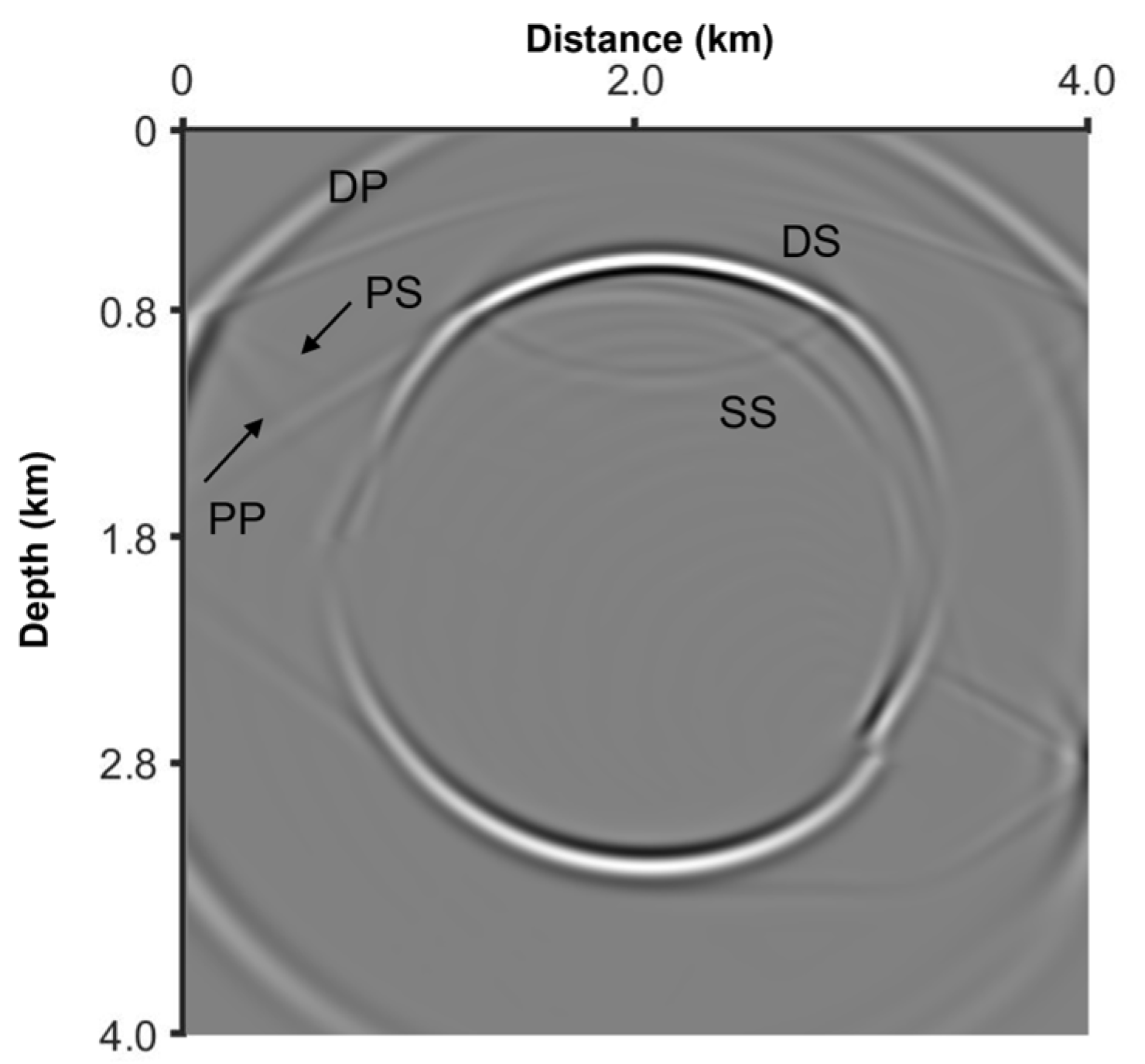
3.1. Homogeneous Model

We first investigate the accuracy and efficiency of the proposed ALHSGGL method with different stencil lengths. The P- and S-wave velocities are 2500 and 1443 m/s, respectively, and the density is 2200 kg/m³. We have considered Q_P = 32 and Q_S= 16. The model is discretized in a mesh with $500\times 500$ grid points using a 10 m grid spacing in both the horizontal and vertical directions, and the time step is 1.0 ms. The source (a vertical force) has a Ricker ($s\left(t\right)=-5.76f_0^2\left[1-16{\left(0.6f_{0}t-1\right)}^2\right]e^{-8{\left(0.6f_{0}t-1\right)}^2}$) time history with a 25 Hz center frequency and is located at (250, 250) points. Figure 1 compares the seismograms recorded at (370, 250) point between the ALHSGGL method $N_{\epsilon ,\gamma }=$44, 15, 5, 3 (the coarse grid $\Delta x=\Delta z=10 \mathrm{m}$) and the reference solutions (the fine grid $\Delta x=\Delta z=4 \mathrm{m}$). We observe that the numerical solutions (blue dash) almost overlap with the reference solution (red line). Although the relative error (black dot) shows a slight bias at $\epsilon <{10}^{-2}$, the overall performance is satisfactory, with the maximum total error not exceeding 0.17%. Furthermore, when computing the fractional partial derivative at a single grid point, the GSGGL method requires 9000 floating-point operations. In comparison, the ALHSGGL method requires 797, 259, 95, and 59 floating-point operations, respectively. The computational time for simulating the lengths of these four differential operators constitutes only 4.67%, 4.47%, 4.44%, and 4.42% of the total time required by the conventional differential methods.

To investigate the effects of dispersion and attenuation in viscoelastic media, we separately present the behavior of the wavefield amplitude loss and phase distortion. Figure 2 shows a snapshot that encompasses various wave propagation properties, including the elastic (lossless), loss-dominated, dispersion-dominated, and viscoelastic (lossy) characteristics. The distinct characteristics are separated using a dashed line. The P-wavefront is depicted by a red line, while the S-wavefront is represented by a blue line. Compared with the elastic wavefield (Figure 2a), Figure 2b,d have a phase delay because the highly viscous media tends to resist the wave propagation. Figure 2c,d exhibit amplitude loss, while the Figure 2c amplitude loss remains unchanged in terms of travel time. When both the dispersion and attenuation effects are considered (Figure 2d), the simulated viscoelastic wavefield contains both amplitude loss and phase distortion.

3.2. Fault Model

This model is designed to assess the algorithm’s adaptability to sharp contrasts in the P-wave velocity and Q_P. As shown in Figure 3, the central area of the model features a sharp interface. The Q_P-value is set using an empirical formula $Q=3.516\times v^{2.2}$ [41,42]. It is discretized with $400\times 400$ grid points and spacings of 10 m. The source is located at (1.8, 2.0) km with 25 Hz. The time step is 1 ms, and convolutional perfectly matched layer (CPML) [43] absorbing strips, with a width of 30 grid points, are implemented at the four boundaries of the computational mesh to avoid wraparound. Figure 4 shows the viscoelastic vertical-component snapshots at 0.7 s. The snapshots clearly show the direct P- and S-waves, the reflected PP and PS waves, and other waveforms. The simulated wavefields in Figure 4 are stable, indicating that the ALHSGGL scheme can be used to simulate the wavefield stably in arbitrary complex media.

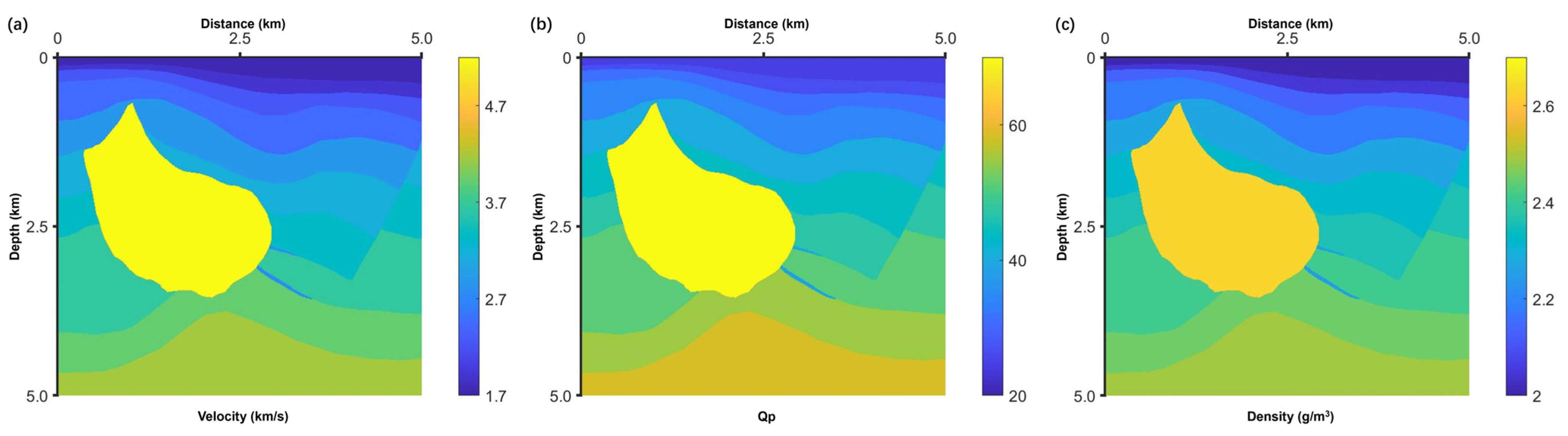
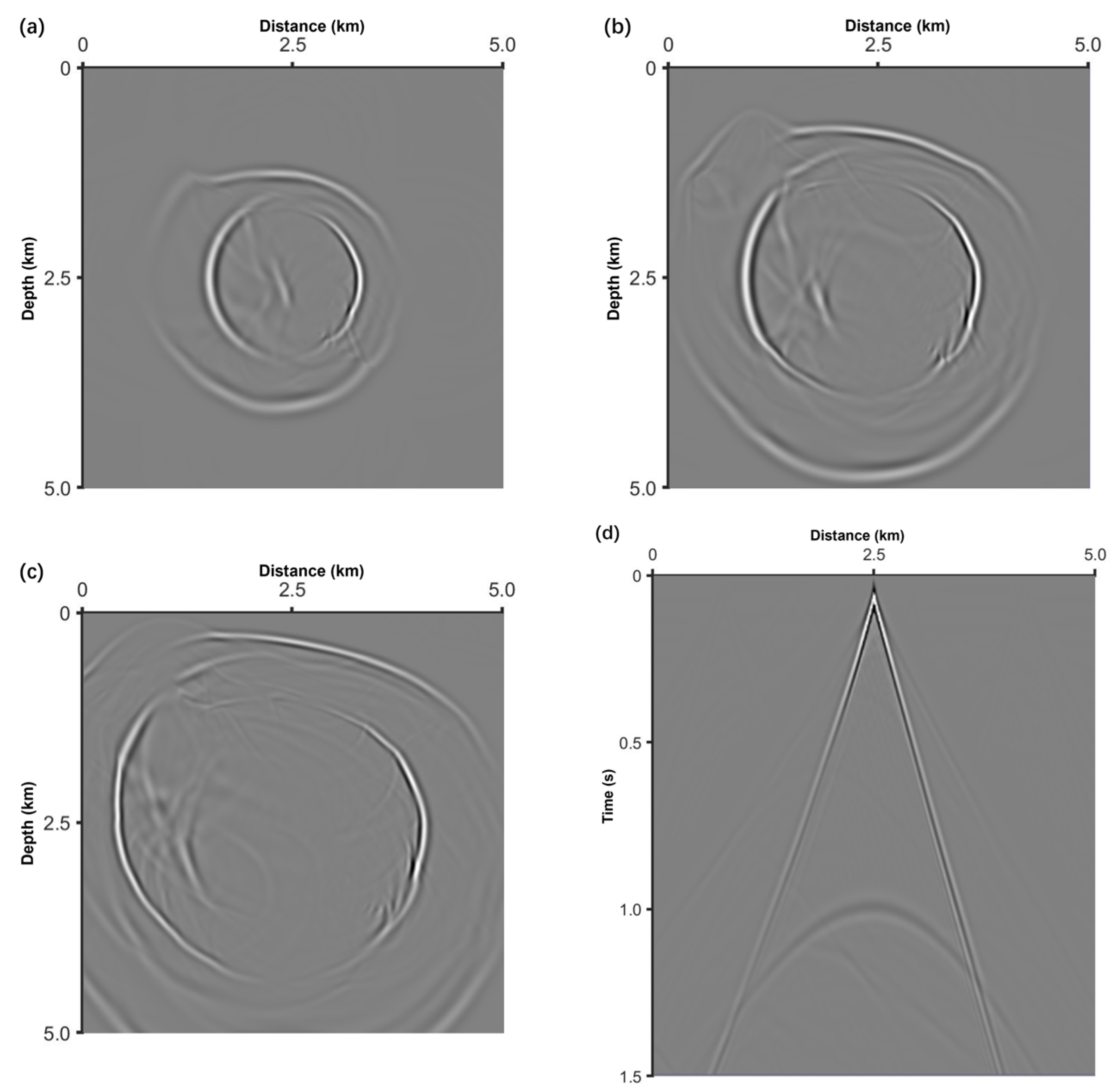
3.3. Hess Salt Model

We test the algorithm on the Hess salt model, which includes velocity anomalies in the middle of the region. The P-wave velocity ranges from 1.753 to 5.189 km/s; the Q_P-value and the density are shown in Figure 5a–c. The computational domain is 0 km to 5 km in both the horizontal and vertical directions using a 10 m grid spacing. The time step is 1 ms. The Ricker wavelet source, with a 25 Hz center frequency, is placed at (2.5, 2.5) km. Figure 6a–c show the wavefield snapshots at 0.4 s, 0.6 s, and 0.8 s, respectively.

It can be observed that when the wave propagates through the low-velocity and high-attenuation zone, both the waveform and energy undergo significant changes. As the wave propagates to the bottom area, the direct wave is muted. The presence of gas chimneys in shallow strata can strongly attenuate the energy of seismic compression waves, which is observable in the seismograms at 6.0 s, as shown in Figure 6d. This indicates that the ALHSGGL method can stably simulate the wavefield in arbitrarily complex media.

4. Conclusions

In the current paper, we develop an effective forward simulation method for simulating fractional viscoelastic seismic wavefields. To achieve this, we use the arbitrary-order SG method to approximate the first-order velocity–stress terms and apply the GL finite difference approximation to the fractional-order operator. The resulting hybrid discretization scheme can be directly applied to solve the viscoelastic wave equation in the time-spatial domain, thus avoiding the FFT and IFFT operations required at each time step in the traditional Fourier-based methods, while offering enhanced programmability. The truncation error and stability analysis provided indicate that the proposed method can perform calculations stably and accurately at the exploration scale. Next, we present a stencil index for compact difference operators for the convenience of the reader. Numerical simulations of the fault model and the Hess salt model demonstrate the accurate propagation capabilities of the HSGGL method in heterogeneous attenuating media, making it an excellent forward engine for RTM and FWI techniques. We anticipate that the proposed method could provide valuable references for simulating heterogeneous media.

References

1. McDonal, F.; Angona, F.; Mills, R.; Sengbush, R.; Van Nostrand, R.; White, J. Attenuation of shear and compressional waves in Pierre shale. Geophysics 1958, 23, 421–439. [Google Scholar] [CrossRef]
2. Carcione, J.M.; Santos, J.E.; Picotti, S. Fracture-induced anisotropic attenuation. Rock Mech. Rock Eng. 2012, 45, 929–942. [Google Scholar] [CrossRef]
3. Wang, Y.; Ning, Y.; Wang, Y. Fractional Time Derivative Seismic Wave Equation Modeling for Natural Gas Hydrate. Energies 2020, 13, 5901. [Google Scholar] [CrossRef]
4. Li, Q.; Fu, L.Y.; Zhou, H.; Wei, W.; Hou, W. Effective Q-compensated reverse time migration using new decoupled fractional Laplacian viscoacoustic wave equation. Geophysics 2018, 84, 57–69. [Google Scholar] [CrossRef]
5. Sun, J.; Zhu, T. Strategies for stable attenuation compensation in reverse-time migration. Geophys. Prospect. 2018, 66, 498–511. [Google Scholar] [CrossRef]
6. Chen, H.; Zhou, H.; Rao, Y. An implicit stabilization strategy for Q-compensated reverse time migration. Geophysics 2020, 85, S169–S183. [Google Scholar] [CrossRef]
7. Mu, X.; Huang, J. A simple and high-efficient viscoacoustic reverse time migration calculated by finite difference. Geophysics 2023, 88, S213–S223. [Google Scholar] [CrossRef]
8. Li, J.; Yang, D.; Wang, Z.; Liu, L. Attenuation-compensated reverse time migration based on the stereo-modeling operator. Geophysics 2023, 88, S175–S187. [Google Scholar] [CrossRef]
9. Chen, H.; Zhou, H.; Rao, Y. Source wavefield reconstruction in fractional Laplacian viscoacoustic wave equation-based full waveform inversion. IEEE Trans. Geosci. Remote Sens. 2020, 59, 6496–6509. [Google Scholar] [CrossRef]
10. Xing, G.; Zhu, T. Decoupled Fréchet kernels based on a fractional viscoacoustic wave equation. Geophysics 2022, 87, T61–T70. [Google Scholar] [CrossRef]
11. Hu, B.T.; Huang, C.; Dong, L.G.; Zhang, J.M. A constant fractional Laplacian operator based viscoacoustic full waveform inversion for velocity and attenuation estimation. Chin. J. Geophys. 2023, 66, 2123–2137. [Google Scholar]
12. Bai, T.; Tsvankin, I. Time-domain finite-difference modeling for attenuative anisotropic media. Geophysics 2016, 81, C69–C77. [Google Scholar] [CrossRef]
13. Kjartansson, E. Constant-Q wave propagation and attenuation. J. Geophys. Res. 1979, 84, 4737–4748. [Google Scholar] [CrossRef]
14. Carcione, J.M.; Kosloff, D.; Kosloff, R. Wave propagation simulation in a linear viscoacoustic medium. Geophys. J. Int. 1988, 95, 597–611. [Google Scholar] [CrossRef]
15. Carcione, J.M. A generalization of the Fourier pseudospectral method. Geophysics 2010, 75, A53–A56. [Google Scholar] [CrossRef]
16. Zhu, T.; Carcione, J.M.; Harris, J.M. Approximating constant-Q seismic propagation in the time domain. Geophys. Prospect. 2013, 61, 931–940. [Google Scholar] [CrossRef]
17. Zhang, Y.; Chen, T.; Zhu, H.; Liu, Y.; Xing, T.; Zhang, X. Approximating constant-Q seismic wave propagations in acoustic and elastic media using a Cole–Cole model. Bull. Seismol. Soc. Am. 2023, 113, 312–332. [Google Scholar] [CrossRef]
18. Zhu, T.; Harris, J.M. Modeling acoustic wave propagation in heterogeneous attenuating media using decoupled fractional Laplacians. Geophysics 2014, 79, T105–T116. [Google Scholar] [CrossRef]
19. Xing, G.; Zhu, T. Modeling frequency-independent Q viscoacoustic wave propagation in heterogeneous media. J. Geophys. Res. Solid Earth 2019, 112, 11568–11584. [Google Scholar] [CrossRef]
20. Mu, X.; Huang, J.; Wen, L.; Zhuang, S. Modeling viscoacoustic wave propagation using a new spatial variable-order fractional Laplacian wave equation. Geophysics 2021, 86, T487–T507. [Google Scholar] [CrossRef]
21. Zhang, Y.; Zhu, H.; Liu, Y.; Chen, T. Power-law frequency-dependent Q simulations in viscoacoustic media using decoupled fractional Laplacians. Geophysics 2024, 89, T183–T194. [Google Scholar] [CrossRef]
22. Zhu, T.; Carcione, J.M. Theory and modelling of constant-Q P- and S-waves using fractional spatial derivatives. Geophys. J. Int. 2014, 196, 1787–1795. [Google Scholar] [CrossRef]
23. Mu, X.; Huang, J.; Yang, J.; Li, Z.; Ivan, M.S. Viscoelastic wave propagation simulation using new spatial variable-order fractional Laplacians. Bull. Seismol. Soc. Am. 2022, 112, 48–77. [Google Scholar] [CrossRef]
24. Zhang, Y.; Liu, Y.; Zhu, H.; Chen, T.; Li, J. Modified viscoelastic wavefield simulations in the time domain using the new fractional Laplacians. J. Geophys. Eng. 2022, 19, 346–361. [Google Scholar] [CrossRef]
25. Han, G.; He, B.; Zhang, H.; Wang, E. Fractional-order velocity-dilatation-rotation viscoelastic wave equation and numerical solution based on a constant-Q model. Geophysics 2024, 89, T111–T123. [Google Scholar] [CrossRef]
26. Carcione, J.; Cavallini, F.; Mainardi, F. Time-domain seismic modeling of constant Q-wave propagation using fractional derivatives. Pure Appl. Geophys. 2002, 159, 1719–1736. [Google Scholar] [CrossRef]
27. Carcione, J.M. Theory and modeling of constant-Q P- and S waves using fractional time derivatives. Geophysics 2009, 74, T1–T11. [Google Scholar] [CrossRef]
28. Zhu, T. Numerical simulation of seismic wave propagation in viscoelastic-anisotropic media using frequency-independent Q wave equation. Geophysics 2017, 82, WA1–WA10. [Google Scholar] [CrossRef]
29. Carcione, J.M.; Picotti, S.; Ba, J. P- and S-wave simulation using a Cole-Cole model to incorporate thermoelastic attenuation and dispersion. J. Acoust. Soc. Am. 2021, 149, 1946–1954. [Google Scholar] [CrossRef]
30. Chen, W.; Holm, S. Fractional Laplacian time-space models for linear and nonlinear lossy media exhibiting arbitrary frequency power-law dependency. J. Acoust. Soc. Am. 2004, 115, 1424–1430. [Google Scholar] [CrossRef] [PubMed]
31. Treeby, B.E.; Cox, B.T. Modeling power law absorption and dispersion for acoustic propagation using the fractional Laplacian. J. Acoust. Soc. Am. 2010, 127, 2741–2748. [Google Scholar] [CrossRef]
32. Sun, J.; Zhu, T.; Fomel, S. Viscoacoustic modeling and imaging using low-rank approximation. Geophysics 2015, 80, A103–A108. [Google Scholar] [CrossRef]
33. Chen, H.; Zhou, H.; Li, Q.; Wang, Y. Two efficient modeling schemes for fractional Laplacian viscoacoustic wave equation. Geophysics 2016, 81, T233–T249. [Google Scholar] [CrossRef]
34. Wang, N.; Xing, G.; Zhu, T. Accurately propagating P- and S-waves in attenuation media using spatial-independent-order decoupled fractional Laplacians. In SEG Technical Program Expanded Abstracts; Society of Exploration Geophysicists: Houston, TX, USA, 2019; pp. 3805–3809. [Google Scholar]
35. Xue, Z.; Baek, H.; Zhang, H.; Zhao, Y.; Zhu, T.; Fomel, S. Solving fractional Laplacian viscoelastic wave equations using domain decomposition. In Proceedings of the 2018 SEG International Exposition and Annual Meeting, Anaheim, CA, USA, 14–19 October 2018; pp. 3943–3947. [Google Scholar]
36. Gu, B.; Zhang, S.; Liu, X.; Han, J. Efficient modeling of fractional Laplacian viscoacoustic wave equation with fractional finite-difference method. Comput. Geosci. 2024, 191, 0098–3004. [Google Scholar] [CrossRef]
37. Yao, J.; Zhu, T.; Hussain, F.; Kouri, D.J. Locally solving fractional Laplacian viscoacoustic wave equation using Hermite distributed approximating functional method. Geophysics 2017, 82, T59–T67. [Google Scholar] [CrossRef]
38. Ji, M.; Kouri, D.; Zhu, T.; Yao, J. Using PSPI to accelerate seismic Q modeling based on Hermite-distributed approximating functional. In Proceedings of the 2017 SEG International Exposition and Annual Meeting, Houston, TX, USA, 27 September 2017; pp. 4091–4096. [Google Scholar]
39. Song, G.; Zhang, X.; Wang, Z.; Chen, Y.; Chen, P. The asymptotic local finite difference method of the fractional wave equation and its viscous seismic wavefield simulation. Geophysics 2020, 85, T179–T189. [Google Scholar] [CrossRef]
40. Moczo, P.; Kristek, J.; Halada, L. 3D Fourth-order staggered grid finite-difference schemes: Stability and grid dispersion. Bull. Seismol. Soc. Am. 2000, 90, 587–603. [Google Scholar] [CrossRef]
41. Li, Q. High Resolution Seismic Data Processing; Petroleum Industry Press: Beijing, China, 1993. [Google Scholar]
42. Yan, H.; Liu, Y. Visco-acoustic prestack reverse-time migration based on the time-space domain adaptive high-order finite-difference method. Geophys. Prospect. 2013, 61, 941–954. [Google Scholar] [CrossRef]
43. Komatitsch, D.; Martin, R. An unsplit convolutional perfectly matched layer improved at grazing incidence for the seismic wave equation. Geophysics 2007, 72, SM155–SM167. [Google Scholar] [CrossRef]
Figure 1. Comparison between numerical solutions (blue dash) and reference solution (red line) generated by ALHSGGL method as well as their residuals (black dot) in the homogeneous model for (a) ε = 10 5 , (b) ε = 10 4 , (c) ε = 10 3 , and (d) ε = 10 2 .
Fractalfract 09 00153 g001
Figure 2. Wavefield snapshots simulated using elastic, dissipation-dominated, dispersive-dominated, and viscoelastic wave equations. Dashed red lines represent P-wavefront, and solid blue lines represent S-wavefront.
Fractalfract 09 00153 g002
Figure 3. Fault model with properties. A 25 Hz dominant frequency Ricker wavelet is chosen as a vertical force and located at (1.8, 2.0) km.
Fractalfract 09 00153 g003
Figure 4. Wavefield snapshots of fault model at 0.7 s. Symbols denote as follows: DP: direct P-wave; DS: direct S-wave; PP: reflected P-waves at second interface; PS: converted S-waves from P-waves at second interface; SS: reflected S-waves.
Fractalfract 09 00153 g004
Figure 5. The Hess salt model: (a) The P-wave velocity, (b) the QP parameters, and (c) the density parameters for the Hess model. The S-wave velocity and QS parameters are constructed by the relations V S = V P / 3 and Q S = Q P / 1.2 , respectively.
Fractalfract 09 00153 g005
Figure 6. Wavefield snapshots of Hess salt model at (a) 0.4 s, (b) 0.6 s, (c) 0.8 s, and (d) surface seismograms at 6.0 s.
Fractalfract 09 00153 g006