
Analysis Modulation Instability and Parametric Effect on Soliton Solutions for M-Fractional Landau–Ginzburg–Higgs (LGH) Equation Through Two Analytic Methods


Abstract
1. Introduction
2. Fractional Derivative
- i.
- .
- ii.
- .
- iii.
- .
- iv.
- ; here, is an arbitrary constant.
- v.
- .
3. Analytical Method
3.1. Modified F-Expansion Method
- If .
- If .
- If .
- If .
- If .
- If .
- If .
- If .
- If .
- If .
- If .
- If .
3.2. Newly Improved Kudryashov’s Method
4. Soliton Solutions of M-Fractional Landau–Ginzburg–Higgs Equation
4.1. Application of the Modified F-Expansion Method
4.2. Application of the Newly Improved Kudryashov’s Method
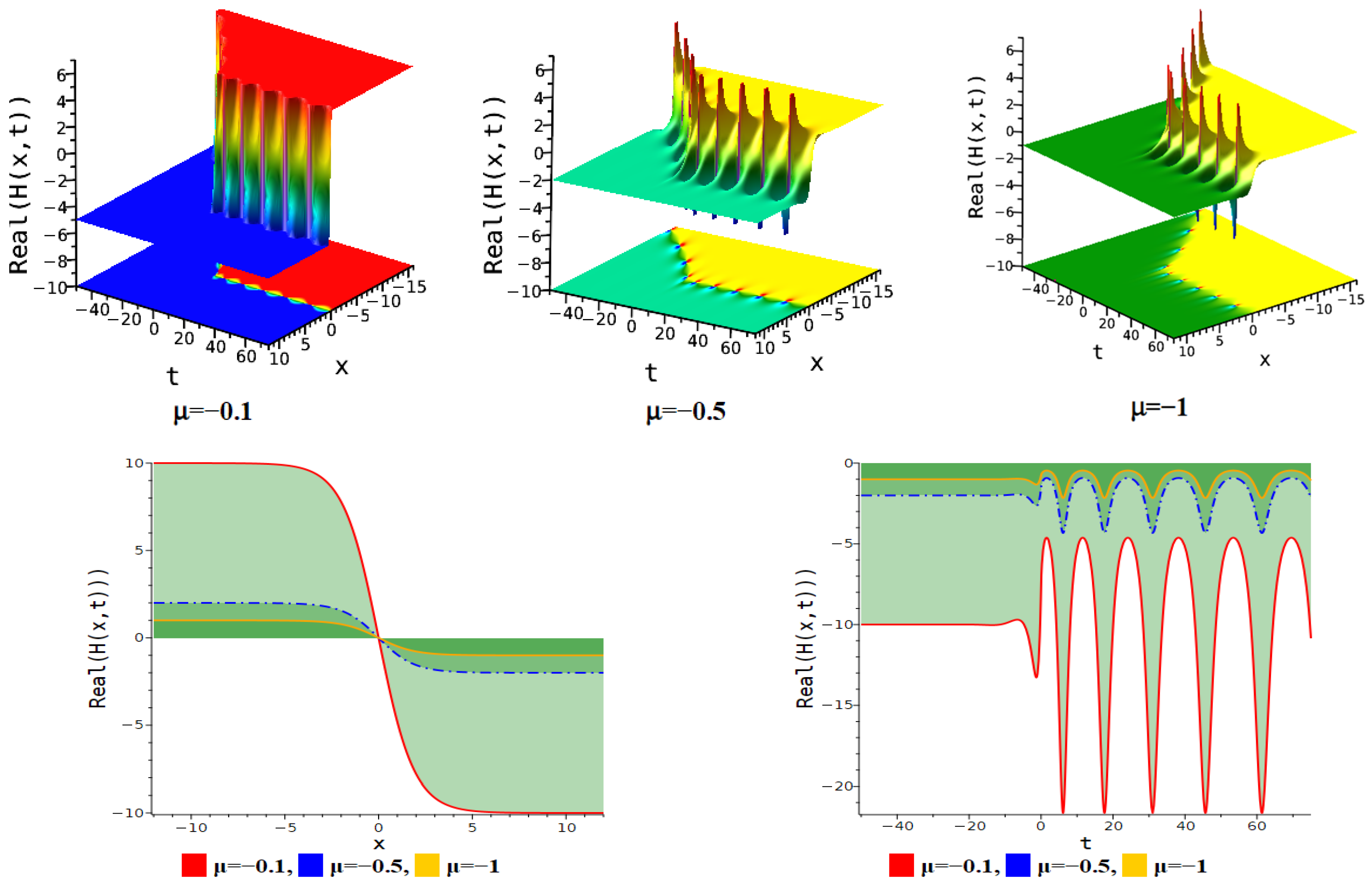
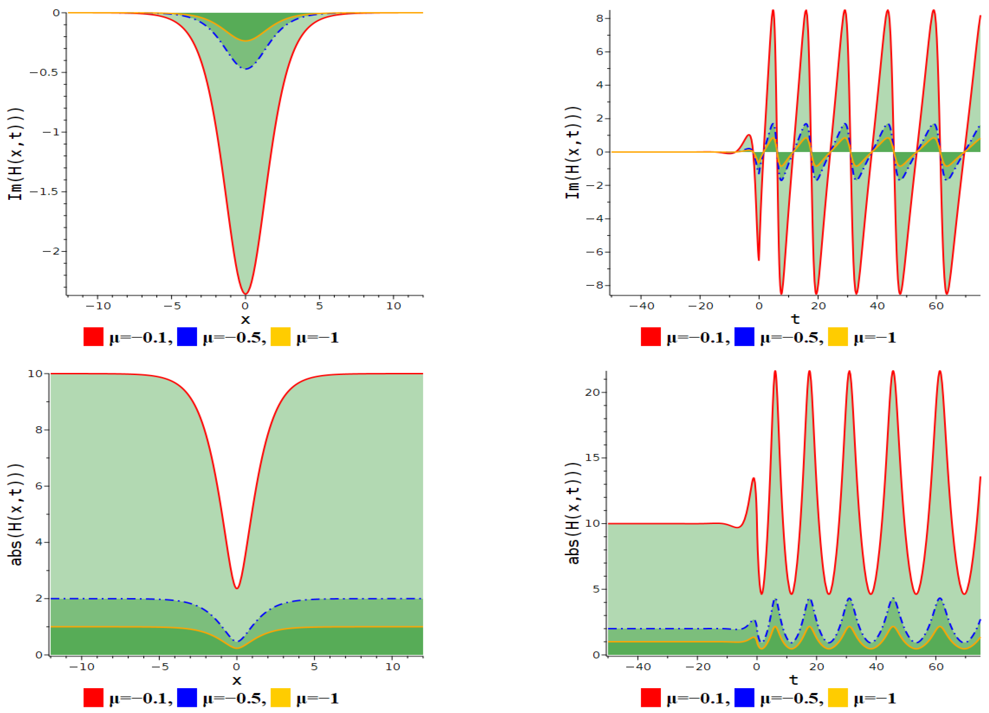
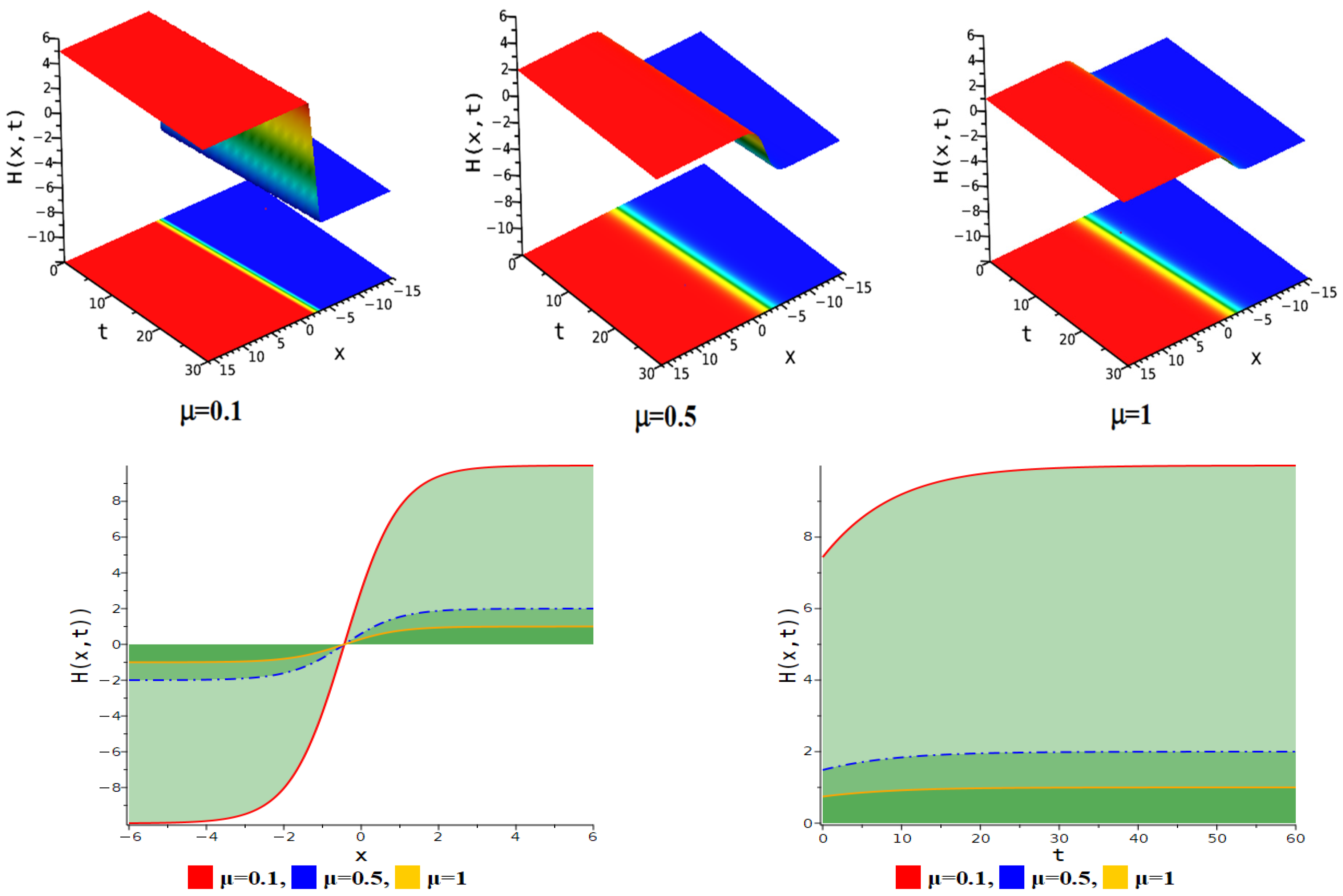
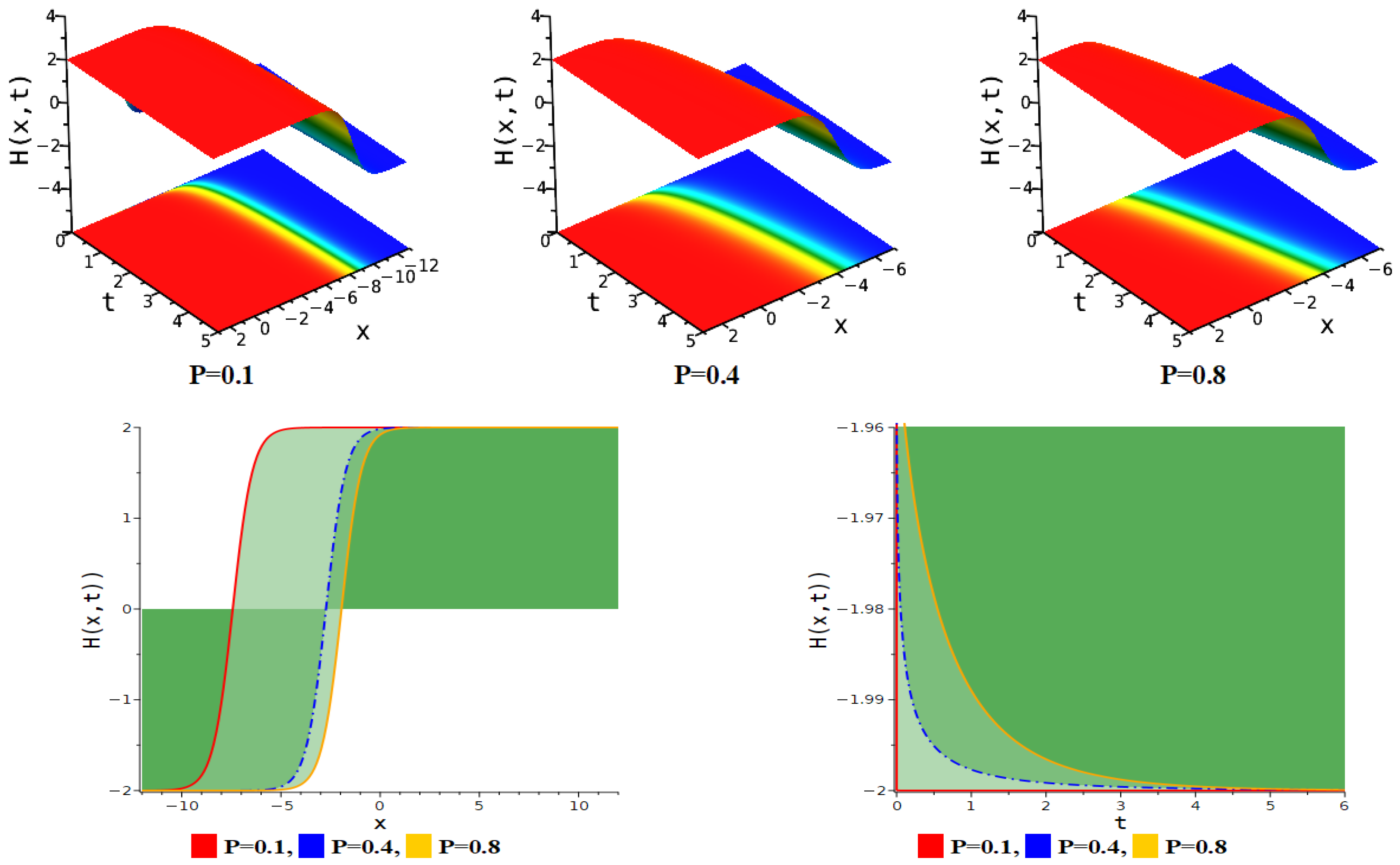
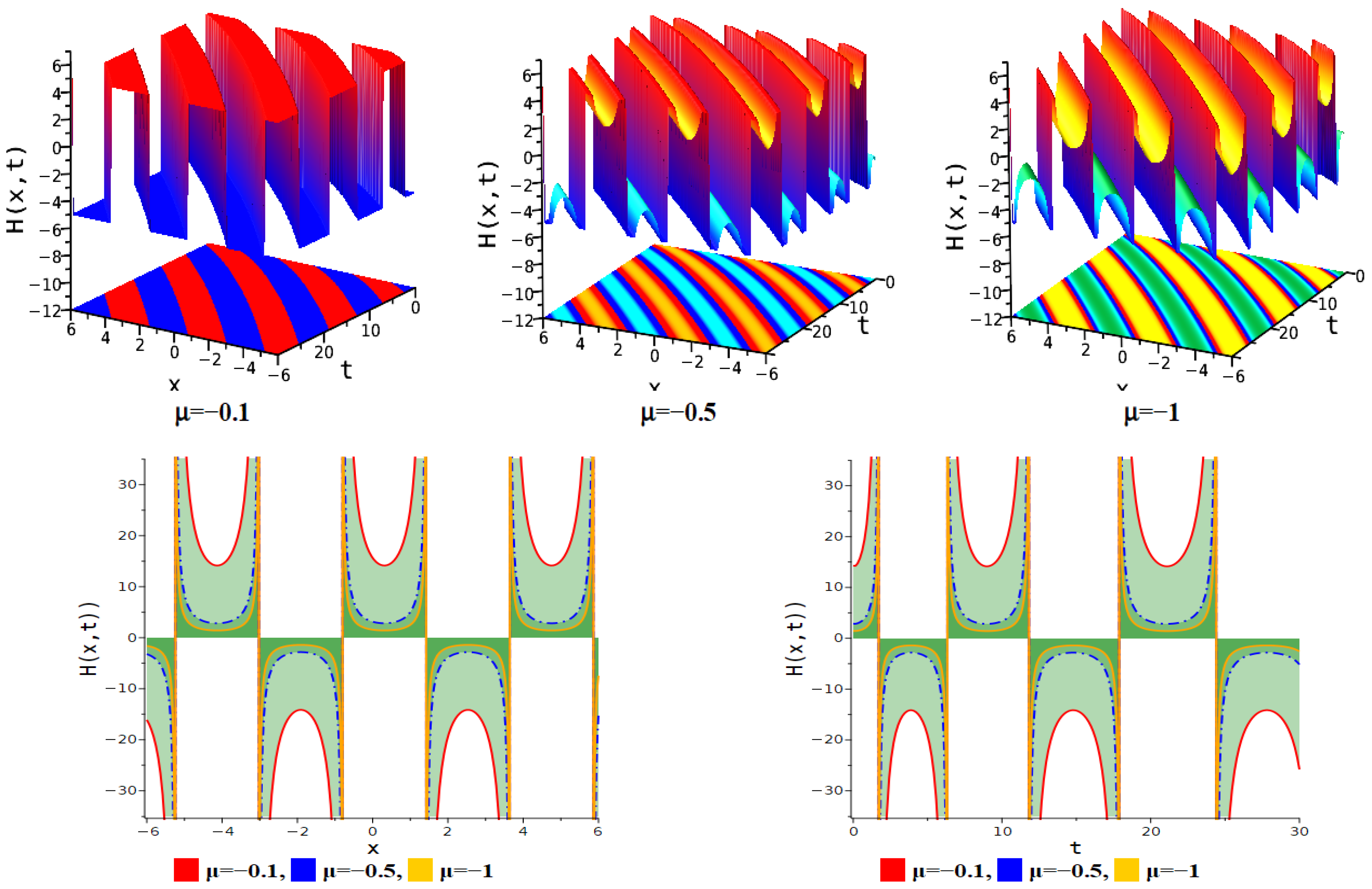
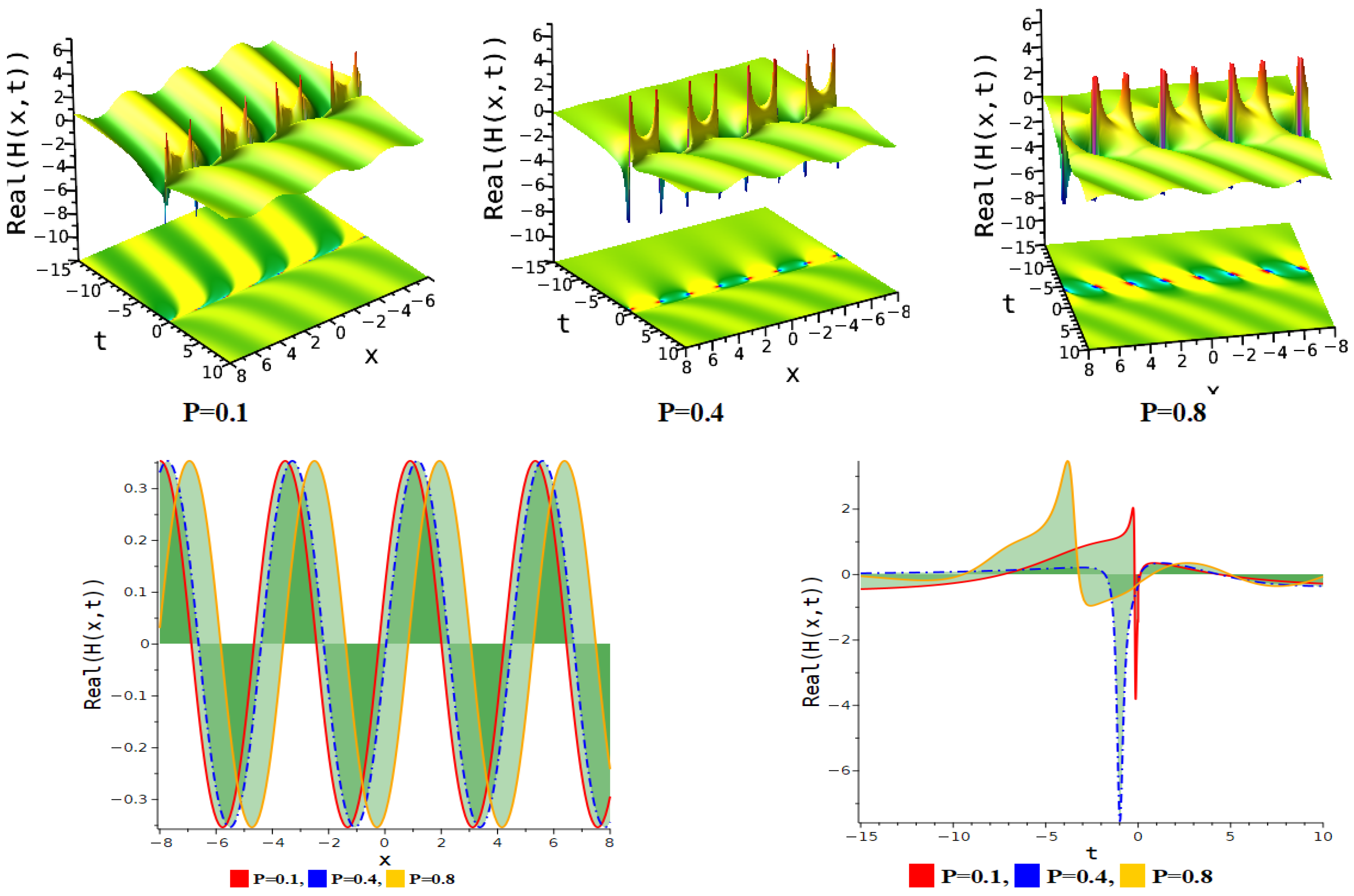
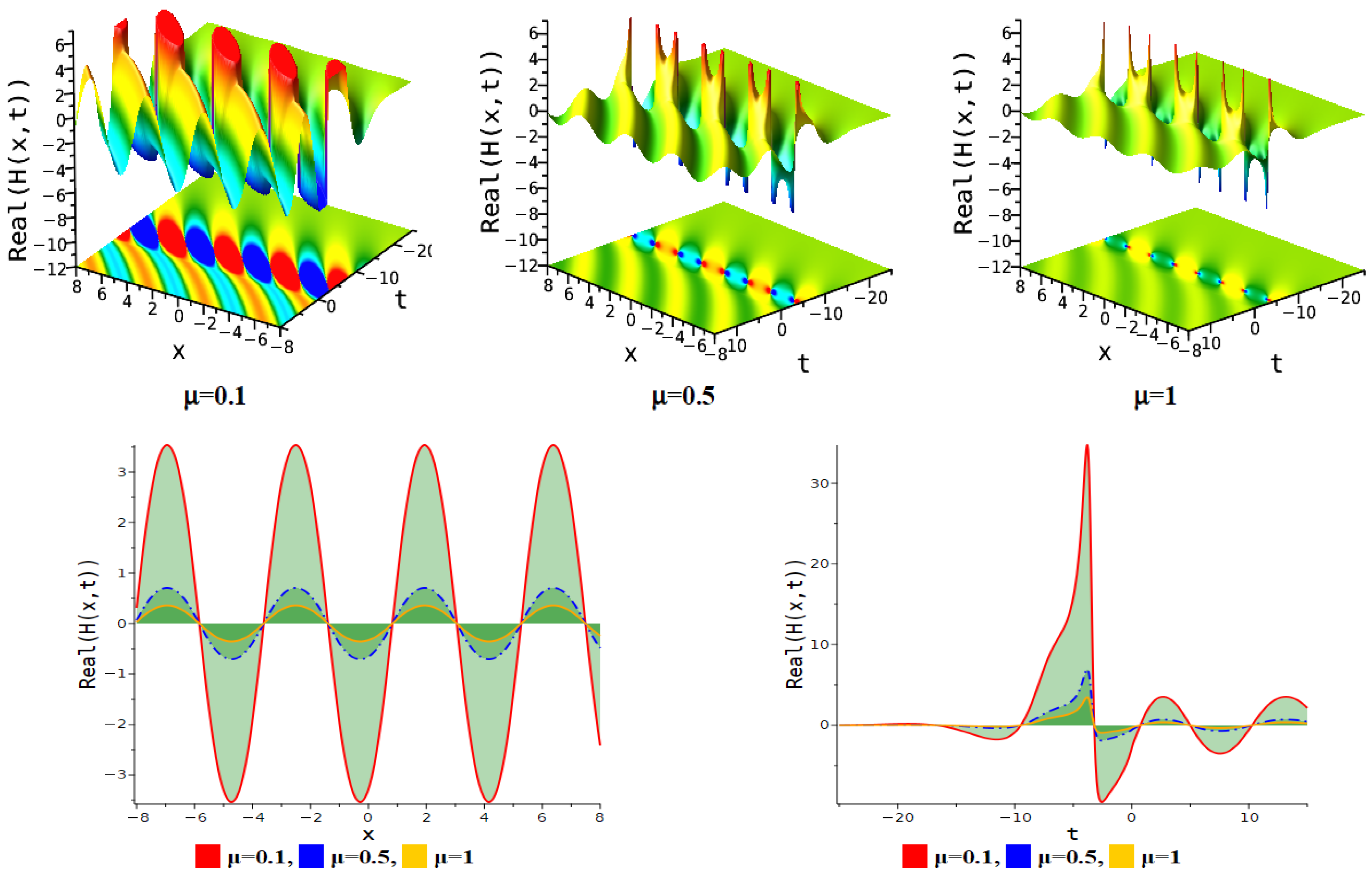
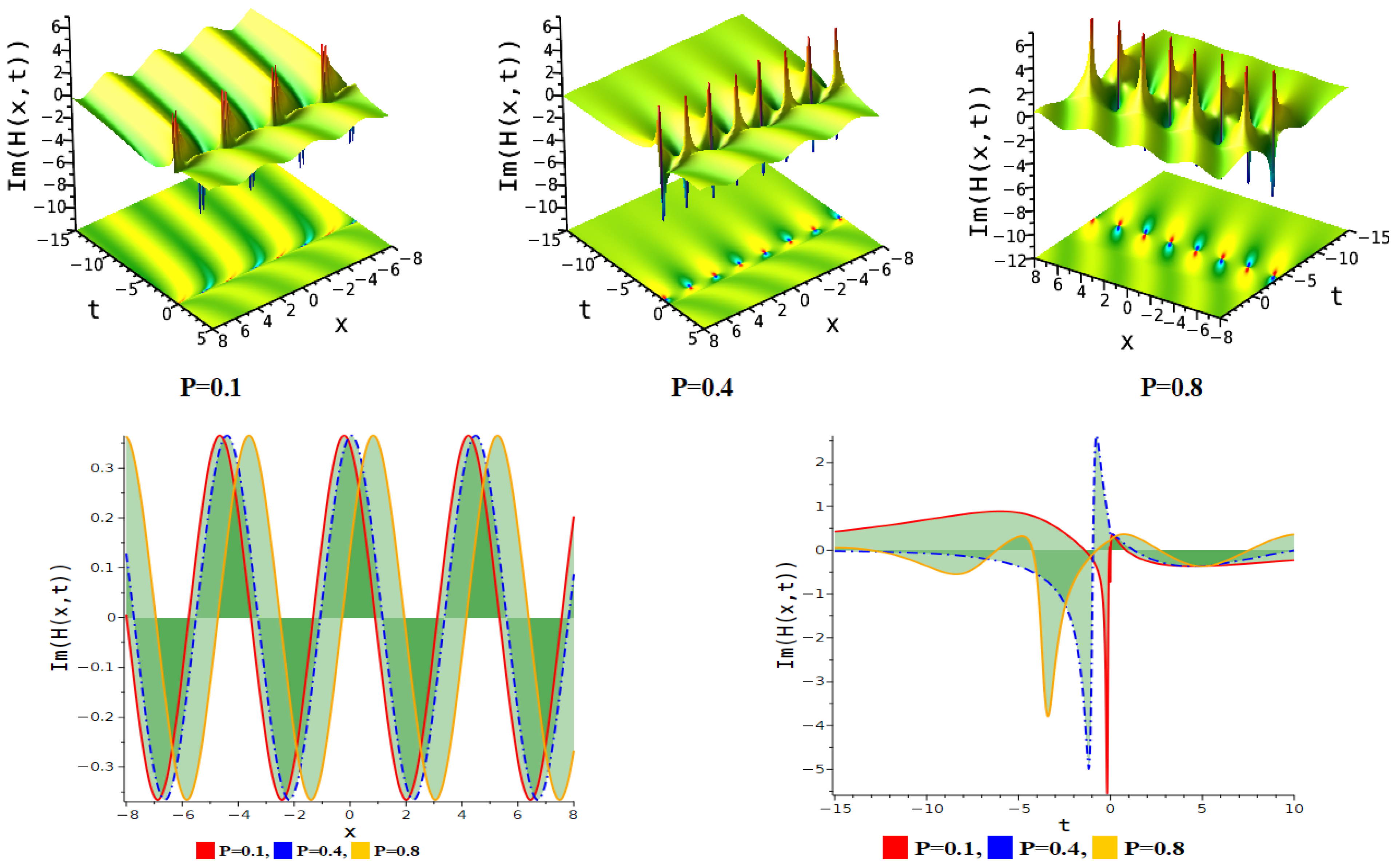
5. Figure Analysis
5.1. Figure Analysis of the Modified F-Expansion Method
5.2. Figure Analysis of the Newly Improved Kudryashov’s Method
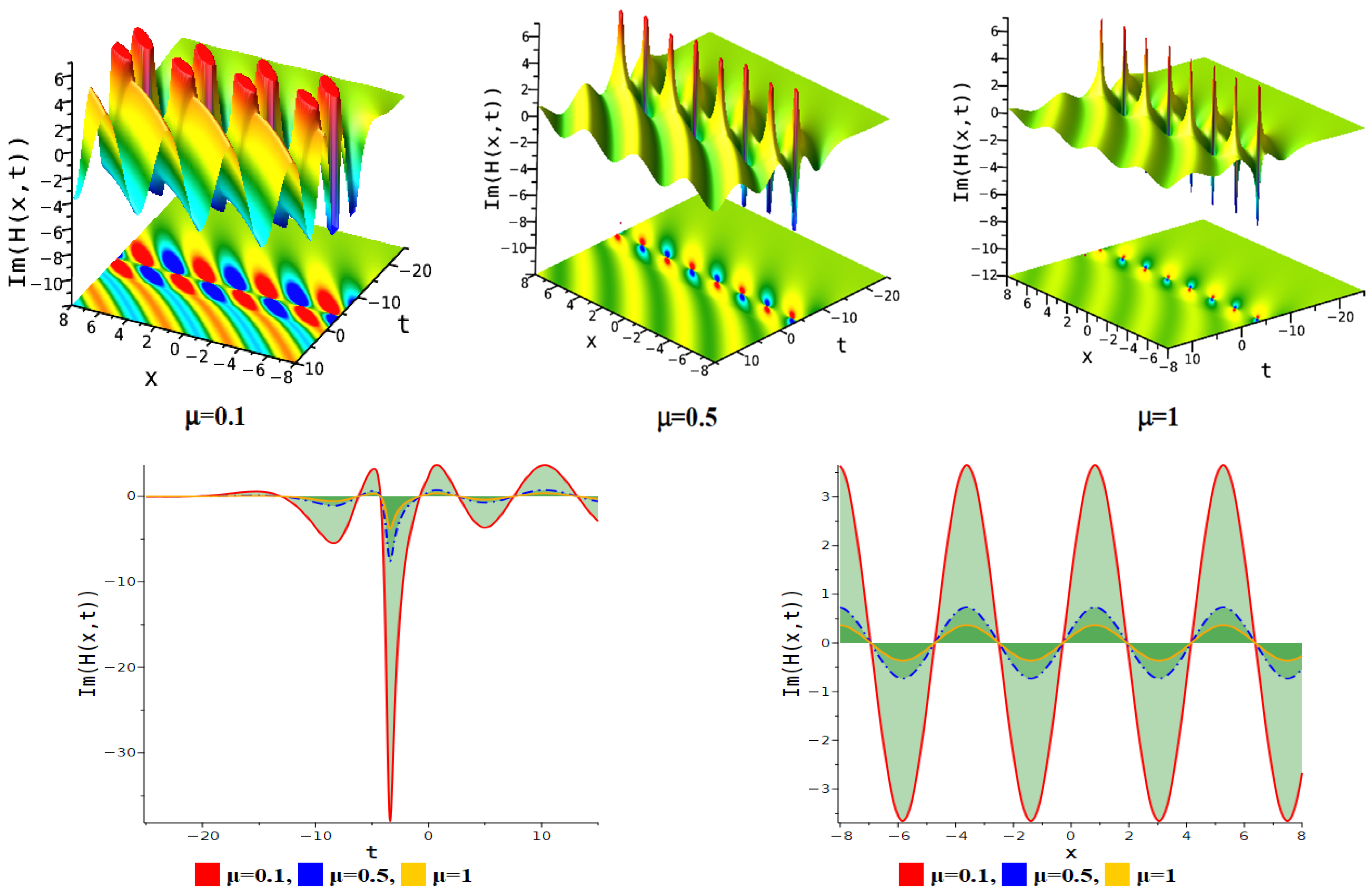
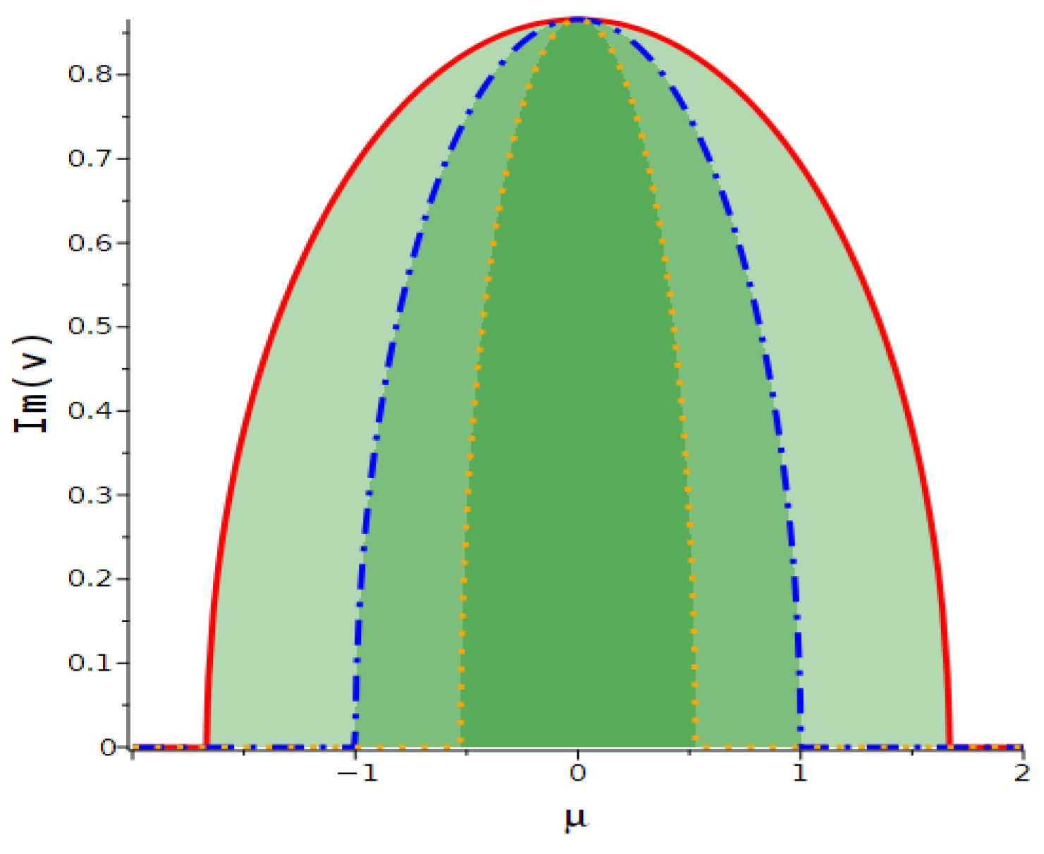
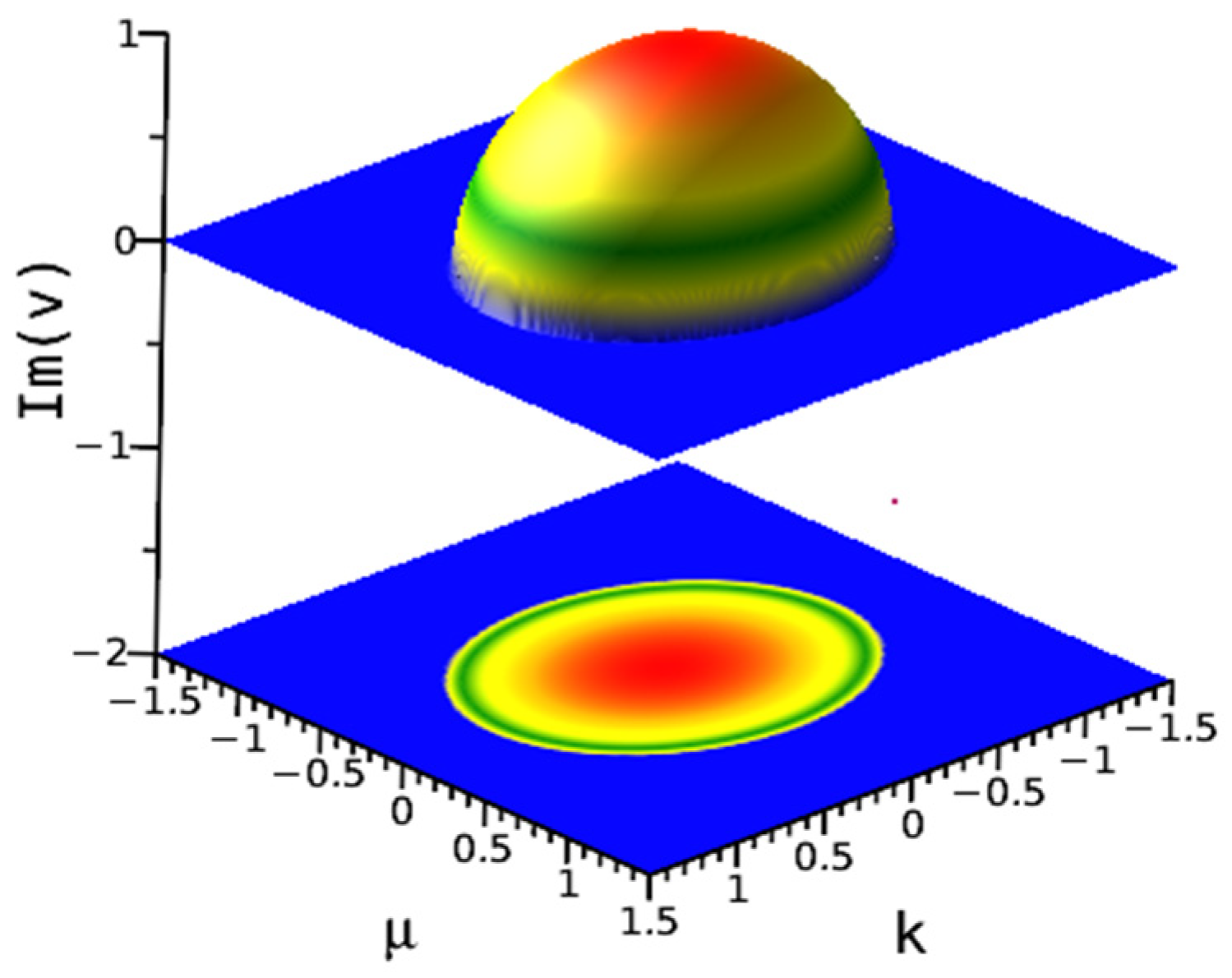
6. Modulation Instability
7. Comparison and Novelty of This Work
7.1. Comparison with the Existing Works
7.2. Novelty of This Work
8. Conclusions
Author Contributions
Funding
Data Availability Statement
Acknowledgments
Conflicts of Interest
References
- Madhukalya, B.; Kalita, J.; Das, R.; Hosseini, K.; Baleanu, D.; Osman, M.S. Dynamics of Ion-Acoustic Solitary Waves in Three-Dimensional Magnetized Plasma with Thermal Ions and Electrons: A Pseudopotential Analysis. Opt. Quantum Electron. 2024, 56, 898. [Google Scholar] [CrossRef]
- Faridi, W.A.; Iqbal, M.; Ramzan, B.; AlQahtani, S.A.; Osman, M.S.; Akinyemi, L.; Mostafa, A.M. The Formation of Invariant Optical Soliton Structures to Electric-Signal in the Telegraph Lines on Basis of the Tunnel Diode and Chaos Visualization, Conserved Quantities: Lie Point Symmetry Approach. Optik 2024, 305, 171785. [Google Scholar] [CrossRef]
- Madhukalya, B.; Das, R.; Hosseini, K.; Hincal, E.; Osman, M.S.; Wazwaz, A.M. Nonlinear Analysis of Ion-acoustic Solitary Waves in an Unmagnetized Highly Relativistic Quantum Plasma. Heat Trans. 2024, 53, 4036–4051. [Google Scholar] [CrossRef]
- Zhang, Z.; Huang, J.; Zhong, J.; Dou, S.-S.; Liu, J.; Peng, D.; Gao, T. The Extended (G′/G)-Expansion Method and Travelling Wave Solutions for the Perturbed Nonlinear Schrödinger’s Equation with Kerr Law Nonlinearity. Pramana-J. Phys. 2014, 82, 1011–1029. [Google Scholar] [CrossRef]
- Adel, M.; Aldwoah, K.; Alharbi, F.; Osman, M.S. Dynamic Properties of Non-Autonomous Femtosecond Waves Modeled by the Generalized Derivative NLSE with Variable Coefficients. Crystals 2022, 12, 1627. [Google Scholar] [CrossRef]
- Saber, H.; Alqarni, F.A.; Aldwoah, K.A.; Hashim, H.E.; Saifullah, S.; Hleili, M. Novel Hybrid Waves Solutions of Sawada–Kotera like Integrable Model Arising in Fluid Mechanics. Alex. Eng. J. 2024, 104, 723–744. [Google Scholar] [CrossRef]
- Ozisik, M.; Onder, I.; Esen, H.; Cinar, M.; Ozdemir, N.; Secer, A.; Bayram, M. On the Investigation of Optical Soliton Solutions of Cubic–Quartic Fokas–Lenells and Schrödinger–Hirota Equations. Optik 2023, 272, 170389. [Google Scholar] [CrossRef]
- Kumar, S.; Mann, N.; Kharbanda, H.; Inc, M. Dynamical Behavior of Analytical Soliton Solutions, Bifurcation Analysis, and Quasi-Periodic Solution to the (2+1)-Dimensional Konopelchenko–Dubrovsky (KD) System. Anal. Math. Phys. 2023, 13, 40. [Google Scholar] [CrossRef]
- Sabi’u, J.; Sirisubtawee, S.; Inc, M. Optical Soliton Solutions for the Chavy-Waddy-Kolokolnikov Model for Bacterial Colonies Using Two Improved Methods. J. Appl. Math. Comput. 2024, 70, 5459–5482. [Google Scholar] [CrossRef]
- Khater, M.M.A. Analytical Simulations of the Fokas System; Extension (2+1)-Dimensional Nonlinear Schrödinger Equation. Int. J. Mod. Phys. B 2021, 35, 2150286. [Google Scholar] [CrossRef]
- Hossen, M.B.; Roshid, H.O.; Ali, M.Z. Dynamical Structures of Exact Soliton Solutions to Burgers’ Equation via the Bilinear Approach. Partial. Differ. Equ. Appl. Math. 2021, 3, 100035. [Google Scholar] [CrossRef]
- Mahmood, A.; Srivastava, H.M.; Abbas, M.; Abdullah, F.A.; Mohammed, P.O.; Baleanu, D.; Chorfi, N. Optical Soliton Solutions of the Coupled Radhakrishnan-Kundu-Lakshmanan Equation by Using the Extended Direct Algebraic Approach. Heliyon 2023, 9, e20852. [Google Scholar] [CrossRef] [PubMed]
- Muniyappan, A.; Manikandan, K.; Saparbekova, A.; Serikbayev, N. Exploring the Dynamics of Dark and Singular Solitons in Optical Fibers Using Extended Rational Sinh–Cosh and Sine–Cosine Methods. Symmetry 2024, 16, 561. [Google Scholar] [CrossRef]
- Yokus, A.; Durur, H.; Ahmad, H.; Thounthong, P.; Zhang, Y.-F. Construction of Exact Traveling Wave Solutions of the Bogoyavlenskii Equation by (G′/G, 1/G)-Expansion and (1/G′)-Expansion Techniques. Results Phys. 2020, 19, 103409. [Google Scholar] [CrossRef]
- Eslami, M.; Matinfar, M.; Asghari, Y.; Rezazadeh, H.; Abduridha, S.A.J. Diverse Exact Soliton Solutions for Three Distinct Equations with Conformable Derivatives via expa function Technique. Opt. Quantum Electron. 2024, 56, 846. [Google Scholar] [CrossRef]
- Zayed, E.M.E.; Shohib, R.M.A.; Alngar, M.E.M. New Extended Generalized Kudryashov Method for Solving Three Nonlinear Partial Differential Equations. Nonlinear Anal. Model. Control NAMC 2020, 25, 598–617. [Google Scholar] [CrossRef]
- Zafar, A. The expa Function Method and the Conformable Time-Fractional KdV Equations. Nonlinear Eng. 2019, 8, 728–732. [Google Scholar] [CrossRef]
- Wazwaz, A.-M. The Tanh Method: Exact Solutions of the Sine-Gordon and the Sinh-Gordon Equations. Appl. Math. Comput. 2005, 167, 1196–1210. [Google Scholar] [CrossRef]
- Attaullah; Shakeel, M.; Ahmad, B.; Shah, N.A.; Chung, J.D. Solitons Solution of Riemann Wave Equation via Modified Exp Function Method. Symmetry 2022, 14, 2574. [CrossRef]
- Hamza, A.E.; Rabih, M.N.A.; Alsulami, A.; Mustafa, A.; Aldwoah, K.; Saber, H. Soliton Solutions and Chaotic Dynamics of the Ion-Acoustic Plasma Governed by a (3+1)-Dimensional Generalized Korteweg–de Vries–Zakharov–Kuznetsov Equation. Fractal Fract. 2024, 8, 673. [Google Scholar] [CrossRef]
- Attaullah; Shakeel, M.; Alaoui, M.K.; Zidan, A.M.; Shah, N.A. Closed Form Solutions for the Generalized Fifth-Order KDV Equation by Using the Modified Exp-Function Method. J. Ocean Eng. Sci. 2022, S2468013322002133. [Google Scholar] [CrossRef]
- Yin, X.; Zuo, D. Soliton, Lump and Hybrid Solutions of a Generalized (2+1)-Dimensional Benjamin-Ono Equation in Fluids. Nonlinear Dyn. 2024, 1–9. [Google Scholar] [CrossRef]
- Zubair Raza, M.; Abdaal Bin Iqbal, M.; Khan, A.; Almutairi, D.K.; Abdeljawad, T. Soliton Solutions of the (2+1)-Dimensional Jaulent-Miodek Evolution Equation via Effective Analytical Techniques. Sci. Rep. 2025, 15, 3495. [Google Scholar] [CrossRef] [PubMed]
- Mirhosseini-Alizamini, S.M.; Rezazadeh, H.; Eslami, M.; Mirzazadeh, M.; Korkmaz, A. New Extended Direct Algebraic Method for the Tzitzica Type Evolution Equations Arising in Nonlinear Optics. Comput. Methods Differ. Equ. 2019, 8, 28–53. [Google Scholar] [CrossRef]
- Kumar, A.; Kumar, S. Dynamic Nature of Analytical Soliton Solutions of the (1+1)-Dimensional Mikhailov-Novikov-Wang Equation Using the Unified Approach. Int. J. Math. Comput. Eng. 2023, 1, 217–228. [Google Scholar] [CrossRef]
- Raza, N.; Rafiq, M.H.; Kaplan, M.; Kumar, S.; Chu, Y.-M. The Unified Method for Abundant Soliton Solutions of Local Time Fractional Nonlinear Evolution Equations. Results Phys. 2021, 22, 103979. [Google Scholar] [CrossRef]
- Osman, M.S.; Ali, K.K.; Gómez-Aguilar, J.F. A Variety of New Optical Soliton Solutions Related to the Nonlinear Schrödinger Equation with Time-Dependent Coefficients. Optik 2020, 222, 165389. [Google Scholar] [CrossRef]
- Islam, R.; Kawser, M.A.; Rana, M.S.; Islam, M.N. Mathematical Analysis of Soliton Solutions in Space-Time Fractional Klein-Gordon Model with Generalized Exponential Rational Function Method. Partial. Differ. Equ. Appl. Math. 2024, 12, 100942. [Google Scholar] [CrossRef]
- Mohan, B.; Kumar, S.; Kumar, R. On Investigation of Kink-Solitons and Rogue Waves to a New Integrable (3+1)-Dimensional KdV-Type Generalized Equation in Nonlinear Sciences. Nonlinear Dyn. 2024, 1–16. [Google Scholar] [CrossRef]
- Alam, N.; Talib, I.; Tunç, C. The New Soliton Configurations of the 3D Fractional Model in Arising Shallow Water Waves. Int. J. Appl. Comput. Math. 2023, 9, 75. [Google Scholar] [CrossRef]
- Ahmad, K.; Bibi, K.; Arif, M.S.; Abodayeh, K. New Exact Solutions of Landau-Ginzburg-Higgs Equation Using Power Index Method. J. Funct. Spaces 2023, 2023, 4351698. [Google Scholar] [CrossRef]
- Alqurashi, N.T.; Manzoor, M.; Majid, S.Z.; Asjad, M.I.; Osman, M.S. Solitary Waves Pattern Appear in Tropical Tropospheres and Mid-Latitudes of Nonlinear Landau–Ginzburg–Higgs Equation with Chaotic Analysis. Results Phys. 2023, 54, 107116. [Google Scholar] [CrossRef]
- Çulha Ünal, S. Exact Solutions of the Landau–Ginzburg–Higgs Equation Utilizing the Jacobi Elliptic Functions. Opt. Quantum Electron. 2024, 56, 1027. [Google Scholar] [CrossRef]
- Ali, M.R.; Khattab, M.A.; Mabrouk, S.M. Travelling Wave Solution for the Landau-Ginburg-Higgs Model via the Inverse Scattering Transformation Method. Nonlinear Dyn. 2023, 111, 7687–7697. [Google Scholar] [CrossRef]
- Iqbal, M.; Faridi, W.A.; Ali, R.; Seadawy, A.R.; Rajhi, A.A.; Anqi, A.E.; Duhduh, A.A.; Alamri, S. Dynamical Study of Optical Soliton Structure to the Nonlinear Landau–Ginzburg–Higgs Equation through Computational Simulation. Opt. Quantum Electron. 2024, 56, 1192. [Google Scholar] [CrossRef]
- Zulqarnain, R.M.; Ma, W.-X.; Mehdi, K.B.; Siddique, I.; Hassan, A.M.; Askar, S. Physically Significant Solitary Wave Solutions to the Space-Time Fractional Landau–Ginsburg–Higgs Equation via Three Consistent Methods. Front. Phys. 2023, 11, 1205060. [Google Scholar] [CrossRef]
- Asjad, M.I.; Majid, S.Z.; Faridi, W.A.; Eldin, S.M. Sensitive Analysis of Soliton Solutions of Nonlinear Landau-Ginzburg-Higgs Equation with Generalized Projective Riccati Method. AIMS Math. 2023, 8, 10210–10227. [Google Scholar] [CrossRef]
- Ahmad, S.; Lou, J.; Khan, M.A.; Rahman, M.U. Analysing the Landau-Ginzburg-Higgs Equation in the Light of Superconductivity and Drift Cyclotron Waves: Bifurcation, Chaos and Solitons. Phys. Scr. 2024, 99, 015249. [Google Scholar] [CrossRef]
- Ege, Ş.M. Unveiling the Dynamics of Nonlinear Landau-Ginzburg-Higgs (LGH) Equation: Wave Structures through Multiple Auxiliary Equation Methods. J. New Theory 2024, 48, 11–23. [Google Scholar] [CrossRef]
- Jiang, X.; Cheng, Y.; Bu, J.; Wei, D. Application of BAS-BP Model in 3D Force Decoupling of Flexible Tactile Sensors. In Proceedings of the Materials Science, Energy Technology and Power Engineering III (MEP 2019), Hohhot, China, 28–29 July 2019; p. 020018. [Google Scholar]
- Lu, J.-H.; Zheng, C.-L. Approximate Solution of Generalized Ginzburg-Landau-Higgs System via Homotopy Perturbation Method. Z. Naturforschung A 2010, 65, 301–304. [Google Scholar] [CrossRef]
- Chen, Y.; Li, B.; Zhang, H. Exact Solutions for a New Class of Nonlinear Evolution Equations with Nonlinear Term of Any Order. Chaos Solitons Fractals 2003, 17, 675–682. [Google Scholar] [CrossRef]
- Irshad, A.; Mohyud-Din, S.T.; Ahmed, N.; Khan, U. A New Modification in Simple Equation Method and Its Applications on Nonlinear Equations of Physical Nature. Results Phys. 2017, 7, 4232–4240. [Google Scholar] [CrossRef]
- Islam, M.E.; Akbar, M.A. Stable Wave Solutions to the Landau-Ginzburg-Higgs Equation and the Modified Equal Width Wave Equation Using the IBSEF Method. Arab. J. Basic Appl. Sci. 2020, 27, 270–278. [Google Scholar] [CrossRef]
- Barman, H.K.; Aktar, M.S.; Uddin, M.H.; Akbar, M.A.; Baleanu, D.; Osman, M.S. Physically Significant Wave Solutions to the Riemann Wave Equations and the Landau-Ginsburg-Higgs Equation. Results Phys. 2021, 27, 104517. [Google Scholar] [CrossRef]
- Khalique, C.M.; Lephoko, M.Y.T. Conserved Vectors and Symmetry Solutions of the Landau–Ginzburg–Higgs Equation of Theoretical Physics. Commun. Theor. Phys. 2024, 76, 045006. [Google Scholar] [CrossRef]
- Bilal, M.; Iqbal, J.; Ali, R.; Awwad, F.A.; Ismail, E.A.A. Exploring Families of Solitary Wave Solutions for the Fractional Coupled Higgs System Using Modified Extended Direct Algebraic Method. Fractal Fract. 2023, 7, 653. [Google Scholar] [CrossRef]
- Podlubny, I. Fractional Differential Equations; Academic Press: Cambridge, MA, USA, 1998; ISBN 9780125588409. [Google Scholar]
- Persechino, A. An Introduction to Fractional Calculus. Adv. Electromagn. 2020, 9, 19–30. [Google Scholar] [CrossRef]
- Kilbas, A.A.; Srivastava, H.M.; Trujillo, J.J. Theory and Applications of Fractional Differential Equations; Elsevier: Amsterdam, The Netherlands, 2006; ISBN 9780444518323. [Google Scholar]
- Oldham, K.; Spanier, J. The Fractional Calculus Theory and Applications of Differentiation and Integration to Arbitrary Order; Elsevier: Amsterdam, The Netherlands, 1974; ISBN 9780125255509. [Google Scholar]
- Li, C.; Qian, D.; Chen, Y. On Riemann-Liouville and Caputo Derivatives. Discret. Dyn. Nat. Soc. 2011, 2011, 562494. [Google Scholar] [CrossRef]
- Da C. Sousa, J.V.; de Oliveira, E.C. On the Local M-Derivative. Prog. Fract. Differ. Appl. 2018, 4, 479–492. [Google Scholar] [CrossRef]
- Da C. Sousa, J.V.; de Oliveira, E.C. A New Truncated M-Fractional Derivative Type Unifying Some Fractional Derivative Types with Classical Properties. Int. J. Anal. Appl. 2018, 16, 83–96. [Google Scholar]
- Chahlaoui, Y.; Ali, A.; Javed, S. Study the Behavior of Soliton Solution, Modulation Instability and Sensitive Analysis to Fractional Nonlinear Schrödinger Model with Kerr Law Nonlinearity. Ain Shams Eng. J. 2024, 15, 102567. [Google Scholar] [CrossRef]
- Ozisik, M.; Secer, A.; Bayram, M. On Solitary Wave Solutions for the Extended Nonlinear Schrödinger Equation via the Modified F-Expansion Method. Opt. Quantum Electron. 2023, 55, 215. [Google Scholar] [CrossRef]
- Selim, S. Applying the Modified F-Expansion Method to Find the Exact Solutions of the Bogoyavlenskii Equation. J. Eng. Technol. Appl. Sci. 2024, 9, 145–155. [Google Scholar] [CrossRef]
- Foyjonnesa; Shahen, N.H.M.; Rahman, M.M. Dispersive Solitary Wave Structures with MI Analysis to the Unidirectional DGH Equation via the Unified Method. Partial. Differ. Equ. Appl. Math. 2022, 6, 100444. [CrossRef]
- Kumar, S.; Dhiman, S.K. Exploring Cone-Shaped Solitons, Breather, and Lump-Forms Solutions Using the Lie Symmetry Method and Unified Approach to a Coupled Breaking Soliton Model. Phys. Scr. 2024, 99, 025243. [Google Scholar] [CrossRef]
- Mahmud, F.; Samsuzzoha, M.; Akbar, M.A. The Generalized Kudryashov Method to Obtain Exact Traveling Wave Solutions of the PHI-Four Equation and the Fisher Equation. Results Phys. 2017, 7, 4296–4302. [Google Scholar] [CrossRef]
- Yao, S.-W.; Tariq, K.U.; Inc, M.; Tufail, R.N. Modulation Instability Analysis and Soliton Solutions of the Modified BBM Model Arising in Dispersive Medium. Results Phys. 2023, 46, 106274. [Google Scholar] [CrossRef]

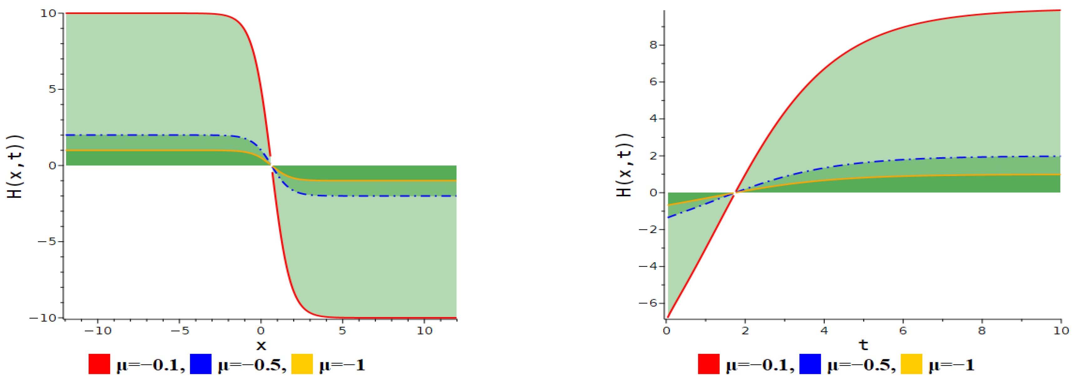
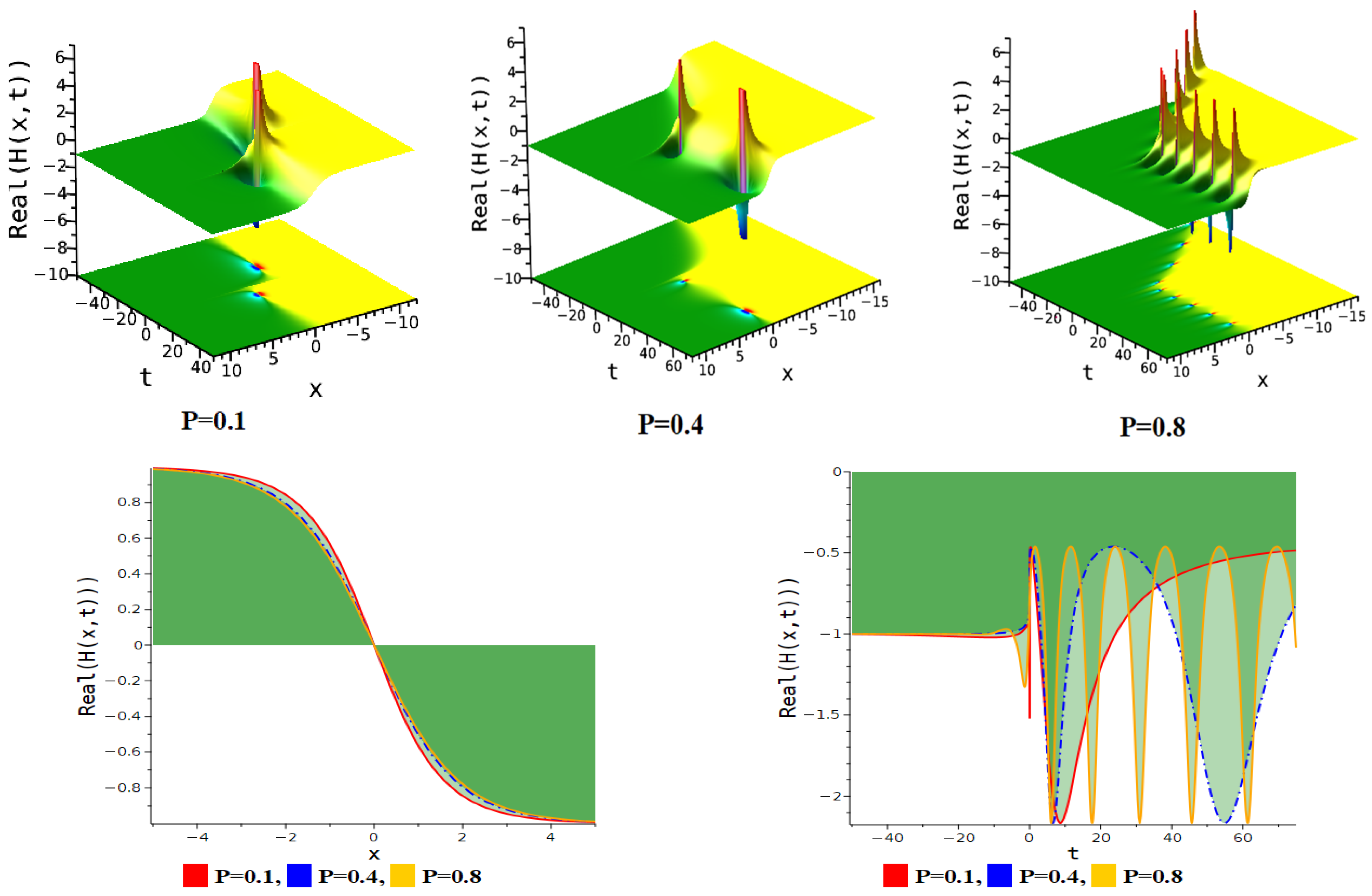
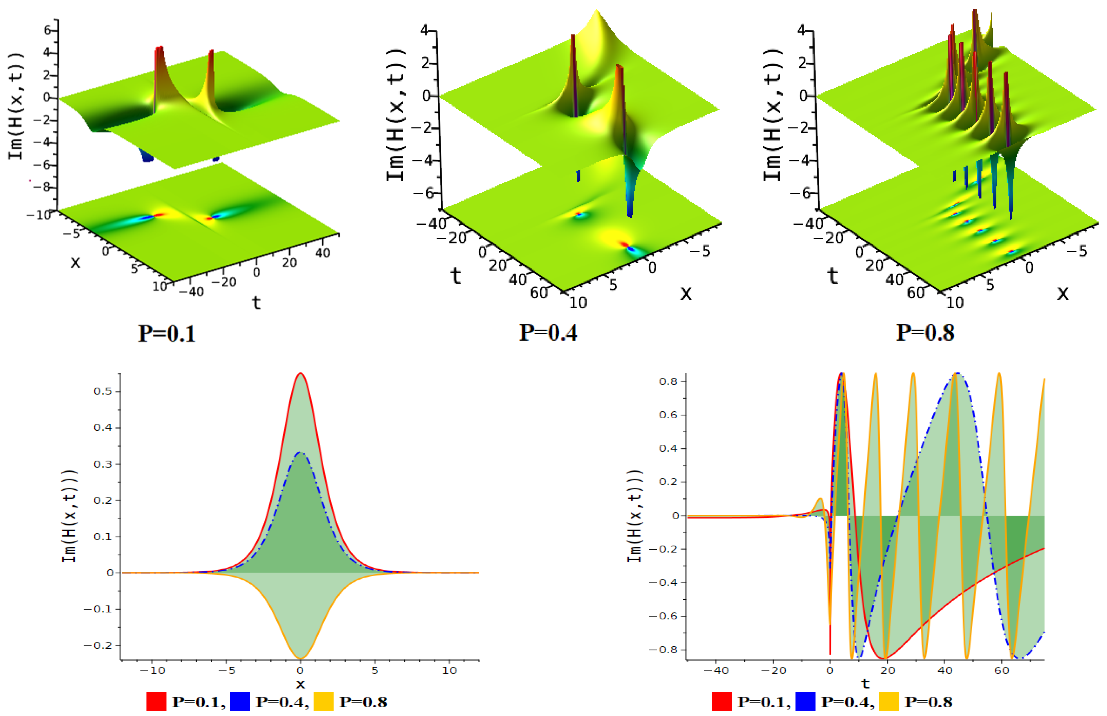
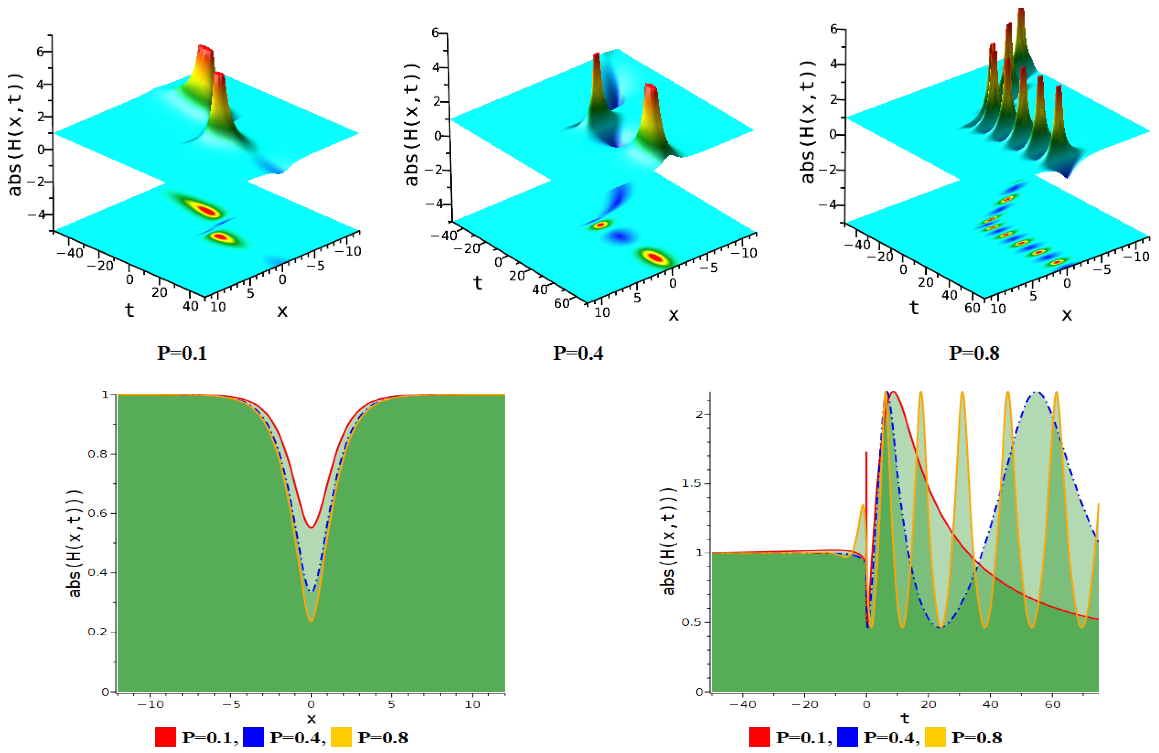
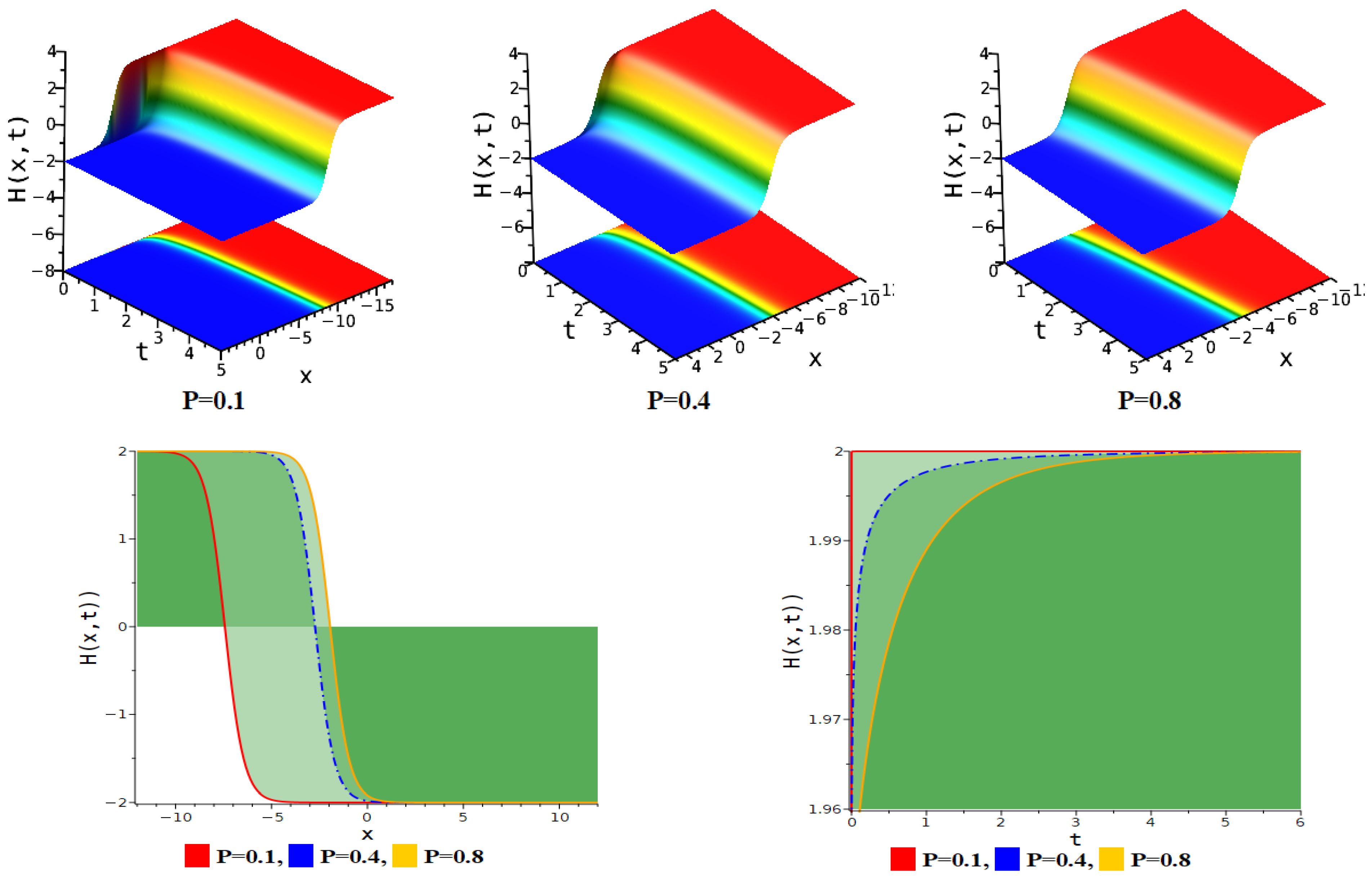
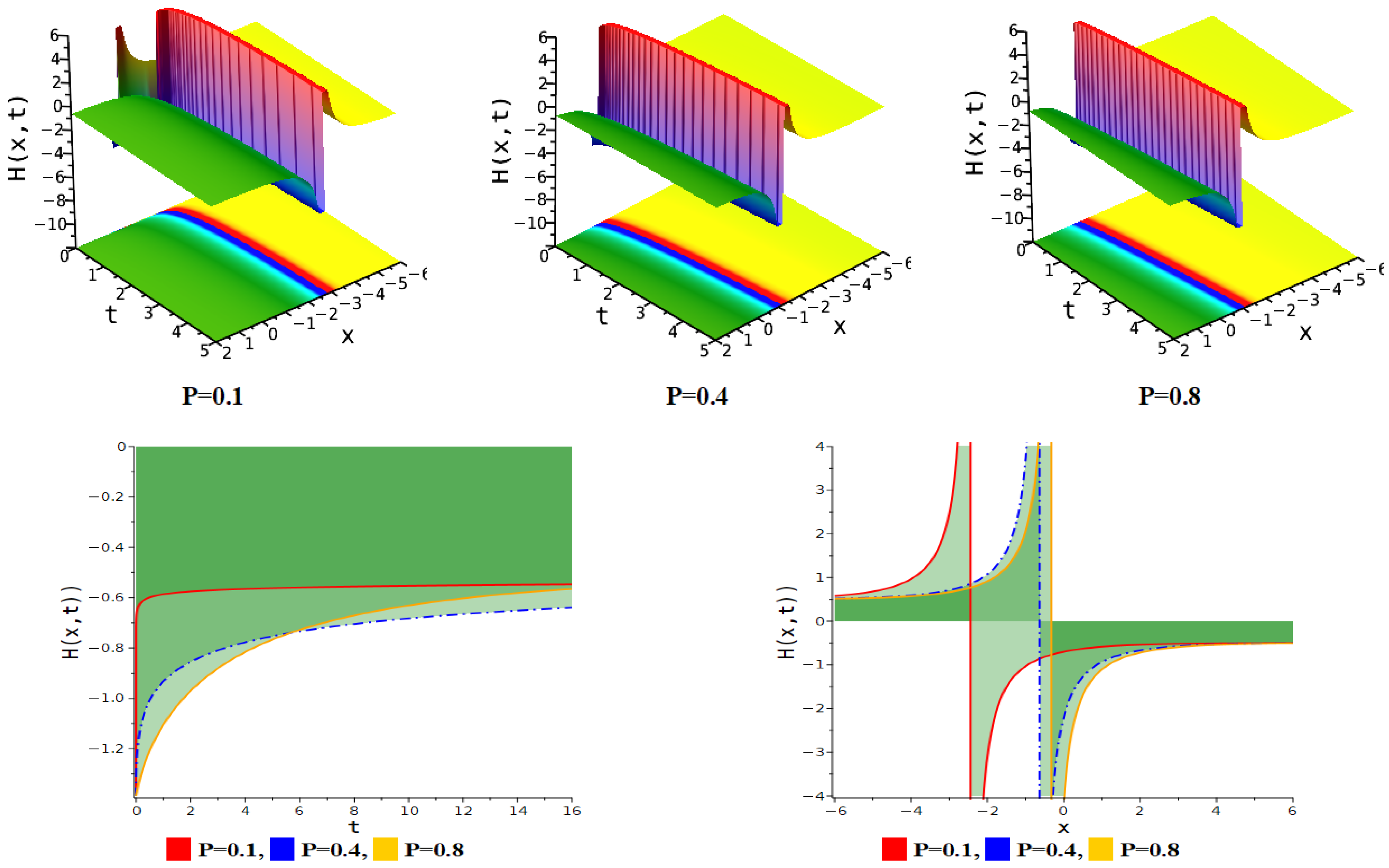
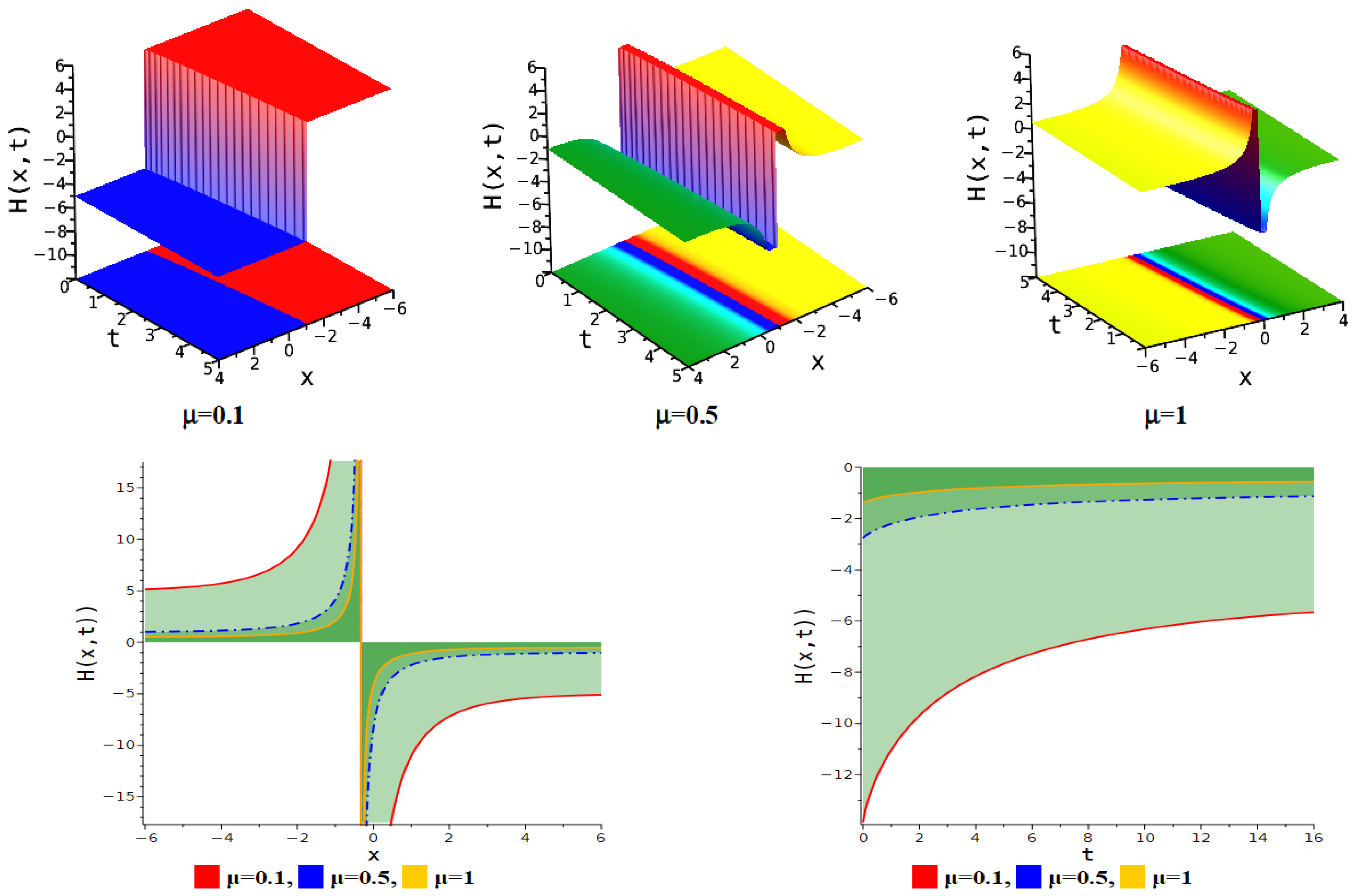
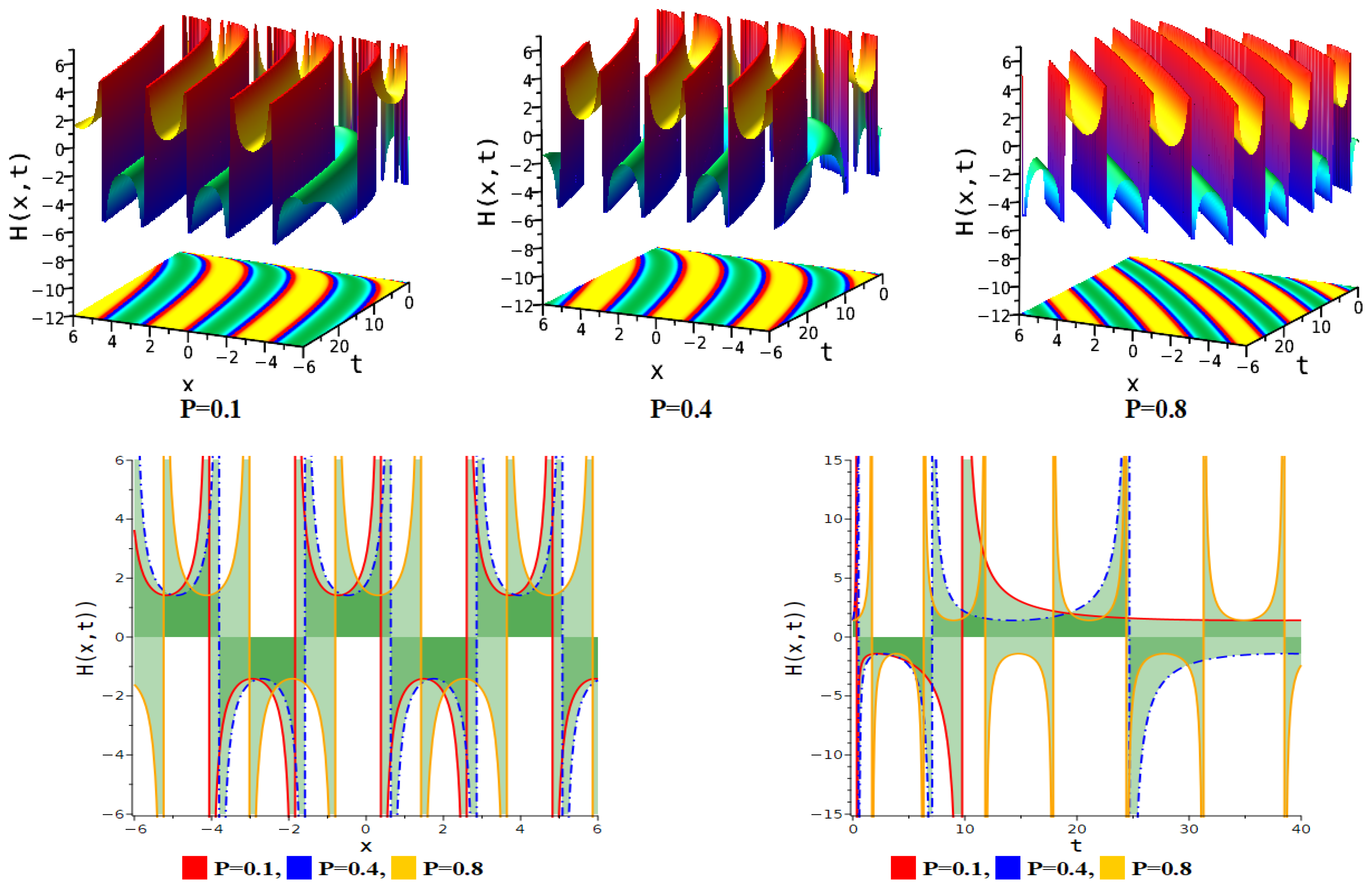
| Figure Type | Corresponding Equation | Parameter Values |
|---|---|---|
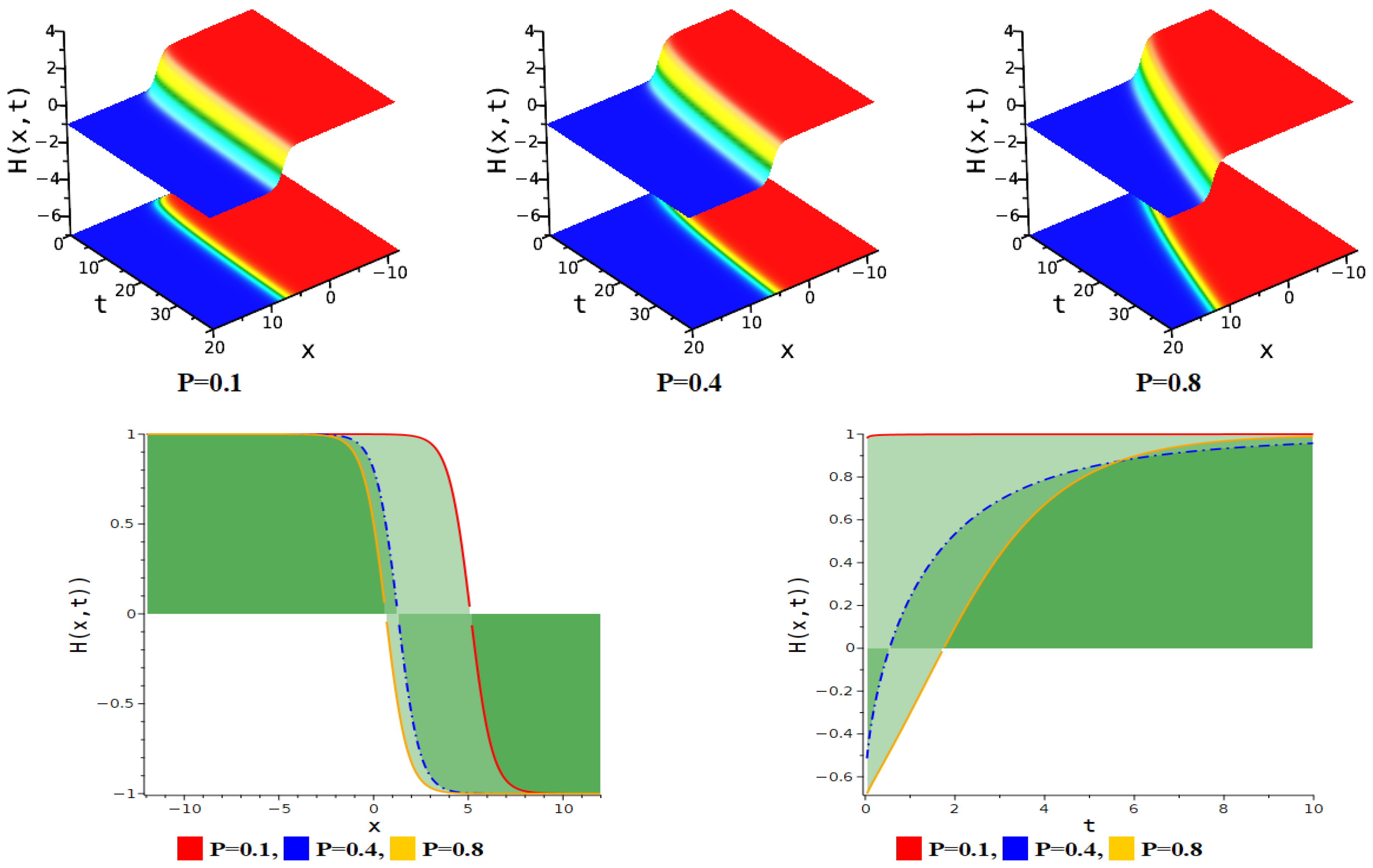
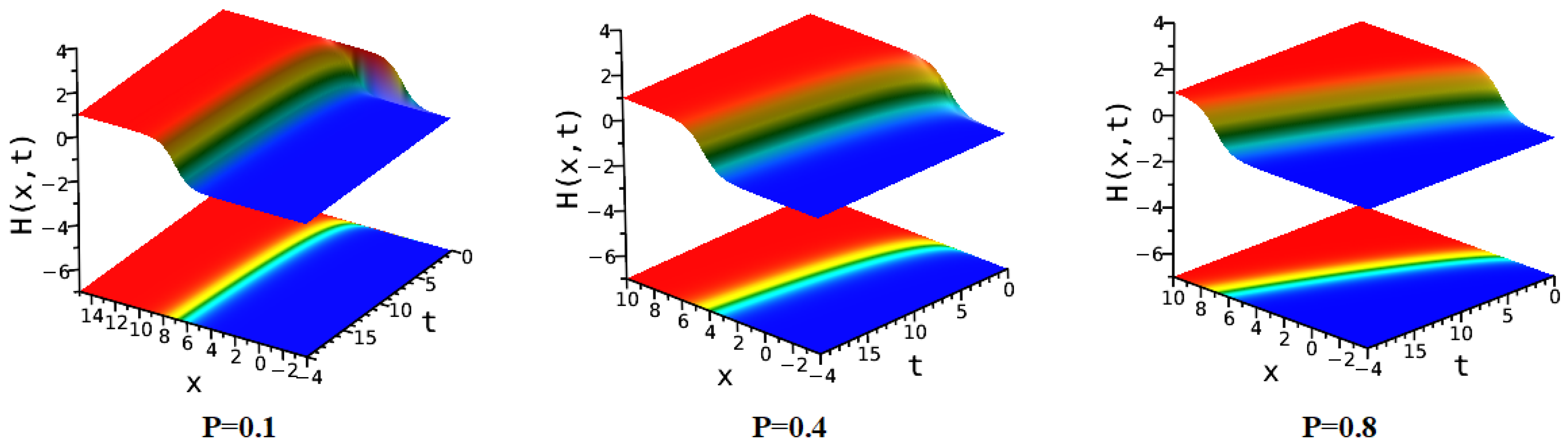
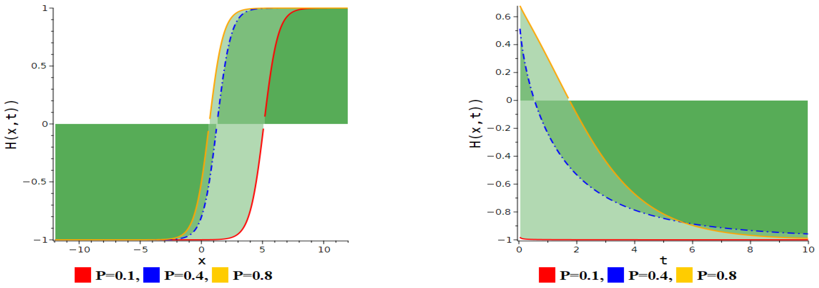
| Anti-kink soliton | Equation (11) | . |
| Kink soliton | Equation (11) | . |
| Interaction between anti-kink and periodic lump soliton | Equation (14) | . |
| Periodic linked-lump soliton | Equation (14) | . |
| Interaction between anti-kink and periodic lump soliton | Equation (14) | . |
| Interaction between anti-kink and periodic lump soliton. | Equation (14) | . |
| Singular soliton | Equation (24) | . |
| Bright periodic soliton | Equation (30) | . |
| Periodic multi-lump soliton | Equation (30) | . |
Disclaimer/Publisher’s Note: The statements, opinions and data contained in all publications are solely those of the individual author(s) and contributor(s) and not of MDPI and/or the editor(s). MDPI and/or the editor(s) disclaim responsibility for any injury to people or property resulting from any ideas, methods, instructions or products referred to in the content. |
© 2025 by the authors. Licensee MDPI, Basel, Switzerland. This article is an open access article distributed under the terms and conditions of the Creative Commons Attribution (CC BY) license (https://creativecommons.org/licenses/by/4.0/).
Share and Cite
Abdalla, M.; Roshid, M.M.; Uddin, M.; Ullah, M.S. Analysis Modulation Instability and Parametric Effect on Soliton Solutions for M-Fractional Landau–Ginzburg–Higgs (LGH) Equation Through Two Analytic Methods. Fractal Fract. 2025, 9, 154. https://doi.org/10.3390/fractalfract9030154
Abdalla M, Roshid MM, Uddin M, Ullah MS. Analysis Modulation Instability and Parametric Effect on Soliton Solutions for M-Fractional Landau–Ginzburg–Higgs (LGH) Equation Through Two Analytic Methods. Fractal and Fractional. 2025; 9(3):154. https://doi.org/10.3390/fractalfract9030154
Chicago/Turabian StyleAbdalla, Mohamed, Md. Mamunur Roshid, Mahtab Uddin, and Mohammad Safi Ullah. 2025. "Analysis Modulation Instability and Parametric Effect on Soliton Solutions for M-Fractional Landau–Ginzburg–Higgs (LGH) Equation Through Two Analytic Methods" Fractal and Fractional 9, no. 3: 154. https://doi.org/10.3390/fractalfract9030154
APA StyleAbdalla, M., Roshid, M. M., Uddin, M., & Ullah, M. S. (2025). Analysis Modulation Instability and Parametric Effect on Soliton Solutions for M-Fractional Landau–Ginzburg–Higgs (LGH) Equation Through Two Analytic Methods. Fractal and Fractional, 9(3), 154. https://doi.org/10.3390/fractalfract9030154