Finite-Time Stability of Fractional-Order Switched Systems Based on Lyapunov Method

Abstract

This paper investigates the finite-time stability of a class of fractional-order switched systems with order $0<\alpha <1$, employing the fractional Lyapunov direct method. First, based on the Mittag-Leffler function and Gronwall inequality, two corresponding sufficient conditions are presented to ensure the finite-time stability of the considered system. Second, in consideration of the effectiveness of dwell time technique in switched systems, a sufficient condition is derived under a minimum average dwell time constraint. Finally, numerical simulations are performed to validate the effectiveness of the theoretical formulation.

1. Introduction

Recently, fractional calculus has emerged as a highly favored extension of classical calculus, owing to its unique advantages in the fields of mathematics and engineering. On the one hand, fractional calculus has gradually penetrated into various disciplines, including anomalous diffusion, non-Newtonian fluid mechanics, viscoelastic materials, and quantum information [1,2]. On the other hand, it is also widely used in machinery and its automation, signal processing and control, biological engineering, and several application fields [3,4,5]. In particular, fractional calculus has become an important mathematical tool for modeling differential equations of complex mechanical phenomena and related stability problems; controller synthesis for fractional-order systems have been intensively investigated, as evidenced by the works of [6,7,8,9,10,11].

As another critical model for investigating complex systems, switched systems have also attracted increasing attention [12,13]. In general, a switched system contains multiple subsystems and a switching rule that designates which subsystem will be adopted at each instant of time along the system trajectory. By means of a common Lyapunov function and less conservative multiple Lyapunov functions combined with dwell time and (mode-based) average dwell time techniques, stability issues of switched systems have obtained a series of fruitful research results [14,15,16].

Specifically, once a switched system incorporates at least one fractional-order subsystem, it is referred to as a fractional-order switched system. Importantly, considering the aberration phenomenon associated with fractional operators [17], it is essential to recognize that the state of a fractional-order switched system is featured by its global nature, with properties that are both history-dependent and non-local. Consequently, the straightforward application of the multiple Lyapunov functions methods, which are conventionally used for aforementioned integer-order switched systems, encounters considerable challenges when adapted to the fractional-order case.

In our previous study [18], a common misinterpretation that arises in fractional-order switched systems’ stability analysis issues was observed. It is crucial to emphasize that once one follows the running order to independently investigate each subsystem, which means the derivative on interval $(t_k,t_{k+1}]$ for a fractional subsystem is taken as ${}_{t_k}{}^{C}D_t^{\alpha }$, the whole system’s memory from $t_0$ to $t_k$ will be neglected. As a matter of fact, the time lower bound of a fractional operator should not be updated with the occurrence of switched behaviors, and the correct notation for each sub-interval should consistently be ${}_{t_0}{}^{C}D_t^{\alpha }$, as applicable to both subsystem modeling and Lyapunov function construction.

As is well known, the fractional Lyapunov direct method presented in [6] establishes a universal approach to address the stability of a fractional system, rather than relying on its differential equation’s explicit solution. Motivated by the aforementioned analysis, this study aims to extend Lyapunov’s theory to address the finite-time stability of fractional-order switched systems involving the correct Caputo fractional derivative notation ${}_{t_0}{}^{C}D_t^{\alpha }$. Significantly, finite-time stability differs from the traditional concept of asymptotic stability, the former primarily concentrates on the system’s dynamics within a finite-time interval. In essence, a system is considered to be finite-time stable if, given that the initial conditions are within a defined boundary, its state remains below a certain threshold throughout a specified time interval [19].

This paper is arranged as follows: Section 2 introduces the preliminaries and problem statement, with remarks provided to illustrate the memory property of fractional operators. The main results are developed in Section 3; by means of the fractional Lyapunov direct method, three sufficient conditions are presented to guarantee the finite-time stability of a class of fractional-order switched systems. In Section 4, numerical examples are given to validate the feasibility of the proposed conditions. Finally, Section 5 summarizes this paper.

Notations.${\mathbb{R}}^n$ denotes n-dimensional real vectors’ space, and for $\forall x\in {\mathbb{R}}^n$, $\Vert x\Vert$ refers to its Euclidean norm $\Vert x\Vert ={\left({\sum }_{i=1}^n{x}_i^2\right)}^{{\displaystyle \frac{1}{2}}}$. ${\mathbb{R}}^{n\times s}$ indicates the space of $n\times s$ real matrices. $L_p[a,b]:=\{f:[a,b]\to \mathbb{R}$; f is measurable on $[a,b]$ and ${\int }_a^b{\left|f\left(x\right)\right|}^{p}dx<\infty$}. $A^n[a,b]$ indicates a space of functions which possess absolutely continuous $(n-1)\mathrm{st}$ derivatives; whenever $f\in A^n[a,b]$, it implies $g=f^{\left(n\right)}$, where $g\in L_1[a,b]$. $\mathcal{L}\left[f\right(t\left)\right]$ represents the Laplace transform of function $f:[0,\infty )\to \mathbb{R}$.

2. Preliminaries and Problem Statement

2.1. Fractional Calculus

Conceptually, fractional calculus is a branch of mathematics used to extend ordinary calculus, which involves the integration and derivation of arbitrary orders, theorized in the 19th century by Riemann and Liouville. However, it is not suitable to utilize Laplace’s transform technique to deal with Riemann–Liouville fractional differential operators, although it is more suitable from a purely mathematical viewpoint. To overcome its fractional initial condition drawbacks, another classical fractional operator was correspondingly given by Caputo in 1969, which clarifies the initial conditions through analogy with the traditional integer-order differential equation.

Definition 1 

([20]). Let $\alpha >0$; the fractional integral of $f\left(t\right)\in L_1[0,\infty )$ is defined by

$${}_{0}D_t^{-\alpha }f\left(t\right)={\displaystyle \frac{1}{\mathrm{\Gamma }\left(\alpha \right)}}{\int }_0^t{\displaystyle \frac{f\left(\tau \right)}{{(t-\tau )}^{1-\alpha }}}\mathrm{d}\tau ,$$

(1)

where $\mathrm{\Gamma }\left(s\right)={\int }_0^{\infty }{e}^{-t}{t}^{s-1}\mathrm{d}t,s\in \mathbb{C},\hspace{1em}Re\left(s\right)>0$ is gamma function.

Definition 2 

([20]). Let $\alpha >0$; the Caputo fractional derivative of $f\left(t\right)\in A^n[0,\infty )$ is defined by

$${}_0{}^{C}D_t^{\alpha }f\left(t\right)={\displaystyle \frac{1}{\mathrm{\Gamma }(n-\alpha )}}{\int }_0^t{\displaystyle \frac{f^{\left(n\right)}\left(\tau \right)}{{(t-\tau )}^{1+\alpha -n}}}\mathrm{d}\tau ,$$

(2)

where n is a positive integer satisfying $n-1<\alpha \le n,n\in {\mathbb{Z}}^{+}$.

Specifically, when $0<\alpha <1$, the Caputo fractional derivative of $f\left(t\right)\in A^1[0,\infty )$ is given by

$${}_0{}^{C}D_t^{\alpha }f\left(t\right)={\displaystyle \frac{1}{\mathrm{\Gamma }(1-\alpha )}}{\int }_0^t{\displaystyle \frac{f^{\prime }\left(\tau \right)}{{(t-\tau )}^{\alpha }}}\mathrm{d}\tau ,$$

(3)

Remark 1. 

In virtue of convolution operation, it is easy to show that the fractional integral in (1) can be represented as ${}_{0}D_t^{-\alpha }f\left(t\right)={\displaystyle \frac{t^{\alpha -1}}{\mathrm{\Gamma }\left(\alpha \right)}}\ast f\left(t\right)$ and that the Caputo fractional derivative in (3) can be expressed as ${}_0{}^{C}D_t^{\alpha }f\left(t\right)={\displaystyle \frac{t^{-\alpha }}{\mathrm{\Gamma }(1-\alpha )}}\ast f^{\prime }\left(t\right)$. Moreover, based on the known Laplace transform property $\mathcal{L}[f_1\left(t\right)\ast f_2\left(t\right)]=\mathcal{L}\left[f_1\left(t\right)\right]\mathcal{L}\left[f_2\left(t\right)\right]$, we can derive that for an arbitrary order, $\alpha >0$, $\mathcal{L}\left[{}_{0}D_t^{-\alpha }f\left(t\right)\right]=s^{-\alpha }F\left(s\right)$, which coincides with the classical integer-order integral. Meanwhile, in the case of $0<\alpha <1$, this implies $\mathcal{L}\left[{}_0{}^{C}D_t^{\alpha }f\left(t\right)\right]=s^{\alpha }F\left(s\right)-s^{\alpha -1}f\left(0\right)$, which is also consistent with the results in traditional integer-order calculus $\mathcal{L}\left[f^{\prime }\left(t\right)\right]=sF\left(s\right)-f\left(0\right)$. Thus, in view of frequency domain theory and physical interpretations for initial conditions, the Caputo fractional operator is always adopted in system control and engineering fields.

Remark 2. 

It can be observed from the above definitions that fractional operators in essence possess non-locality and historical dependence. Specially, to illustrate this issue, in [18], an interesting characteristic of fractional integrals for piecewise functions has been revealed. According to the Heaviside step function, the additivity of integration on intervals is not applicable to fractional integrals.

Lemma 1 

([18]). Suppose that

$$f\left(t\right)=\left\{\begin{array}{c}{f}_1\left(t\right),\hspace{1em}0\le t<t_1,\hfill \\ f_2\left(t\right),\hspace{1em}t\ge t_1,\hfill \end{array}\right.$$

(4)

where $f_1\ne 0$. In general,

$${}_{0}D_t^{-\alpha }f\left(t\right)\ne {}_{0}D_{t_1}^{-\alpha }{f}_1\left(t\right)+{}_{t_1}D_t^{-\alpha }{f}_2\left(t\right),\hspace{1em}\alpha >0,$$

(5)

even if $f_1=f_2.$ It holds that

$${}_{0}D_t^{-\alpha }f\left(t\right)={}_{0}D_t^{-\alpha }{f}_1\left(t\right)+{}_{t_1}D_t^{-\alpha }[f_2\left(t\right)-f_1\left(t\right)],\hspace{1em}\alpha >0.$$

(6)

Proof. 

By utilizing the Heaviside step function,

$$H\left(t\right)=\left\{\begin{array}{c}0,\hspace{1em}t<0,\hfill \\ 1,\hspace{1em}t\ge 0,\hfill \end{array}\right.$$

(7)

$f\left(t\right)$ in (4) yields

$$f\left(t\right)=f_1\left(t\right)\times [H\left(t\right)-H(t-t_1)]+f_2\left(t\right)\times H(t-t_1).$$

(8)

For the first interval, $H\left(t\right)=1,H(t-t_1)=0$ ensures that $f\left(t\right)=f_1\left(t\right),0\le t<t_1$. And for the second interval, $H\left(t\right)=H(t-t_1)=1$ ensures that $f\left(t\right)=f_2\left(t\right),t\ge t_1$.

Taking ${}_{0}D_t^{-\alpha }$ to both sides of (8), it holds that

$$\begin{array}{cc}\hfill {}_{0}D_t^{-\alpha }f\left(t\right)=& {}_{0}D_t^{-\alpha }\left\{f_1\left(t\right)\times [H\left(t\right)-H(t-t_1)]\right\}{+}_0{D}_t^{-\alpha }\left[f_2\left(t\right)\times H(t-t_1)\right]\hfill \\ \hfill =& {}_{0}D_t^{-\alpha }{f}_1\left(t\right)-{{}_{t_1}D_t}^{-\alpha }{f}_1\left(t\right)+{{}_{t_1}D_t}^{-\alpha }{f}_2\left(t\right)\hfill \\ \hfill =& {}_{0}D_t^{-\alpha }{f}_1\left(t\right)+{{}_{t_1}D_t}^{-\alpha }[f_2\left(t\right)-f_1\left(t\right)].\hfill \end{array}$$

□

Lemma 2 

([20]). Consider a Caputo fractional differential equation described as

$$\begin{array}{c}\hfill {}_0{}^{C}D_t^{\alpha }x\left(t\right)=f(t,x\left(t\right)),x\left(0\right)=x_0,\end{array}$$

(9)

where $0<\alpha <1$, and then $x\left(t\right)$ is a solution of problem (9) if and only if $x\left(t\right)$ is a solution of the following nonlinear Volterra integral equation:

$$\begin{array}{c}\hfill x\left(t\right)=x_0+{\displaystyle \frac{1}{\mathrm{\Gamma }\left(\alpha \right)}}{\int }_0^t{(t-\tau )}^{\alpha -1}f(\tau ,x\left(\tau \right))\mathrm{d}\tau .\end{array}$$

(10)

Remark 3. 

In fact, Equation (10) also holds when $\alpha =1$. Now, consider two different instants $t_1$ and $t_2$ with $t_1<t_2$; it can be obtained from (10) that

$$x\left(t_2\right)-x\left(t_1\right)={\displaystyle \frac{1}{\mathrm{\Gamma }\left(\alpha \right)}}{\int }_0^{t_2}{(t_2-\tau )}^{\alpha -1}f(\tau ,x\left(\tau \right))\mathrm{d}\tau -{\displaystyle \frac{1}{\mathrm{\Gamma }\left(\alpha \right)}}{\int }_0^{t_1}{(t_1-\tau )}^{\alpha -1}f(\tau ,x\left(\tau \right))\mathrm{d}\tau ,$$

(11)

using the additivity of integration on intervals for the first integral, we can obtain

$$\begin{array}{cc}\hfill x\left(t_2\right)=& x\left(t_1\right)+{\displaystyle \frac{1}{\mathrm{\Gamma }\left(\alpha \right)}}{\int }_0^{t_1}\left[{(t_2-\tau )}^{\alpha -1}-{(t_1-\tau )}^{\alpha -1}\right]f(\tau ,x\left(\tau \right))\mathrm{d}\tau \hfill \\ \hfill \hspace{1em}& +{\displaystyle \frac{1}{\mathrm{\Gamma }\left(\alpha \right)}}{\int }_{t_1}^{t_2}{(t_2-\tau )}^{\alpha -1}f(\tau ,x\left(\tau \right))\mathrm{d}\tau .\hfill \end{array}$$

(12)

When $\alpha =1$, it holds from the above equation that

$$x\left(t_2\right)=x\left(t_1\right)+{\displaystyle \frac{1}{\mathrm{\Gamma }\left(\alpha \right)}}{\int }_{t_1}^{t_2}f(\tau ,x\left(\tau \right))\mathrm{d}\tau ,$$

which demonstrates that if $x\left(t_1\right)$ is known, one can take $x\left(t_1\right)$ as an initial value for interval $[t_1,t_2]$ to obtain its solution for $t_2>t_1$. Thus, it is unnecessary to use any information on $x\left(t\right)$ for $t\in [0,t_1)$, which essentially verifies the locality of the integer-order differential operators.

However, when $0<\alpha <1$, the issue is fundamentally different since the first integral in (12) always exists. Hence, if one addresses the solution $x\left(t_2\right)$, all information of x from 0 up to the current instant $t_2$ must be considered. This key characteristic reflects the non-locality and long-process memory of the fractional operator ${}_0{}^{C}D_t^{\alpha }$ and verifies that $x\left(t\right)$ is a global variable that contains all historical information.

From the other viewpoint, if (11) is represented as

$$\begin{array}{cc}\hfill x\left(t_2\right)=& \hspace{1em}x\left(t_1\right)-{\displaystyle \frac{1}{\mathrm{\Gamma }\left(\alpha \right)}}{\int }_0^{t_1}{(t_1-\tau )}^{\alpha -1}f(\tau ,x\left(\tau \right))\mathrm{d}\tau +{\displaystyle \frac{1}{\mathrm{\Gamma }\left(\alpha \right)}}{\int }_0^{t_2}{(t_2-\tau )}^{\alpha -1}f(\tau ,x\left(\tau \right))\mathrm{d}\tau \hfill \\ \hfill =& \hspace{1em}{x}_0+{\displaystyle \frac{1}{\mathrm{\Gamma }\left(\alpha \right)}}{\int }_0^{t_2}{(t_2-\tau )}^{\alpha -1}f(\tau ,x\left(\tau \right))\mathrm{d}\tau ,\hfill \end{array}$$

which means that one will always be forced back to the initial value $x_0$ from the known solution $x\left(t_1\right)$, and then take the fractional integral ${}_{0}D_{t_2}^{-\alpha }$ to derive the current solution $x\left(t_2\right)$.

2.2. Finite-Time Stability of Fractional-Order Switched Systems

For a class of fractional-order switched continuous-time system,

$${}_0{}^{C}D_t^{\alpha }x\left(t\right)=A_{\sigma \left(t\right)}x\left(t\right),$$

(13)

where $0<\alpha <1$, $x\left(t\right)\in {\mathbb{R}}^n$ is the system state and $A_{\sigma \left(t\right)}\in {\mathbb{R}}^{n\times n}$ are constant matrices. $\sigma \left(t\right):[0,T]⟶S=\{1,2,···,N\}$ is a time-dependent switching law which is piecewise constant and right continuous, where N denotes the total number of subsystems.

In the following, to avoid Zeno behavior, which means that there is switching behavior with an infinite number in a finite-time interval [21], it is assumed that the considered system (13) occurs n times in the interval $[0,T].$ Then, the switching sequence is denoted as

$$\left\{(\sigma \left(t_1\right),t_1),(\sigma \left(t_2\right),t_2),\cdots ,(\sigma \left(t_k\right),t_k),\cdots ,(\sigma \left(t_n\right),t_n)\right\}$$

where $\sigma \left(t_k\right)=i_k\in S,k=1,\cdots ,n,0<t_1<t_2<\cdots <t_n<T$ and $t_k$ represents the k-th switching instant. For $t\in [t_k,t_{k+1})$, this yields that $i_k$-th subsystem is activated.

As illustrated in [18], even when $t\in [t_k,t_{k+1})$, the Caputo notation should be ${}_0{}^{C}D_t^q$, not ${}_{t_k}{}^{C}D_t^q$, which implies that for $t\in [t_k,t_{k+1})$, the subsystem’s model should be ${}_0{}^{C}D_t^{\alpha }x\left(t\right)=A_{k+1}x\left(t\right),$ where for the simplicity of notation and analysis, the k-th subsystem’s matrix is denoted by $A_k$. That is to say, in a finite-time interval $[0,T]$, the considered system (13) possesses the following form:

$${}_0{}^{C}D_t^{\alpha }x\left(t\right)=\left\{\begin{array}{c}{A}_{1}x\left(t\right),\hspace{1em}0\le t<t_1,\hfill \\ A_{2}x\left(t\right),\hspace{1em}{t}_1\le t<t_2,\hfill \\ A_{3}x\left(t\right),\hspace{1em}{t}_2\le t<t_3,\hfill \\ \hspace{1em}⋮\hfill \\ A_{n+1}x\left(t\right),\hspace{1em}{t}_n\le t\le T.\hfill \end{array}\right.$$

(14)

Meanwhile, suppose that no switching behavior arises at $t=0$ and $t=T$. Then, according to the Heaviside function, an equivalent integral for the system (14) is derived in [18].

Lemma 3 

([18]). Let $0<\alpha <1$, a function $x\in P{C}^1([0,T],{\mathbb{R}}^n)\left(\rho \right)$ is a solution to (14) if and only if $x\in P{C}^1([0,T],{\mathbb{R}}^n)\left(\rho \right)$ is a solution to a fractional integral issue defined by

$$x\left(t\right)=\left\{\begin{array}{c}x\left(0\right)+{\displaystyle \frac{1}{\mathrm{\Gamma }\left(\alpha \right)}}{\int }_0^t{(t-\tau )}^{\alpha -1}{A}_{1}x\left(\tau \right)\mathrm{d}\tau ,\hspace{1em}\hspace{1em}\hspace{1em}\hspace{1em}\hspace{1em}\hspace{1em}\hspace{1em}\hspace{1em}\hspace{1em}\hspace{1em}\hspace{1em}t\in \left[0,t_1\right),\hfill \\ x\left(0\right)+{\displaystyle \frac{1}{\mathrm{\Gamma }\left(\alpha \right)}}{\int }_0^t{(t-\tau )}^{\alpha -1}{A}_{1}x\left(\tau \right)\mathrm{d}\tau +{\displaystyle \frac{1}{\mathrm{\Gamma }\left(\alpha \right)}}{\int }_{t_1}^t{(t-\tau )}^{\alpha -1}(A_2-A_1)x\left(\tau \right)\mathrm{d}\tau ,\hfill \\ \hspace{1em}\hspace{1em}\hspace{1em}\hspace{1em}\hspace{1em}\hspace{1em}\hspace{1em}\hspace{1em}\hspace{1em}\hspace{1em}\hspace{1em}\hspace{1em}\hspace{1em}\hspace{1em}\hspace{1em}\hspace{1em}\hspace{1em}\hspace{1em}\hspace{1em}\hspace{1em}\hspace{1em}\hspace{1em}\hspace{1em}\hspace{1em}\hspace{1em}t\in \left[t_1,t_2\right),\hfill \\ x\left(0\right)+{\displaystyle \frac{1}{\mathrm{\Gamma }\left(\alpha \right)}}{\int }_0^t{(t-\tau )}^{\alpha -1}{A}_{1}x\left(\tau \right)\mathrm{d}\tau +{\displaystyle \frac{1}{\mathrm{\Gamma }\left(\alpha \right)}}{\int }_{t_1}^t{(t-\tau )}^{\alpha -1}(A_2-A_1)x\left(\tau \right)\mathrm{d}\tau \hfill \\ \hspace{1em}\hspace{1em}+{\displaystyle \frac{1}{\mathrm{\Gamma }\left(\alpha \right)}}{\int }_{t_2}^t{(t-\tau )}^{\alpha -1}(A_3-A_2)x\left(\tau \right)\mathrm{d}\tau ,\hspace{1em}\hspace{1em}\hspace{1em}\hspace{1em}\hspace{1em}\hspace{1em}\hspace{0.5em}\hspace{1em}t\in \left[t_2,t_3\right),\hfill \\ \hspace{0.5em}\hspace{1em}⋮\hfill \\ x\left(0\right)+{\displaystyle \frac{1}{\mathrm{\Gamma }\left(\alpha \right)}}{\int }_0^t{(t-\tau )}^{\alpha -1}{A}_{1}x\left(\tau \right)\mathrm{d}\tau \hfill \\ \hspace{1em}\hspace{1em}+{\displaystyle \sum _{k=1}^n}{\displaystyle \frac{1}{\mathrm{\Gamma }\left(\alpha \right)}}{\int }_{t_k}^t{(t-\tau )}^{\alpha -1}(A_{k+1}-A_k)x\left(\tau \right)\mathrm{d}\tau ,\hspace{0.5em}\hspace{1em}\hspace{1em}\hspace{1em}\hspace{1em}t\in \left[t_n,T\right].\hfill \end{array}\right.$$

(15)

Remark 4. 

Inspired by the illustrative statement in Remark 3, we consider a similar issue. For example, choose a specific moment $t^{\prime }\in [t_1,t_2)$; then, we can obtain its corresponding state as the following form:

$$\begin{array}{cc}\hfill x\left(t^{\prime }\right)=& x\left(0\right)+{\displaystyle \frac{1}{\mathrm{\Gamma }\left(\alpha \right)}}{\int }_0^{t^{\prime }}{(t^{\prime }-\tau )}^{\alpha -1}{A}_{1}x\left(\tau \right)\mathrm{d}\tau \hfill \\ \hfill \hspace{1em}& +{\displaystyle \frac{1}{\mathrm{\Gamma }\left(\alpha \right)}}{\int }_{t_1}^{t^{\prime }}{(t^{\prime }-\tau )}^{\alpha -1}(A_2-A_1)x\left(\tau \right)\mathrm{d}\tau ,\hfill \end{array}$$

(16)

we should notice that if $A_1=A_2$, which means it backs to a linear fractional-order system without switching, then the above equation is consistent with (13). But more generally, if we rewrite (16) as

$$x\left(t^{\prime }\right)=x\left(0\right)+{\displaystyle \frac{1}{\mathrm{\Gamma }\left(\alpha \right)}}{\int }_0^{t_1}{(t^{\prime }-\tau )}^{\alpha -1}{A}_{1}x\left(\tau \right)\mathrm{d}\tau +{\displaystyle \frac{1}{\mathrm{\Gamma }\left(\alpha \right)}}{\int }_{t_1}^{t^{\prime }}{(t^{\prime }-\tau )}^{\alpha -1}{A}_{2}x\left(\tau \right)\mathrm{d}\tau ,$$

(17)

compared with the known expression in the traditional integer-order switched system

$$x\left(t^{\prime }\right)=x\left(0\right)+{\displaystyle \frac{1}{\mathrm{\Gamma }\left(\alpha \right)}}{\int }_0^{t_1}{(t_1-\tau )}^{\alpha -1}{A}_{1}x\left(\tau \right)\mathrm{d}\tau +{\displaystyle \frac{1}{\mathrm{\Gamma }\left(\alpha \right)}}{\int }_{t_1}^{t^{\prime }}{(t^{\prime }-\tau )}^{\alpha -1}{A}_{2}x\left(\tau \right)\mathrm{d}\tau ,$$

(18)

this indicates that the non-locality of the fractional operator is embodied in the first integral of (17), since in this item, the function under the integral operation relies on $t^{\prime }$.

As is well known, it is significant to consider a system’s stability. So far, there exists a great number of results on fractional systems’ asymptotic stability. However, in some practical cases, it is unreasonable and not permitted to use too large values of system states [22]. Therefore, it is necessary to concern the transient performance of a system over a finite interval, which is defined as finite-time stability.

Definition 3 

([19]). For the considered system (14), if it holds that

$$\Vert x\left(0\right)\Vert \le c_1⟹\Vert x\left(t\right)\Vert <c_2$$

for $t\in [0,T]$, where $c_2>c_1>0$, then the system (14) is finite-time stable with respect to $(c_1,c_2,T)$.

In [18], according to the presented Volterra integral form in (15), two finite-time stability conditions for fractional-order switched systems are established from its system state perspective. Due to fact that stability analysis based on Lyapunov functions is also an important method with more general applicability, in this paper, we will focus on exploring the corresponding criteria by virtue of the fractional Lyapunov direct method, which will be presented in the next section. Next, some necessary lemmas are introduced below for proofs of these main theorems.

Lemma 4 

([23]). For nonnegative and locally integrable on $[0,T)$ functions $x\left(t\right)$ and $f\left(t\right)$, a nonnegative, nondecreasing continuous function $g\left(t\right)$ with $g\left(t\right)\le M\left(\mathrm{constant}\right),t\in [0,T)$. If it holds for $\alpha >0$ that

$$x\left(t\right)\le f\left(t\right)+g\left(t\right){\int }_0^t{(t-s)}^{\alpha -1}x\left(s\right)\mathrm{d}s,$$

then

$$x\left(t\right)\le f\left(t\right)+{\int }_0^t\left[\sum _{n=1}^{\infty }{\displaystyle \frac{{\left[g\left(t\right)\mathrm{\Gamma }\left(\alpha \right)\right]}^n}{\mathrm{\Gamma }\left(n\alpha \right)}}{(t-s)}^{n\alpha -1}f\left(s\right)\right]\mathrm{d}s.$$

Furthermore, if $f\left(t\right)$ is nondecreasing, then it holds that

$$x\left(t\right)\le f\left(t\right)E_{\alpha }\left[g\left(t\right)\mathrm{\Gamma }\left(\alpha \right)t^{\alpha }\right],$$

where $E_{\alpha }(·)$ denotes the Mittag-Leffler function, defined as $E_{\alpha }\left(z\right)={\displaystyle \sum _{k=0}^{\infty }}{\displaystyle \frac{z^k}{\mathrm{\Gamma }(k\alpha +1)}}$, $\alpha >0$.

Lemma 5 

([24]). For real-valued piecewise-continuous functions, $a\left(t\right)$, $b\left(t\right)$, and $g\left(t\right),t\in [0,T)$. If $b\left(t\right)$ is non-negative and $g\left(t\right)$ satisfies

$$g\left(t\right)\le a\left(t\right)+{\int }_{t_0}^{t}b\left(s\right)g\left(s\right)ds,$$

then

$$g\left(t\right)\le a\left(t\right)+{\int }_{t_0}^{t}a\left(s\right)b\left(s\right)exp\left\{{\int }_s^{t}b\left(r\right)dr\right\}ds.$$

Moreover, if $a\left(t\right)$ is nondecreasing, then it yields

$$g\left(t\right)\le a\left(t\right)exp\left\{{\int }_{t_0}^{t}b\left(s\right)ds\right\}.$$

Lemma 6 

([6]). Let $x\left(0\right)=y\left(0\right)$ and ${}_0{}^{C}D_t^{\alpha }x\left(t\right)\ge {}_0{}^{C}D_t^{\alpha }y\left(t\right)$, where $0<\alpha <1$. Then, $x\left(t\right)\ge y\left(t\right)$.

3. Main Results

For the fractional-order switched system (14), consider the following multiple Lyapunov functions:

$${}_0{}^{C}D_t^{\alpha }V\left(t\right)=\left\{\begin{array}{c}{\lambda }_{1}V\left(t\right),\hspace{1em}0\le t<t_1,\hfill \\ {\lambda }_{2}V\left(t\right),\hspace{1em}{t}_1\le t<t_2,\hfill \\ {\lambda }_{3}V\left(t\right),\hspace{1em}{t}_2\le t<t_3,\hfill \\ \hspace{0.5em}⋮\hfill \\ {\lambda }_{n+1}V\left(t\right),\hspace{0.5em}{t}_n\le t\le T.\hfill \end{array}\right.$$

(19)

Similarly to the derived form in (15), straightforward calculations imply that $V\left(t\right)$ satisfies the following integral equation:

$$V\left(t\right)=\left\{\begin{array}{c}V\left(0\right)+{\displaystyle \frac{{\lambda }_1}{\mathrm{\Gamma }\left(\alpha \right)}}{\int }_0^t{(t-\tau )}^{\alpha -1}V\left(\tau \right)\mathrm{d}\tau ,\hspace{1em}\hspace{1em}\hspace{1em}\hspace{1em}\hspace{1em}\hspace{1em}\hspace{1em}\hspace{1em}\hspace{1em}\hspace{0.5em}\hspace{1em}t\in \left[0,t_1\right),\hfill \\ V\left(0\right)+{\displaystyle \frac{{\lambda }_1}{\mathrm{\Gamma }\left(\alpha \right)}}{\int }_0^t{(t-\tau )}^{\alpha -1}V\left(\tau \right)\mathrm{d}\tau +{\displaystyle \frac{{\lambda }_2-{\lambda }_1}{\mathrm{\Gamma }\left(\alpha \right)}}{\int }_{t_1}^t{(t-\tau )}^{\alpha -1}V\left(\tau \right)\mathrm{d}\tau ,\hfill \\ \hspace{1em}\hspace{1em}\hspace{1em}\hspace{1em}\hspace{1em}\hspace{1em}\hspace{1em}\hspace{1em}\hspace{1em}\hspace{1em}\hspace{1em}\hspace{1em}\hspace{1em}\hspace{1em}\hspace{1em}\hspace{1em}\hspace{1em}\hspace{1em}\hspace{1em}\hspace{1em}\hspace{1em}\hspace{1em}\hspace{1em}\hspace{1em}t\in \left[t_1,t_2\right),\hfill \\ V\left(0\right)+{\displaystyle \frac{{\lambda }_1}{\mathrm{\Gamma }\left(\alpha \right)}}{\int }_0^t{(t-\tau )}^{\alpha -1}V\left(\tau \right)\mathrm{d}\tau +{\displaystyle \frac{{\lambda }_2-{\lambda }_1}{\mathrm{\Gamma }\left(\alpha \right)}}{\int }_{t_1}^t{(t-\tau )}^{\alpha -1}V\left(\tau \right)\mathrm{d}\tau \hfill \\ \hspace{1em}\hspace{1em}+{\displaystyle \frac{{\lambda }_3-{\lambda }_2}{\mathrm{\Gamma }\left(\alpha \right)}}{\int }_{t_2}^t{(t-\tau )}^{\alpha -1}V\left(\tau \right)\mathrm{d}\tau ,\hspace{0.5em}\hspace{1em}\hspace{1em}\hspace{1em}\hspace{1em}\hspace{1em}\hspace{1em}\hspace{1em}\hspace{1em}\hspace{1em}t\in \left[t_2,t_3\right),\hfill \\ \hspace{1em}\hspace{0.5em}⋮\hfill & \hfill \\ V\left(0\right)+{\displaystyle \frac{{\lambda }_1}{\mathrm{\Gamma }\left(\alpha \right)}}{\int }_0^t{(t-\tau )}^{\alpha -1}x\left(\tau \right)\mathrm{d}\tau +{\displaystyle \sum _{k=1}^n}{\displaystyle \frac{{\lambda }_{k+1}-{\lambda }_k}{\mathrm{\Gamma }\left(\alpha \right)}}{\int }_{t_k}^t{(t-\tau )}^{\alpha -1}V\left(\tau \right)\mathrm{d}\tau ,\hfill \\ \hspace{0.5em}\hspace{0.5em}\hspace{1em}\hspace{1em}\hspace{1em}\hspace{1em}\hspace{1em}\hspace{1em}\hspace{1em}\hspace{1em}\hspace{1em}\hspace{1em}\hspace{1em}\hspace{1em}\hspace{1em}\hspace{1em}\hspace{1em}\hspace{1em}\hspace{1em}\hspace{1em}\hspace{1em}\hspace{1em}\hspace{1em}\hspace{1em}\hspace{1em}t\in \left[t_n,T\right].\hfill \end{array}\right.$$

(20)

Next, according to the fractional Lyapunov direct method, three theorems are devoted to verifying the finite-time stability of the considered system (14).

Theorem 1. 

Assume that there exists a continuously differential function $V\left(t\right)$ satisfying locally Lipschitz conditions, scalars ${\lambda }_i>0$, and class-$\mathcal{K}$ functions ${\gamma }_1$ and ${\gamma }_2$, satisfying

$${\gamma }_1(\Vert x\left(t\right)\Vert )\le V\left(t\right)\le {\gamma }_2(\Vert x\left(t\right)\Vert ),$$

(21)

$${}_0{}^{C}D_t^{\alpha }V\left(t\right)\le {\lambda }_i{\gamma }_1(\Vert x\left(t\right)\Vert ),$$

(22)

$${\gamma }_2\left(c_1\right)E_{\alpha }\left({\lambda }_{max}{T}^{\alpha }\right)<{\gamma }_1\left(c_2\right),$$

(23)

where ${\lambda }_{max}=\underset{i\in S}{max}\left\{{\lambda }_i\right\}$, then the system (14) is finite-time stable with respect to $(c_1,c_2,T)$.

Proof. 

According to conditions (21) and (22), one obtains

$${}_0{}^{C}D_t^{\alpha }V\left(t\right)\le {\lambda }_{i}V\left(t\right).$$

(24)

Based on the fractional comparison principle in Lemma 6, considering the following comparison system:

$${}_0{}^{C}D_t^{\alpha }V\left(t\right)={\lambda }_{i}V\left(t\right),$$

(25)

and recalling the derived equivalent integral in (20), when $t\in [0,t_1)$, one has

$$V\left(t\right)=V\left(0\right)+{\displaystyle \frac{1}{\mathrm{\Gamma }\left(\alpha \right)}}{\int }_0^t{(t-\tau )}^{\alpha -1}{\lambda }_{1}V\left(\tau \right)\mathrm{d}\tau ,$$

(26)

then, by virtue of Lemma 4, one can directly obtain the following inequality:

$$V\left(t\right)\le V\left(0\right)E_{\alpha }\left({\displaystyle \frac{{\lambda }_1}{\mathrm{\Gamma }\left(\alpha \right)}}\mathrm{\Gamma }\left(\alpha \right)t^{\alpha }\right)\le V\left(0\right)E_{\alpha }\left({\lambda }_{max}{T}^{\alpha }\right).$$

(27)

If $t\in [t_1,t_2)$, taking into account the Heaviside function $H\left(t\right)$, one has

$$\begin{array}{c}\hfill {}_0{}^{C}D_t^{\alpha }V\left(t\right)={\lambda }_{1}V\left(t\right)[H\left(t\right)-H(t-t_1)]+{\lambda }_{2}V\left(t\right)H(t-t_1),\end{array}$$

(28)

integrating both sides of (28) from 0 to t, it yields

$$\begin{array}{cc}\hfill V\left(t\right)=& V\left(0\right)+{\displaystyle \frac{1}{\mathrm{\Gamma }\left(\alpha \right)}}{\int }_0^t{(t-\tau )}^{\alpha -1}\{{\lambda }_{1}V\left(\tau \right)[H\left(\tau \right)-H(\tau -t_1)]\hfill \\ \hfill \hspace{1em}& +{\lambda }_{2}V\left(\tau \right)H(\tau -t_1)\}\mathrm{d}\tau \hfill \\ \hfill \le & V\left(0\right)+{\displaystyle \frac{{\lambda }_{max}}{\mathrm{\Gamma }\left(\alpha \right)}}{\int }_0^t{(t-\tau )}^{\alpha -1}V\left(\tau \right)\mathrm{d}\tau ,\hfill \end{array}$$

(29)

then it can be derived from Lemma 4 that

$$\begin{array}{c}\hfill V\left(t\right)\le V\left(0\right)E_{\alpha }\left({\lambda }_{max}{T}^{\alpha }\right).\end{array}$$

(30)

Proceeding as in the above technique, if $t\in [t_{k-1},t_k)$, based on

$$\begin{array}{cc}\hfill {}_0{}^{C}D_t^{\alpha }V\left(t\right)=& {\lambda }_{1}V\left(t\right)[H\left(t\right)-H(t-t_1)]+{\lambda }_{2}V\left(t\right)[H(t-t_1)-H(t-t_2)]+\cdots \hfill \\ \hfill & +{\lambda }_{k-1}V\left(t\right)[H(t-t_{k-2})-H(t-t_{k-1})]+{\lambda }_{k}V\left(t\right)H(t-t_{k-1}),\hfill \end{array}$$

(31)

one can obtain

$$\begin{array}{cc}\hfill V\left(t\right)\le & V\left(0\right)+{\displaystyle \frac{{\lambda }_{max}}{\mathrm{\Gamma }\left(\alpha \right)}}{\int }_0^t{(t-\tau )}^{\alpha -1}V\left(\tau \right)\mathrm{d}\tau ,\hfill \end{array}$$

(32)

then it holds from Lemma 4 that

$$\begin{array}{c}\hfill V\left(t\right)\le V\left(0\right)E_{\alpha }\left({\lambda }_{max}{T}^{\alpha }\right).\end{array}$$

(33)

Consequently, if $\Vert x\left(0\right)\Vert \le c_1$, then it follows from the given conditions (21)–(23) that

$$\begin{array}{cc}\hfill \Vert x\left(t\right)\Vert \le & {\gamma }_1^{-1}\left(V\left(t\right)\right)\le {\gamma }_1^{-1}\left(V\left(0\right)E_{\alpha }\left({\lambda }_{max}{T}^{\alpha }\right)\right)\hfill \\ \hfill \le & {\gamma }_1^{-1}({\gamma }_2(\Vert x\left(0\right)\Vert )E_{\alpha }\left({\lambda }_{max}{T}^{\alpha }\right))\hfill \\ \hfill \le & {\gamma }_1^{-1}\left({\gamma }_2\left(c_1\right)E_{\alpha }\left({\lambda }_{max}{T}^{\alpha }\right)\right)\hfill \\ \hfill <& c_2.\hfill \end{array}$$

(34)

By Definition 3, the finite-time stability of the considered system (14) can be guaranteed with respect to $(c_1,c_2,T)$. □

Remark 5. 

In fact, if we consider a fractional-order system without switching behavior, then the presented condition from (21) to (23) can be returned to the existing result in Theorem 1 in [25], which addresses the finite-time stability criteria for fractional nonlinear systems ${}_0{}^{C}D_t^{\alpha }x\left(t\right)=f(t,x\left(t\right))$.

Theorem 2. 

Assume that there exists a continuously differential function $V\left(t\right)$ satisfying the locally Lipschitz condition, scalars ${\lambda }_i>0$, and class-$\mathcal{K}$ functions ${\gamma }_1$ and ${\gamma }_2$, satisfying

$${\gamma }_1(\Vert x\left(t\right)\Vert )\le V\left(t\right)\le {\gamma }_2(\Vert x\left(t\right)\Vert ),$$

(35)

$${}_0{}^{C}D_t^{\alpha }V\left(t\right)\le {\lambda }_i{\gamma }_1(\Vert x\left(t\right)\Vert ),$$

(36)

$$T<{\left({\displaystyle \frac{\mathrm{\Gamma }(\alpha +1)}{{\lambda }_{max}}}\left[ln{\gamma }_1\left(c_2\right)-ln{\gamma }_2\left(c_1\right)\right]\right)}^{{\displaystyle \frac{1}{\alpha }}},$$

(37)

where ${\lambda }_{max}=\underset{i\in S}{max}\left\{{\lambda }_i\right\}$; then, the system (14) is finite-time stable with respect to $(c_1,c_2,T)$.

Proof. 

Proceeding in a similar technique to the aforementioned, let us begin once again with the following comparison system:

$${}_0{}^{C}D_t^{\alpha }V\left(t\right)={\lambda }_{i}V\left(t\right).$$

(38)

If $t\in [0,t_1)$, taking ${}_{0}D_t^{-\alpha }$ to both sides, one obtains

$$V\left(t\right)=V\left(0\right)+{\displaystyle \frac{1}{\mathrm{\Gamma }\left(\alpha \right)}}{\int }_0^t{(t-\tau )}^{\alpha -1}{\lambda }_{1}V\left(\tau \right)\mathrm{d}\tau ,$$

(39)

based on Lemma 5, this implies

$$\begin{array}{cc}\hfill V\left(t\right)\le V\left(0\right)exp\left\{{\displaystyle \frac{{\lambda }_1}{\mathrm{\Gamma }\left(\alpha \right)}}{\int }_0^t{(t-\tau )}^{\alpha -1}\mathrm{d}\tau \right\}=& V\left(0\right)exp\left\{{\displaystyle \frac{{\lambda }_1{t}^{\alpha }}{\mathrm{\Gamma }(\alpha +1)}}\right\}\hfill \\ \hfill \le & V\left(0\right)exp\left\{{\displaystyle \frac{{\lambda }_{max}{T}^{\alpha }}{\mathrm{\Gamma }(\alpha +1)}}\right\}.\hfill \end{array}$$

(40)

If $t\in [t_1,t_2)$, according to the Heaviside function $H\left(t\right)$, its equation can be expressed as

$$\begin{array}{c}\hfill {}_0{}^{C}D_t^{\alpha }V\left(t\right)={\lambda }_{2}V\left(t\right)={\lambda }_{1}V\left(t\right)[H\left(t\right)-H(t-t_1)]+{\lambda }_{2}V\left(t\right)H(t-t_1),\end{array}$$

(41)

applying the same order fractional integral ${}_{0}D_t^{-\alpha }$ to both sides of (41), by means of Lemma 5, implies

$$\begin{array}{cc}\hfill V\left(t\right)=& V\left(0\right)+{\displaystyle \frac{1}{\mathrm{\Gamma }\left(\alpha \right)}}{\int }_0^t{(t-\tau )}^{\alpha -1}\{{\lambda }_{1}V\left(\tau \right)[H\left(\tau \right)-H(\tau -t_1)]\hfill \\ \hfill \hspace{1em}& +{\lambda }_{2}V\left(\tau \right)H(\tau -t_1)\}\mathrm{d}\tau ,\hfill \\ \hfill \le & V\left(0\right)exp\left\{{\displaystyle \frac{1}{\mathrm{\Gamma }\left(\alpha \right)}}{\int }_0^t{(t-\tau )}^{\alpha -1}\{{\lambda }_1[H\left(\tau \right)-H(\tau -t_1)]+{\lambda }_{2}H(\tau -t_1)\}\mathrm{d}\tau \right\}\hfill \\ \hfill \le & V\left(0\right)exp\left\{{\displaystyle \frac{{\lambda }_1}{\mathrm{\Gamma }\left(\alpha \right)}}{\int }_0^t{(t-\tau )}^{\alpha -1}\mathrm{d}\tau +{\displaystyle \frac{{\lambda }_2-{\lambda }_1}{\mathrm{\Gamma }\left(\alpha \right)}}{\int }_{t_1}^t{(t-\tau )}^{\alpha -1}\mathrm{d}\tau \right\}\hfill \\ \hfill =& V\left(0\right)exp\left\{{\displaystyle \frac{1}{\mathrm{\Gamma }(\alpha +1)}}\left[{\lambda }_1{t}^{\alpha }+({\lambda }_2-{\lambda }_1){(t-t_1)}^{\alpha }\right]\right\}\hfill \\ \hfill \le & V\left(0\right)exp\left\{{\displaystyle \frac{{\lambda }_2{T}^{\alpha }}{\mathrm{\Gamma }(\alpha +1)}}\right\}\hfill \\ \hfill \le & V\left(0\right)exp\left\{{\displaystyle \frac{{\lambda }_{max}{T}^{\alpha }}{\mathrm{\Gamma }(\alpha +1)}}\right\}.\hfill \end{array}$$

(42)

Similarly, if $t\in [t_{k-1},t_k)$, it implies

$$\begin{array}{cc}\hfill V\left(t\right)\le & V\left(0\right)exp\{{\displaystyle \frac{1}{\mathrm{\Gamma }(\alpha +1)}}[{\lambda }_1{t}^{\alpha }+({\lambda }_2-{\lambda }_1){(t-t_1)}^{\alpha }+\cdots \hfill \\ \hfill & +({\lambda }_k-{\lambda }_{k-1}){(t-t_{k-1})}^{\alpha }]\}\hfill \\ \hfill \le & V\left(0\right)exp\left\{{\displaystyle \frac{1}{\mathrm{\Gamma }(\alpha +1)}}\left[{\lambda }_1{T}^{\alpha }+({\lambda }_2-{\lambda }_1)T^{\alpha }+\cdots +({\lambda }_k-{\lambda }_{k-1})T^{\alpha }\right]\right\}\hfill \\ \hfill =& V\left(0\right)exp\left\{{\displaystyle \frac{{\lambda }_k{T}^{\alpha }}{\mathrm{\Gamma }(\alpha +1)}}\right\}\hfill \\ \hfill \le & V\left(0\right)exp\left\{{\displaystyle \frac{{\lambda }_{max}{T}^{\alpha }}{\mathrm{\Gamma }(\alpha +1)}}\right\}.\hfill \end{array}$$

(43)

That is to say, for any sub-interval, based on conditions (35) and (36), it holds that

$$\begin{array}{cc}\hfill {\gamma }_1(\Vert x\left(t\right)\Vert )\le V\left(t\right)\le & V\left(0\right)exp\left\{{\displaystyle \frac{{\lambda }_{max}{T}^{\alpha }}{\mathrm{\Gamma }(\alpha +1)}}\right\}\hfill \\ \hfill \le & {\gamma }_2(\Vert x\left(0\right)\Vert )exp\left\{{\displaystyle \frac{{\lambda }_{max}{T}^{\alpha }}{\mathrm{\Gamma }(\alpha +1)}}\right\}\hfill \\ \hfill \le & {\gamma }_2\left(c_1\right)exp\left\{{\displaystyle \frac{{\lambda }_{max}{T}^{\alpha }}{\mathrm{\Gamma }(\alpha +1)}}\right\}.\hfill \end{array}$$

(44)

Therefore, under the restricted condition (37), one can compute that $\Vert x\left(t\right)\Vert <c_2$, $\forall t\ge 0$. Thus, the considered system (14) is also finite-time stable with respect to $(c_1,c_2,T)$. □

In addition, it is worth mentioning that the average dwell time strategy is another important approach to use as a switching scheme. Next, a computable sufficient condition is presented to ensure the finite-time stability of the considered fractional-order switched system with the minimum average dwell time constraint.

Definition 4 

([26]). For any time interval $[t_1,t_2)$ and a switching signal $\sigma \left(t\right)$, let $N_{\sigma }(t_1,t_2)$ denote the switching number of $\sigma \left(t\right)$ over $[t_1,t_2)$. If there exist constants $N_0\ge 0$ and ${\tau }_a>0$ such that

$$N_{\sigma }(t_1,t_2)\le N_0+{\displaystyle \frac{t_2-t_1}{{\tau }_a}},$$

then the positive constant ${\tau }_a$ is called the average dwell time and $N_0$ is called the chatter bound. For the sake of simplicity, we choose $N_0=0$ throughout this paper.

Theorem 3. 

Assume that there exists a continuously differential function $V\left(t\right)$ satisfying the locally Lipschitz condition, scalars ${\lambda }_i>0$, and class-$\mathcal{K}$ functions ${\gamma }_1$ and ${\gamma }_2$, satisfying

$${\gamma }_1(\Vert x\left(t\right)\Vert )\le V\left(t\right)\le {\gamma }_2(\Vert x\left(t\right)\Vert ),$$

(45)

$${}_0{}^{C}D_t^{\alpha }V\left(t\right)\le {\lambda }_i{\gamma }_1(\Vert x\left(t\right)\Vert ),$$

(46)

then under the following constraint for the average dwell time:

$${\displaystyle {\tau }_a>{\tau }_a^{*}=\frac{{\lambda }_{max}{T}^{\alpha +1}}{\mathrm{\Gamma }(\alpha +1)\left[ln{\gamma }_1\left(c_2\right)-ln{\gamma }_2\left(c_1\right)\right]},}$$

(47)

where ${\lambda }_{max}=\underset{i\in S}{max}\left\{{\lambda }_i\right\}$, the considered system (20) is finite-time stable with respect to $(c_1,c_2,T,\sigma )$.

Proof. 

Combining conditions (45), (46), and the fractional comparison principle in Lemma 6 and considering the following comparison system:

$${}_0{}^{C}D_t^{\alpha }V\left(t\right)={\lambda }_{i}V\left(t\right).$$

(48)

If $t\in [0,t_1)$, one has

$$V\left(t\right)=V\left(0\right)+{\displaystyle \frac{1}{\mathrm{\Gamma }\left(\alpha \right)}}{\int }_0^t{(t-\tau )}^{\alpha -1}{\lambda }_{1}V\left(\tau \right)\mathrm{d}\tau ,$$

(49)

then, based on Lemma 5, it is easy to obtain

$$V\left(t\right)\le V\left(0\right)exp\left\{{\displaystyle \frac{{\lambda }_1}{\mathrm{\Gamma }\left(\alpha \right)}}{\int }_0^t{(t-\tau )}^{\alpha -1}\mathrm{d}\tau \right\}=V\left(0\right)exp\left\{{\displaystyle \frac{{\lambda }_1{t}^{\alpha }}{\mathrm{\Gamma }(\alpha +1)}}\right\},$$

(50)

which means that

$$V\left(t_1\right)=V\left(t_1^{-}\right)\le V\left(0\right)exp\left\{{\displaystyle \frac{{\lambda }_1{t}_1^{\alpha }}{\mathrm{\Gamma }(\alpha +1)}}\right\}.$$

(51)

If $t\in [t_1,t_2)$, one has

$$\begin{array}{c}\hfill {}_0{}^{C}D_t^{\alpha }V\left(t\right)={\lambda }_{2}V\left(t\right)={\lambda }_{1}V\left(t\right)[H\left(t\right)-H(t-t_1)]+{\lambda }_{2}V\left(t\right)H(t-t_1),\end{array}$$

(52)

integrating both sides of (52) from 0 to t, based on the given equivalent solution (20), one obtain from the derived $V\left(t\right)$ form in $t\in [t_1,t_2)$ that

$$\begin{array}{cc}\hfill V\left(t\right)=& V\left(0\right)+{\displaystyle \frac{1}{\mathrm{\Gamma }\left(\alpha \right)}}{\int }_0^t{(t-\tau )}^{\alpha -1}\{{\lambda }_{1}V\left(\tau \right)[H\left(\tau \right)-H(\tau -t_1)]\hfill \\ \hfill \hspace{1em}& +{\lambda }_{2}V\left(\tau \right)H(\tau -t_1)\}\mathrm{d}\tau \hfill \\ \hfill =& V\left(t_1\right)-{\displaystyle \frac{{\lambda }_1}{\mathrm{\Gamma }\left(\alpha \right)}}{\int }_0^{t_1}{(t_1-\tau )}^{\alpha -1}V\left(\tau \right)\mathrm{d}\tau -{\displaystyle \frac{{\lambda }_2-{\lambda }_1}{\mathrm{\Gamma }\left(\alpha \right)}}{\int }_{t_1}^{t_1}{(t_1-\tau )}^{\alpha -1}V\left(\tau \right)\mathrm{d}\tau \hfill \\ \hfill & +{\displaystyle \frac{1}{\mathrm{\Gamma }\left(\alpha \right)}}{\int }_0^t{(t-\tau )}^{\alpha -1}\{{\lambda }_{1}V\left(\tau \right)[H\left(\tau \right)-H(\tau -t_1)]+{\lambda }_{2}V\left(\tau \right)H(\tau -t_1)\}\mathrm{d}\tau \hfill \\ \hfill \le & V\left(t_1\right)+{\displaystyle \frac{1}{\mathrm{\Gamma }\left(\alpha \right)}}{\int }_0^t{(t-\tau )}^{\alpha -1}\{{\lambda }_1[H\left(\tau \right)-H(\tau -t_1)]+{\lambda }_{2}H(\tau -t_1)\}V\left(\tau \right)\mathrm{d}\tau .\hfill \end{array}$$

(53)

By Lemma 5, it holds that

$$\begin{array}{cc}\hfill V\left(t\right)\le & V\left(t_1\right)exp\left\{{\displaystyle \frac{1}{\mathrm{\Gamma }\left(\alpha \right)}}{\int }_0^t{(t-\tau )}^{\alpha -1}\{{\lambda }_1[H\left(\tau \right)-H(\tau -t_1)]+{\lambda }_{2}H(\tau -t_1)\}\mathrm{d}\tau \right\}\hfill \\ \hfill \le & V\left(0\right)exp\left\{{\displaystyle \frac{{\lambda }_1{t}_1^{\alpha }}{\mathrm{\Gamma }(\alpha +1)}}\right\}exp\{{\displaystyle \frac{{\lambda }_1}{\mathrm{\Gamma }\left(\alpha \right)}}{\int }_0^t{(t-\tau )}^{\alpha -1}\mathrm{d}\tau \hfill \\ \hfill \hspace{1em}& +{\displaystyle \frac{{\lambda }_2-{\lambda }_1}{\mathrm{\Gamma }\left(\alpha \right)}}{\int }_{t_1}^t{(t-\tau )}^{\alpha -1}\mathrm{d}\tau \}\hfill \\ \hfill =& V\left(0\right)exp\left\{{\displaystyle \frac{1}{\mathrm{\Gamma }(\alpha +1)}}\left[{\lambda }_1(t_1^{\alpha }+t^{\alpha })+({\lambda }_2-{\lambda }_1){(t-t_1)}^{\alpha }\right]\right\},\hfill \end{array}$$

(54)

which means that

$$\begin{array}{cc}\hfill V\left(t_2\right)=V\left(t_2^{-}\right)\le & V\left(0\right)exp\left\{{\displaystyle \frac{1}{\mathrm{\Gamma }(\alpha +1)}}\left[{\lambda }_1(t_1^{\alpha }+t_2^{\alpha })+({\lambda }_2-{\lambda }_1){(t_2-t_1)}^{\alpha }\right]\right\}.\hfill \end{array}$$

(55)

If $t\in [t_2,t_3)$, ${}_0{}^{C}D_t^{\alpha }V\left(t\right)={\lambda }_{3}V\left(t\right)$ can be similarly presented as

$$\begin{array}{cc}\hfill {}_0{}^{C}D_t^{\alpha }V\left(t\right)=& {\lambda }_{1}V\left(t\right)[H\left(t\right)-H(t-t_1)]+{\lambda }_{2}V\left(t\right)[H(t-t_1)-H(t-t_2)]\hfill \\ \hfill \hspace{1em}& +{\lambda }_{3}V\left(t\right)H(t-t_2),\hfill \end{array}$$

(56)

repeating the previous process, under the derived equivalent form (20), $V\left(0\right)$ can be replaced by

$$\begin{array}{cc}\hfill V\left(t\right)=& V\left(0\right)+{\displaystyle \frac{1}{\mathrm{\Gamma }\left(\alpha \right)}}{\int }_0^t{(t-\tau )}^{\alpha -1}\{{\lambda }_{1}V\left(\tau \right)[H\left(\tau \right)-H(\tau -t_1)]+{\lambda }_{2}V\left(\tau \right)[H(\tau -t_1)\hfill \\ \hfill \hspace{1em}& -H(\tau -t_2)]+{\lambda }_{3}V\left(\tau \right)H(\tau -t_2)\}\mathrm{d}\tau \hfill \\ \hfill =& V\left(t_2\right)-{\displaystyle \frac{{\lambda }_1}{\mathrm{\Gamma }\left(\alpha \right)}}{\int }_0^{t_2}{(t_2-\tau )}^{\alpha -1}V\left(\tau \right)\mathrm{d}\tau -{\displaystyle \frac{{\lambda }_2-{\lambda }_1}{\mathrm{\Gamma }\left(\alpha \right)}}{\int }_{t_1}^{t_2}{(t_2-\tau )}^{\alpha -1}V\left(\tau \right)\mathrm{d}\tau \hfill \\ \hfill \hspace{1em}& -{\displaystyle \frac{{\lambda }_3-{\lambda }_2}{\mathrm{\Gamma }\left(\alpha \right)}}{\int }_{t_2}^{t_2}{(t_2-\tau )}^{\alpha -1}V\left(\tau \right)\mathrm{d}\tau +{\displaystyle \frac{1}{\mathrm{\Gamma }\left(\alpha \right)}}{\int }_0^t{(t-\tau )}^{\alpha -1}\{{\lambda }_1[H\left(\tau \right)\hfill \\ \hfill \hspace{1em}& -H(\tau -t_1)]+{\lambda }_2[H(\tau -t_1)-H(\tau -t_2)]+{\lambda }_{3}H(t-t_2)\}V\left(\tau \right)\mathrm{d}\tau \hfill \\ \hfill =& V\left(t_2\right)-{\displaystyle \frac{{\lambda }_1}{\mathrm{\Gamma }\left(\alpha \right)}}{\int }_0^{t_1}{(t_2-\tau )}^{\alpha -1}V\left(\tau \right)\mathrm{d}\tau -{\displaystyle \frac{{\lambda }_2}{\mathrm{\Gamma }\left(\alpha \right)}}{\int }_{t_1}^{t_2}{(t_2-\tau )}^{\alpha -1}V\left(\tau \right)\mathrm{d}\tau \hfill \\ \hfill \hspace{1em}& +{\displaystyle \frac{1}{\mathrm{\Gamma }\left(\alpha \right)}}{\int }_0^t{(t-\tau )}^{\alpha -1}\{{\lambda }_1[H\left(\tau \right)-H(\tau -t_1)]+{\lambda }_2[H(\tau -t_1)-H(\tau -t_2)]\hfill \\ \hfill \hspace{1em}& +{\lambda }_{3}H(\tau -t_2)\}V\left(\tau \right)\mathrm{d}\tau \hfill \\ \hfill \le & V\left(t_2\right)+{\displaystyle \frac{1}{\mathrm{\Gamma }\left(\alpha \right)}}{\int }_0^t{(t-\tau )}^{\alpha -1}\{{\lambda }_1[H\left(\tau \right)-H(\tau -t_1)]+{\lambda }_2[H(\tau -t_1)\hfill \\ \hfill \hspace{1em}& -H(\tau -t_2)]+{\lambda }_{3}H(\tau -t_2)\}V\left(\tau \right)\mathrm{d}\tau ,\hfill \end{array}$$

(57)

based on Lemma 5, one can further obtain that

$$\begin{array}{c}\hfill \begin{array}{cc}\hfill V\left(t\right)\le & V\left(t_2\right)exp\{{\displaystyle \frac{1}{\mathrm{\Gamma }\left(\alpha \right)}}{\int }_0^t{(t-\tau )}^{\alpha -1}\{{\lambda }_1[H\left(\tau \right)-H(\tau -t_1)]+{\lambda }_2[H(\tau -t_1)\hfill \\ & -H(\tau -t_2)]+{\lambda }_{3}H(\tau -t_2)\left\}\mathrm{d}\tau \right\}\hfill \\ \hfill \le & V\left(0\right)exp\left\{{\displaystyle \frac{1}{\mathrm{\Gamma }(\alpha +1)}}\left[{\lambda }_1(t_1^{\alpha }+t_2^{\alpha })+({\lambda }_2-{\lambda }_1){(t_2-t_1)}^{\alpha }\right]\right\}\hfill \\ & ·exp\{{\displaystyle \frac{{\lambda }_1}{\mathrm{\Gamma }\left(\alpha \right)}}{\int }_0^t{(t-\tau )}^{\alpha -1}\mathrm{d}\tau +{\displaystyle \frac{{\lambda }_2-{\lambda }_1}{\mathrm{\Gamma }\left(\alpha \right)}}{\int }_{t_1}^t{(t-\tau )}^{\alpha -1}\mathrm{d}\tau \hfill \\ & +{\displaystyle \frac{{\lambda }_3-{\lambda }_2}{\mathrm{\Gamma }\left(\alpha \right)}}{\int }_{t_2}^t{(t-\tau )}^{\alpha -1}\mathrm{d}\tau \}\hfill \\ \hfill =& V\left(0\right)exp\{{\displaystyle \frac{1}{\mathrm{\Gamma }(\alpha +1)}}\{{\lambda }_1(t_1^{\alpha }+t_2^{\alpha }+t^{\alpha })+({\lambda }_2-{\lambda }_1)[{(t_2-t_1)}^{\alpha }+{(t-t_1)}^{\alpha }]\hfill \\ & +({\lambda }_3-{\lambda }_2){(t-t_2)}^{\alpha }\left\}\right\}.\hfill \end{array}\end{array}$$

(58)

This will then, taking the similar calculations, one can verify that when $t\in [t_{k-1},t_k)$, it follows that

$$\begin{array}{cc}\hfill V\left(t\right)\le & V\left(0\right)exp\{{\displaystyle \frac{1}{\mathrm{\Gamma }(\alpha +1)}}\{{\lambda }_1(t_1^{\alpha }+t_2^{\alpha }+\cdots +t_{k-1}^{\alpha }+t^{\alpha })+({\lambda }_2-{\lambda }_1)[{(t_2-t_1)}^{\alpha }\hfill \\ \hfill \hspace{1em}& +{(t_3-t_1)}^{\alpha }+\cdots +{(t_{k-1}-t_1)}^{\alpha }+{(t-t_1)}^{\alpha }]+\cdots +({\lambda }_{k-1}-{\lambda }_{k-2})\hfill \\ \hfill \hspace{1em}& \left[{(t_{k-1}-t_{k-2})}^{\alpha }+{(t-t_{k-2})}^{\alpha }\right]+({\lambda }_k-{\lambda }_{k-1}){(t-t_{k-1})}^{\alpha }\left\}\right\}\hfill \\ \hfill \le & V\left(0\right)exp\{{\displaystyle \frac{1}{\mathrm{\Gamma }(\alpha +1)}}[k{\lambda }_1{T}^{\alpha }+(k-1)({\lambda }_2-{\lambda }_1)T^{\alpha }+\cdots +2({\lambda }_{k-1}-{\lambda }_{k-2})T^{\alpha }\hfill \\ \hfill \hspace{1em}& +({\lambda }_k-{\lambda }_{k-1})T^{\alpha }\left]\right\}\hfill \\ \hfill =& V\left(0\right)exp\left\{{\displaystyle \frac{({\lambda }_1+{\lambda }_2+\cdots +{\lambda }_k)T^{\alpha }}{\mathrm{\Gamma }(\alpha +1)}}\right\}.\hfill \end{array}$$

(59)

Therefore, it holds for any sub-interval that

$$\begin{array}{cc}\hfill V\left(t\right)\le & V\left(0\right)exp\left\{{\displaystyle \frac{{\lambda }_{max}{N}_{\sigma }{T}^{\alpha }}{\mathrm{\Gamma }(\alpha +1)}}\right\}.\hfill \end{array}$$

(60)

Our next goal is to address the finite-time stability of the studied system. To this end, we note that under the given condition (45), it can be implied that

$$\begin{array}{cc}\hfill {\gamma }_1(\Vert x\left(t\right)\Vert )\le V\left(t\right)\le & V\left(0\right)exp\left\{{\displaystyle \frac{{\lambda }_{max}{N}_{\sigma }{T}^{\alpha }}{\mathrm{\Gamma }(\alpha +1)}}\right\}\hfill \\ \hfill \le & {\gamma }_2(\Vert x\left(0\right)\Vert )exp\left\{{\displaystyle \frac{{\lambda }_{max}{T}^{\alpha +1}}{\mathrm{\Gamma }(\alpha +1){\tau }_a}}\right\}\hfill \\ \hfill \le & {\gamma }_2\left(c_1\right)exp\left\{{\displaystyle \frac{{\lambda }_{max}{T}^{\alpha +1}}{\mathrm{\Gamma }(\alpha +1){\tau }_a}}\right\},\hfill \end{array}$$

(61)

and, based on the average dwell time condition (47), we can derive that

$$\begin{array}{cc}\hfill \Vert x\left(t\right)\Vert \le & {\gamma }_1^{-1}\left({\gamma }_2\left(c_1\right)exp\left\{{\displaystyle \frac{{\lambda }_{max}{T}^{\alpha +1}}{\mathrm{\Gamma }(\alpha +1){\tau }_a}}\right\}\right)\hfill \\ \hfill <& {\gamma }_1^{-1}\left({\gamma }_2\left(c_1\right)exp\left\{ln{\gamma }_1\left(c_2\right)-ln{\gamma }_2\left(c_1\right)\right\}\right)\hfill \\ \hfill =& {\gamma }_1^{-1}\left({\gamma }_1\left(c_2\right)\right)\hfill \\ \hfill =& c_2,\hfill \end{array}$$

(62)

which leads to the required state threshold value condition. □

Remark 6. 

The case when $N_{\sigma }=1$ corresponds to a class of fractional-order systems, which means switching behavior does not exist, then this implies that the derived condition (60) in Theorem 3 can be expressed as

$$\begin{array}{cc}\hfill V\left(t\right)\le & V\left(0\right)exp\left\{{\displaystyle \frac{\lambda T^{\alpha }}{\mathrm{\Gamma }(\alpha +1)}}\right\}.\hfill \end{array}$$

(63)

To derive the boundedness $\Vert x\left(t\right)\Vert <c_2,\forall t\in [0,T]$, taking the similar manipulation from (61) to (62) requires

$${\displaystyle T<{\left(\frac{\mathrm{\Gamma }(\alpha +1)[ln{\gamma }_1\left(c_2\right)-ln{\gamma }_2\left(c_1\right)]}{\lambda }\right)}^{\frac{1}{\alpha }}.}$$

(64)

On the one hand, comparing the above condition with the derived condition in (37) verifies that Theorem 3 is a consistent extension of Theorem 2.

On the other hand, when $N_{\sigma }=1$, combining (64) with (45), (46) is the same as the existing classical results for fractional-order nonlinear systems, which have been presented in Theorem 2 in [25]. As a consequence of this observation, we can derive that Theorems 2 and 3 are generalizations of a single fractional-order system.

4. Numerical Examples

In general, a boost converter is a DC–DC power converter that steps up the voltage from its input to its output, which can be regarded as a class of switched-mode power supply, including at least two semiconductors and at least one energy storage element. If its capacitor or inductor is a fractional-order energy-storage component, then the considered system is a fractional-order switched system.

Meanwhile, it is well known that, in a boost converter, if the current changes too fast, its circuit will break down; thus, it is necessary to study its finite-time stability performance.

Example 1. 

For a fractional-order switched system described by

$${}_0{}^{C}D_t^{\alpha }x\left(t\right)=\left\{\begin{array}{c}0.3x\left(t\right),\hspace{1em}\hspace{1em}0\le t<1,\hfill \\ 0.12x\left(t\right),\hspace{0.5em}\hspace{1em}1\le t\le 3.\hfill \end{array}\right.$$

(65)

Constructing the Lyapunov function as $V\left(t\right)=\left|x\right(t\left)\right|$, it can be calculated that when $0\le t<1$, we have ${}_0{}^{C}D_t^{\alpha }V\left(t\right)=0.3\left|x\left(t\right)\right|$, and when $1\le t\le 3$, this implies that ${}_0{}^{C}D_t^{\alpha }V\left(t\right)=0.12\left|x\left(t\right)\right|.$ By choosing ${\gamma }_1(\Vert x\left(t\right)\Vert )=\left|x\left(t\right)\right|,{\gamma }_2(\Vert x\left(t\right)\Vert )=2\left|x\left(t\right)\right|$, ${\lambda }_1=0.3, {\lambda }_2=0.2$, it can be verified that conditions 1 and 2 in Theorem 2 are satisfied.

The related simulation is carried out by choosing $x\left(0\right)=3$, the relevant parameters are given as $\alpha =0.5, c_1=3, c_2=10, {\lambda }_{max}=0.3$, then it can be calculated from condition 3 in Theorem 2 that

$$T<{\left({\displaystyle \frac{\mathrm{\Gamma }\left(1.5\right)}{0.3}}\left[ln10-ln6\right]\right)}^{{\displaystyle \frac{1}{0.5}}}=2.2772.$$

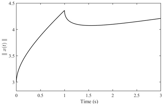
From Figure 1, it can be verified that $\Vert x\left(t\right)\Vert$ does not exceed the given value $c_2$ over 0–2.2772 s, which is to say that the system (65) is finite-time stable with respect to $(c_1,c_2,T)$, where $T<2.2772 s$, which demonstrates the effectiveness of Theorem 2.

Figure 1. The trajectory of $\Vert x\left(t\right)\Vert$ for system (65).

Example 2. 

For a fractional-order switched system described by

$${}_0{}^{C}D_t^{\alpha }x\left(t\right)=A_{\sigma \left(t\right)}x\left(t\right)$$

(66)

where $x\left(t\right)={[x_1\left(t\right),x_2\left(t\right)]}^T\in {\mathbb{R}}^2$ and $\sigma \left(t\right)$ is a switching signal taking value in $S=\{1,2\}$, choose

$$A_1=\left[\begin{array}{cc}1.1& 0.4\\ -2.2& -0.3\end{array}\right],\hspace{1em}{A}_2=\left[\begin{array}{cc}-8& -1.12\\ 1& 1.24\end{array}\right].$$

Constructing the Lyapunov function as $V\left(t\right)= |x_1\left(t\right)|+|x_2\left(t\right)|$, it can be calculated that for the first fractional-order subsystem, we have

$${}_0{}^{C}D_t^{\alpha }V\left(t\right)={}_0{}^{C}D_t^{\alpha }|x_1\left(t\right)|+{}_0{}^{C}D_t^{\alpha }|x_2\left(t\right)|=-1.1|x_1\left(t\right)|+0.1|x_2\left(t\right)|\le 0.1\sqrt{2}\sqrt{x_1^2\left(t\right)+x_2^2\left(t\right)}.$$

Similarly, for the second fractional-order subsystem, it is implied that

$${}_0{}^{C}D_t^{\alpha }V\left(t\right)={}_0{}^{C}D_t^{\alpha }|x_1\left(t\right)|+{}_0{}^{C}D_t^{\alpha }|x_2\left(t\right)|=-7|x_1\left(t\right)|+0.12|x_2\left(t\right)|\le 0.12\sqrt{2}\sqrt{x_1^2\left(t\right)+x_2^2\left(t\right)}.$$

By choosing ${\gamma }_1(\Vert x\left(t\right)\Vert )=\sqrt{x_1^2\left(t\right)+x_2^2\left(t\right)}, {\gamma }_2(\Vert x\left(t\right)\Vert )=2\sqrt{x_1^2\left(t\right)+x_2^2\left(t\right)}$, ${\lambda }_1=0.15, {\lambda }_2=0.18$, the conditions 1 and 2 in Theorem 3 are satisfied.

The relevant parameters for the system (66) are selected as $x\left(0\right)={[0.1,0]}^T$, $\alpha =0.8,$ $c_1=0.1, c_2=100,$ $T=10 s$, ${\lambda }_{max}=0.18$; it can be straightforwardly calculated that

$${\displaystyle {\tau }_a^{*}=\frac{0.18*{10}^{1.8}}{\mathrm{\Gamma }\left(1.8\right)(ln100-ln0.2)}=1.9621.}$$

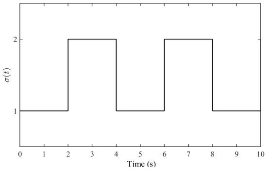
Then, based on condition 3 in Theorem 3, the average dwell time can be given as ${\tau }_a=2 s$. The following Figure 2 shows the switching signal in the numerical simulation.

Figure 2. The switching signal $\sigma \left(t\right)$ with the average dwell time ${\tau }_a=2 s$.

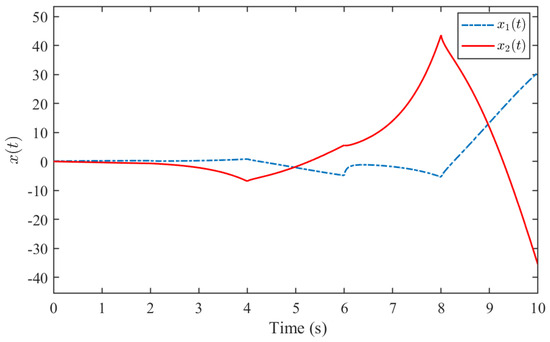
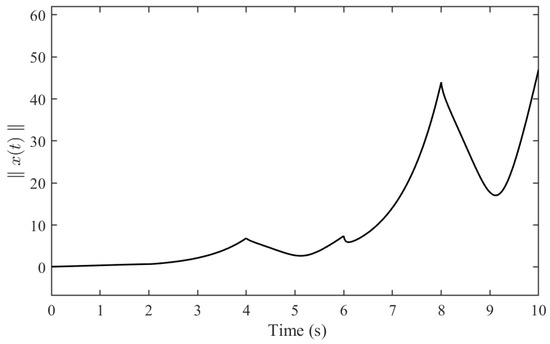
Based on the above given signal, the system state $x\left(t\right)$ and the value of $\Vert x\left(t\right)\Vert$ are depicted in Figure 3 and Figure 4, respectively.

Figure 3. The state response of $x\left(t\right)$ for system (66).

Figure 4. The trajectory of $\Vert x\left(t\right)\Vert$ for system (66).

As shown in Figure 4, $\Vert x\left(t\right)\Vert$ does not exceed the given bound $c_2$ over 0–10 s, which illustrates that the finite-time stability of the considered system can be guaranteed under the designed conditions in Theorem 3.

5. Conclusions

The finite-time stability of a class of fractional-order switched systems with order $0<\alpha <1$ is addressed in this paper. On the one hand, two criteria are established by virtue of the Mittag-Leffler function and Gronwall inequality, respectively. These criteria ensure that the considered system’s state does not exceed a certain threshold over a finite-time interval. On the other hand, recognizing the significance of the average dwell time technique for switched systems, a further sufficient criterion is subsequently derived to ensure the finite-time stability of the considered systems. Future research will focus on the construction of specific Lyapunov candidate functions to derive operative test conditions for stability issues and event-triggered control of fractional-order hybrid systems. Meanwhile, the state-dependent switching control of the considered fractional-order switched system will also be considered.

References

- Metzler, R.; Glöckle, W.G.; Nonnenmacher, T.F. Fractional model equation for anomalous diffusion. Phys. A Stat. Mech. Its Appl. 2012, 211, 13–24. [Google Scholar] [CrossRef]
- Yang, X.; Liang, Y.; Chen, W. A fractal roughness model for the transport of fractional non-Newtonian fluid in microtubes. Chaos Solitons Fractals 2019, 126, 236–241. [Google Scholar] [CrossRef]
- Efe, M.Ö. Fractional order systems in industrial automation—A Survey. IEEE Trans. Ind. Inform. 2011, 7, 582–591. [Google Scholar] [CrossRef]
- Podlubny, I. Fractional-order systems and PIλDμ controllers. IEEE Trans. Autom. Control 1999, 44, 208–214. [Google Scholar] [CrossRef]
- Yu, M.; Li, Y.; Podlubny, I.; Gong, F.; Zhang, C. Fractional-order modeling of lithium-ion batteries using additive noise assisted modeling and correlative information criterion. J. Adv. Res. 2020, 25, 49–56. [Google Scholar] [CrossRef]
- Li, Y.; Chen, Y.Q.; Podlubny, I. Mittag-Leffler stability of fractional order nonlinear dynamic systems. Automatica 2009, 45, 1965–1969. [Google Scholar] [CrossRef]
- Lu, J.; Chen, Y.Q. Robust stability and stabilization of fractional-order interval systems with the fractional order: The case 0 < α < 1. IEEE Trans. Autom. Control 2010, 55, 152–158. [Google Scholar]
- Duarte-Mermoud, M.; Aguila-Camacho, N.; Gallegos, J. Using general quadratic Lyapunov functions to prove Lyapunov uniform stability for fractional order systems. Commun. Nonlinear Sci. Numer. Simul. 2015, 22, 650–659. [Google Scholar] [CrossRef]
- Abolpour, R.; Dehghani, M.; Tavazoei, M.S. Reducing conservatism in robust stability analysis of fractional-order-polytopic systems. ISA Trans. 2021, 119, 106–117. [Google Scholar] [CrossRef]
- Echenausía-Monroy, J.; Huerta-Cuellar, G.; Jaimes-Reátegui, R.; García-López, J.; Aboites, V.; Cassal-Quiroga, B.; Gilardi-Velázquez, H. Multistability emergence through fractional-order-derivatives in a PWL multi-scroll system. Electronics 2020, 9, 880. [Google Scholar] [CrossRef]
- Clemente-López, D.; Munoz-Pacheco, J.; Zambrano-Serrano, E.; Félix Beltrán, O.; Rangel-Magdaleno, J. A piecewise linear approach for implementing fractional-order multi-scroll chaotic systems on ARMs and FPGAs. Fractal Fract. 2024, 8, 389. [Google Scholar] [CrossRef]
- Dai, Y.; Kim, Y.; Wee, S.; Lee, D.; Lee, S. A switching formation strategy for obstacle avoidance of a multi-robot system based on robot priority model. ISA Trans. 2015, 56, 123–134. [Google Scholar] [CrossRef]
- Lee, Y.; Suh, B.; Min, B.W. A Ka-Band bi-directional reconfigurable switched beam-forming network based on 4×4 Butler matrix in 28-nm CMOS. IEEE Trans. Microw. Theory Tech. 2023, 71, 2479–2487. [Google Scholar] [CrossRef]
- Zhao, X.; Yin, Y.; Liu, L.; Sun, X. Stability analysis and delay control for switched positive linear systems. IEEE Trans. Autom. Control 2018, 63, 2184–2190. [Google Scholar] [CrossRef]
- Li, Z.; Zhao, J. Co-design of controllers and a switching policy for non-strict feedback switched nonlinear systems including first-order feedforward paths. IEEE Trans. Autom. Control 2019, 64, 1753–1760. [Google Scholar] [CrossRef]
- Feng, T.; Wu, B.; Wang, Y.E.; Chen, Y.Q. Input-output finite-time stability of switched singular continuous-time systems. Int. J. Control Autom. Syst. 2021, 19, 1828–1835. [Google Scholar] [CrossRef]
- Du, B.; Wei, Y.; Liang, S.; Wang, Y. Estimation of exact initial states of fractional order systems. Nolinear Dyn. 2016, 86, 2061–2070. [Google Scholar] [CrossRef]
- Feng, T.; Guo, L.; Wu, B.; Chen, Y.Q. Stability analysis of switched fractional-order continuous-time systems. Nonlinear Dyn. 2020, 102, 2467–2478. [Google Scholar] [CrossRef]
- Amato, F.; Ariola, M.; Dorato, P. Finite-time control of linear systems subject to parametric uncertainties and disturbances. Automatica 2001, 37, 1459–1463. [Google Scholar] [CrossRef]
- Kilbas, A.A.A.; Srivastava, H.M.; Trujillo, J.J. Theory and Applications of Fractional Differential Equations; Elsevier: New York, NY, USA, 2006. [Google Scholar]
- Zhang, Y.; Wu, H.; Cao, J. Global Mittag-Leffler consensus for fractional singularly perturbed multi-agent systems with discontinuous inherent dynamics via event-triggered control strategy. J. Frankl. Inst. 2021, 358, 2086–2114. [Google Scholar] [CrossRef]
- Ma, Y.; Wu, B.; Wang, Y. Finite-time stability and finite-time boundedness of fractional order linear systems. Neurocomputing 2016, 173, 2076–2082. [Google Scholar] [CrossRef]
- Ye, H.; Gao, J.; Ding, Y. A generalized Gronwall inequality and its application to a fractional differential equation. J. Math. Anal. Appl. 2007, 328, 1075–1081. [Google Scholar] [CrossRef]
- Delavari, H.; Baleanu, D.; Sadati, J. Stability analysis of Caputo fractional-order nonlinear systems. Nonlinear Dyn. 2012, 67, 2433–2439. [Google Scholar] [CrossRef]
- Yang, Y.; Chen, G. Finite-time stability of fractional order impulsive switched systems. Int. J. Robust Nonlinear Control 2015, 25, 2207–2222. [Google Scholar] [CrossRef]
- Zhou, L.; Ho, D.W.C.; Zhai, G. Stability analysis of switched linear singular systems. Automatica 2013, 49, 1481–1487. [Google Scholar] [CrossRef]
Disclaimer/Publisher’s Note: The statements, opinions and data contained in all publications are solely those of the individual author(s) and contributor(s) and not of MDPI and/or the editor(s). MDPI and/or the editor(s) disclaim responsibility for any injury to people or property resulting from any ideas, methods, instructions or products referred to in the content. |
© 2025 by the authors. Licensee MDPI, Basel, Switzerland. This article is an open access article distributed under the terms and conditions of the Creative Commons Attribution (CC BY) license (https://creativecommons.org/licenses/by/4.0/).