Boundary Control for Consensus in Fractional-Order Multi-Agent Systems Under DoS Attacks and Actuator Failures

Abstract

This paper investigates the consensus problem in fractional-order multi-agent systems (FOMASs) under Denial of Service (DoS) attacks and actuator faults. A boundary control strategy is proposed, which reduces dependence on internal sensors and actuators by utilizing only the state information at the system boundaries, significantly lowering control costs. To address DoS attacks, a buffer mechanism is designed to store valid control signals during communication interruptions and apply them once communication is restored, thereby enhancing the system’s robustness and stability. Additionally, this study considers the impact of actuator performance fluctuations on control effectiveness and proposes corresponding adjustment strategies to ensure that the system maintains consensus and stability even in the presence of actuator failures or performance variations. Finally, the effectiveness of the proposed method is validated through numerical experiments. The results show that, even under DoS attacks and actuator faults, the system can still successfully achieve consensus and maintain good stability, demonstrating the feasibility and effectiveness of this control approach in complex environments.

1. Introduction

MASs are systems composed of multiple agents, where each agent is an autonomous entity capable of making its own decisions and interacting with other agents and the environment. With the development of artificial intelligence, communication technologies, sensor technologies, and other fields, MASs have found widespread application in various domains. In robotics and automation, MASs are extensively used in drone swarm collaboration [1], robot formation control [2], and autonomous vehicles [3], where multiple robots collaborate to complete complex tasks. In intelligent transportation systems, MASs are applied in vehicle-to-everything communication [4], intelligent traffic signal control [5], and traffic flow management [6], improving traffic efficiency and safety. In MASs, traditional distributed control methods often face challenges such as communication delays [7], information loss, and reliance on a large number of sensors and actuators, especially as the system size increases or external attacks occur. These issues can lead to reduced control efficiency and even instability in the system. To address these problems, boundary control is introduced as an effective solution. Boundary control concentrates the control input at the system’s boundaries, rather than relying on the state of each internal agent [8], thereby reducing dependence on internal information and significantly lowering control costs. Additionally, boundary control has shown strong robustness in handling situations where internal spatial points are unavailable, communication is interrupted, or system failures occur, ensuring that the system can maintain consistency and stability even in harsh environments.

In MASs, traditional integer-order models often struggle to fully capture the complex dynamics and long-term memory effects present in the system. Rational systems introduce the concept of fractional calculus, which can describe the system’s non-locality and history dependence, giving it a significant advantage in modeling complex systems with memory effects [9,10,11,12]. Liu et al. studied the adaptive bifunctional containment control problem for non-affine FOMASs with disturbances and completely unknown higher-order dynamics, proposing a distributed adaptive control method [13]. Zhang et al. studied the consensus control problem for a class of FOMASs. They used radial basis function neural networks in the controller design. This approach approximates unknown nonlinear functions [14]. Liu et al. studied the adaptive containment control problem for a class of FOMASs with time-varying parameters and disturbances, proposing a new distributed error compensation method [15]. These works provide rich theoretical and methodological support for the difficulties of nonlinearity, unspecified dynamics, and perturbations in FOMASs. Leaning on the intrinsic advantages of fractional-order models, this work investigates the consensus control issue of FOMASs, fully leveraging the model’s ability in handling complex system dynamics and long-memory effects.

DoS attacks disrupt communication links, causing intermittent failure of information exchange and directly violating the connectivity assumption underlying consensus control, leading at best to performance degradation and at worst to instability and cascading failures [16,17,18,19]. Therefore, it is essential to systematically investigate boundary-control strategies for consensus under DoS attacks to ensure reliable operation in mission-critical scenarios. Chen et al. proposed a signal-based communication scheme that addresses the security vulnerabilities in the local communication network [20]. Zhao et al. investigated secure cooperative tracking control for uncertain heterogeneous nonlinear MASs under DoS attacks. To ensure bounded tracking errors, they designed a sampling data neural network controller [21]. Zhao et al. investigated a bipartite containment control method for MASs susceptible to DoS attacks and external disturbances. By adopting a fully distributed control protocol, they avoid reliance on global information and introduce an attack compensator to mitigate the adverse effects of DoS attacks [22]. The above studies mitigate the impact of DoS on consensus control via event-triggered schemes, sampled-data neural networks, and hybrid triggering, significantly improving robustness and communication efficiency. Unlike prior work, this paper adopts a buffer mechanism. When DoS prevents updates to the control signal, the actuator does not zero the input but applies the most recent valid control input stored in the buffer, thereby reducing performance drops and instability risk.

Actuator failures result in control input malfunctions or deviations. The stability and consensus of MASs may be destroyed by actuator faults [23,24,25,26]. Therefore, designing control schemes to handle actuator faults is essential to guarantee the reliable operation of the system in fault cases [27,28]. Dario Giuseppe Lui and his co-workers have designed a new control protocol. It is distributed and adaptive. It is designed to enhance the reliability of the network system. It also improves the system’s recovery capability in the event of actuator failures [29]. Su et al. explored the issue of adaptive, event-driven optimal control for fault-tolerant consensus. Their approach tackles the challenges of unknown control gains and actuator fault parameters. It also enhances the practicality of optimal consensus control [30]. The above studies propose innovative fault-tolerant control methods that offer effective solutions to the consensus and stability issues in MASs caused by actuator faults, providing strong guarantees for the reliability and consistency of MASs in practical applications.

By analyzing the above studies, this paper primarily focuses on the consensus boundary control problem FOMASs under DoS attacks and actuator failures. Specifically, the innovative contributions of this paper include:

1.

The boundary control-based strategy proposed in this paper significantly reduces the reliance on internal state information compared to traditional distributed control methods [31,32,33,34]. By controlling the system using only boundary information, it avoids the high demands on sensors and actuators, thus greatly reducing control costs. This approach has a clear advantage in large-scale systems, especially in situations where communication is interrupted or sensors are unavailable.

2.

Unlike existing event-triggered control schemes [35], this paper introduces a buffer mechanism to address communication interruptions caused by DoS attacks. When communication is interrupted, the control signal is not set to zero but instead uses the most recent valid control input stored in the buffer, thereby reducing the risk of performance degradation and system instability.

3.

This paper incorporates variations in actuator efficiency into the controller design, allowing for automatic adjustments when actuator failures or performance fluctuations occur. This innovation enables the control system to adapt in real-time to changing operating conditions, ensuring the stability and consistency of the system in practical operations.

2. Problem Description and Preliminaries

The FOMAS [36] under DoS attacks and actuator failures studied in this paper are described as

$$\left\{\begin{array}{c}{}_{t_0}{}^{c}D_t^{\tau }{z}_i(x,t)=\Omega {\displaystyle \frac{{\partial }^2{z}_i(x,t)}{\partial x^2}}+A{z}_i(x,t)+f\left(z_i(x,t)\right),\hfill \\ {\displaystyle \frac{\partial z_i(x,t)}{\partial x}}{|}_{x=0}=0,{\displaystyle \frac{\partial z_i(x,t)}{\partial x}}{|}_{x=L}=u_i\left(t\right),\hfill \\ z_i(x,0)=z_i^0\left(x\right),i\in N,\hfill \end{array}\right.$$

(1)

where x represents the spatial variable and t represents the time variable; $z_i(x,t)$ represents the state of the i-th agent; $u_i\left(t\right)$ represents the control input; the matrix $\Omega \in {\mathbb{R}}^{n\times n}$ is symmetric and positive definite; $A\in {\mathbb{R}}^{n\times n}$; $f\left(z_i(x,t)\right)$ represents a nonlinear function; $z_i^0\left(x\right)$ are the initial values.

Remark 1.

The referenced model uses a conventional linear control system, where the control input directly affects the state variables. The model in this paper is based on fractional-order differential equations, which capture the system’s long-term memory effects and non-local dynamics. It also incorporates an adjustment mechanism for changes in actuator efficiency to address actuator fluctuations.

The leader of FOMAS (1) is described as

$$\left\{\begin{array}{c}{}_{t_0}{}^{c}D_t^{\tau }y(x,t)=\Omega {\displaystyle \frac{{\partial }^{2}y(x,t)}{\partial x^2}}+Ay(x,t)+f\left(y(x,t)\right),\hfill \\ {\displaystyle \frac{\partial y(x,t)}{\partial x}}{|}_{x=0}=0,{\displaystyle \frac{\partial y(x,t)}{\partial x}}{|}_{x=L}=0,\hfill \\ y(x,0)=y^0\left(x\right),\hfill \end{array}\right.$$

(2)

where $y(x,t)$ is the state of the leader, $y^0\left(x\right)$ represents the initial values.

Consider an undirected graph with N nodes represented by set $\mathcal{Q}=(S,\mathcal{H})$, where set $S=\{1,2,\dots ,N\}$ defines the nodes and set $\mathcal{H}\subseteq S\times S$ defines the edges, and the Laplacian matrix $\mathcal{L}$ of $\mathcal{Q}$ is defined as:

$${\mathcal{L}}_{ij}=\left\{\begin{array}{cc}{\displaystyle \sum _{d=1,d\ne m}}{g}_{md},\hfill & \mathrm{if}m=n,\hfill \\ -g_{mn},\hfill & \mathrm{if}m\ne n\mathrm{and}(m,n)\in \mathcal{H},\hfill \\ 0,\hfill & \mathrm{otherwise},\hfill \end{array}\right.$$

Here, $g_{mn}$ represents the connection weight between nodes m and n.

The selected boundary controller is expressed as follows:

$$u_i\left(t\right)=-k_t{\rho }_i\left(t\right)\sum _{j=1}^N{g}_{ij}(z_i(L,t)-z_j(L,t)),$$

(3)

and

$$k_t=\left\{\begin{array}{c}{k}_1,t\in {\Theta }_0(t_0,t),\hfill \\ k_2,t\in {\Theta }_a(t_0,t),\hfill \end{array}\right.$$

where ${\rho }_i\left(t\right)$ represents the time-varying parameter of the i-$th$ agent’s actuator, $k_t$ is the control gain.

Remark 2.

Incorporating actuator performance variations into the controller design enhances the method’s fault tolerance. By adjusting in real time to actuator failures and performance fluctuations, the system can adapt to changes in the real-world environment, where actuator efficiency may not always be optimal.

For clarity, $\widehat{t}$ is introduced to distinguish between time intervals. Specifically, when $t\in {\Theta }_0(t_0,t),\widehat{t}=t$; and when t belongs to the interval $[t_{2r+1},t_{2(r+1)}),\widehat{t}=t_{2r+1}$. Two key time intervals are defined: ${\Theta }_a(t_0,t)$, which represents the interval with DoS attacks, and ${\Theta }_0(t_0,t)$, which represents the interval without DoS attacks. The attack time intervals are denoted as $T_r=[t_{2r+1},t_{2(r+1)})$. The following formula holds:

$${\Theta }_a(0,t)=\bigcup _{r\in \mathbb{N}}{T}_r\bigcap [0,t],$$

where $\mathbb{N}$ is the set of natural numbers. The time interval without any attacks is then: ${\Theta }_0(t_0,t)=[0,t]/{\Theta }_a(0,t).$

Remark 3.

During a DoS attack, communication is interrupted, and the agents are unable to receive new control inputs. In this case, the system uses the most recent valid control input stored in the buffer to update the agents’ states. Specifically, each agent stores the last successfully transmitted control signal in the buffer. When communication is interrupted, $u\left(t\right)$ is the most recent valid signal taken from the buffer, which means that the agent will use the historical data of $u\left(t\right)$ for state updates. When the attack ends and communication is restored, the most recent data stored in the buffer will be used to update the agents’ states. This strategy ensures that the system can maintain consistency during the attack without causing significant performance degradation or instability.

Definition 1

([37]). For MAS (1), given any initial condition, consensus is reached for every agent i if the following condition holds:

$$\underset{t\to \infty }{lim}\parallel z_i(x,t)-{\displaystyle \frac{1}{N}}\sum _{j=1}^N{z}_j(x,t){\parallel }_2\to 0.$$

Definition 2

([38]). For τ satisfying $0<\tau <1$, and a differentiable function $p(s,t):[t_0,+\infty ]\to \mathbb{R}$, the Caputo fractional derivative of order τ is defined as the following integral:

$${}_{t_0}{}^{c}D_t^{\tau }p(s,t)={\displaystyle \frac{1}{\Gamma (1-\tau )}}{\int }_{t_0}^t{\displaystyle \frac{\partial p(s,v)}{\partial v}}{\displaystyle \frac{1}{{(t-v)}^{\tau }}}dv,$$

where $\Gamma \left(\varphi \right)={\int }_0^{+\infty }{h}^{\varphi -1}{e}^{-h}dh$.

Definition 3

([38]). The Mittag-Leffler function is a special function commonly used in fractional calculus and dynamical systems. It is expressed as:

$${\mathcal{R}}_{\alpha }\left(t\right)=\sum _{d=0}^{\infty }{\displaystyle \frac{t^d}{\Gamma (d\alpha +1)}},$$

where $\alpha >0$.

Lemma 1

([39]). Let $\xi \in {\mathbb{R}}^n$ be a square integrable function, and suppose $\xi \left(0\right)=0$ or $\xi \left(l\right)=0$. Then, for any positive real symmetric matrix D, the following inequality holds:

$${\mathsf{\int }}_0^l{\xi }^T\left(s\right)D\xi \left(s\right)ds\le 4l^2{\pi }^{-2}{\mathsf{\int }}_0^l{\dot{\xi }}^T\left(s\right)D\dot{\xi }\left(s\right)ds.$$

Lemma 2

([40]). Consider $\mathcal{L}$ as the Laplace matrix, C as a positive definite symmetric matrix, and $m\in {\mathbb{R}}^{Nn}$ subject to the constraint $1_N^{T}m=0$. Then, the following inequality holds:

$${\lambda }_2\left(\mathcal{L}\right)m^T(I_N\otimes C)m\le m^T(\mathcal{L}\otimes C)m,$$

here, ${\lambda }_2(·)$ refers to the smallest non-zero eigenvalue of the matrix, and $1_N^T$ represents the transpose of a vector of ones with length $Nn$.

Lemma 3

([41]). Let $\zeta (\eta ,t):{\mathbb{R}}^m\times {\mathbb{R}}^{+}\to {\mathbb{R}}^n$ be a function that is differentiable with respect to time t. Then, the following inequality holds:

$${\displaystyle \frac{1}{2}}{}_{t_0}{}^{c}D_t^{\tau }\left({\omega }^T(s,t)\omega (s,t)\right)\le {\omega }^T(s,t){}_{t_0}{}^{c}D_t^{\tau }\omega (s,t),$$

where $\omega (s,t)$ is a vector function at time t.

Lemma 4

([42]). Let the function $V\left(t\right)$ be continuous, and suppose it satisfies the condition: ${}_{t_0}{}^{c}D_t^{\tau }V\left(t\right)\le V\left(t\right),$ with constants $k<0$ and $0<\tau <1$. Then, the inequality ${}_{t_0}{}^{c}D_t^{\tau }V\left(t\right)\le kV\left(t\right)$ holds, leading to the following conclusion:

$$V\left(t\right)\le V\left(0\right){\mathcal{R}}_{\tau }\left(k{t}^{\tau }\right).$$

Lemma 5

([43]). If $p\left(s\right)$ and $q\left(s\right)$ are square-integrable vector functions, they satisfy the following conditions:

$$2{\int }_0^L{p}^T\left(s\right)q\left(s\right)ds\le \gamma {\int }_0^L{p}^T\left(s\right)p\left(s\right)ds+{\displaystyle \frac{1}{\gamma }}{\int }_0^L{q}^T\left(s\right)q\left(s\right)ds,$$

where $\gamma >0$.

Assumption 1

([44]). Assume that the variation of the actuator’s efficiency is limited, meaning that the efficiency parameter ${\rho }_i\left(t\right)$ satisfies

$$0<{\underline{\rho }}_i\le {\rho }_i\left(t\right)\le {\overline{\rho }}_i<1,$$

in which ${\underline{\rho }}_i$ and ${\overline{\rho }}_i$ are constants.

Assumption 2

([45]). Assume that $g(·)$ satisfies $g\left(0\right)=0$. For any scalars $x_1$ and $x_2$, there exists a constant $\mu >0$ such that the inequality $|g\left(x_1\right)-g\left(x_2\right)|\le \mu |x_1-x_2|$ holds.

Assumption 3

([46]). The number of attacks is limited. Let $F_1(t_0,t)$ represent the number of attacks during the interval $[t_0,t]$. There are constants ${\gamma }_1>0$ and ${\theta }_1>0$, such that:

$$F_1(t_0,t)\le {\gamma }_1+{\displaystyle \frac{t-t_0}{{\theta }_1}}.$$

Assumption 4

([46]). There are constants ${\gamma }_2>0$ and ${\theta }_2>0$, such that:

$$F_2(t_0,t)\le {\gamma }_2+{\displaystyle \frac{t-t_0}{{\theta }_2}}.$$

3. Leaderless FOMASs Consensus Under Boundary Control

Let $\epsilon (x,t)$ denote the error, then the corresponding error dynamics can be described as follows:

$$\left\{\begin{array}{c}{}_{t_0}{}^{c}D_t^{\tau }\epsilon (x,t)=(I_N\otimes \Omega ){\displaystyle \frac{{\partial }^2\epsilon (x,t)}{\partial x^2}}+(I_N\otimes A)\epsilon (x,t)+F\left(\epsilon (x,t)\right),\hfill \\ {\displaystyle \frac{\partial \epsilon (x,t)}{\partial x}}{|}_{x=0}=0,{\displaystyle \frac{\partial \epsilon (x,t)}{\partial x}}{|}_{x=L}=u\left(t\right),\hfill \\ \epsilon (x,t)={\epsilon }^0(x,t),\hfill \end{array}\right.$$

(4)

where ${\epsilon }_i(x,t)=z_i(x,t)-{\displaystyle \frac{1}{N}}{\sum }_{j=1}^N{z}_j(x,t)$.

Theorem 1.

Under Assumptions 1–3, using controller (3), the leaderless FOMAS (1) can achieve consensus under actuator failures and DoS attacks, if there exist positive constants ${\beta }_1,\widetilde{{\beta }_1},{\gamma }_1,{\gamma }_2,\sigma$ with ${\beta }_2>\widetilde{{\beta }_2}>0$ and symmetric positive definite matrices $U_1,U_2,M_1,M_2$ satisfying

$$\left[\begin{array}{cc}{\Delta }_1& U_1\\ \ast & -{\gamma }_1{I}_n\end{array}\right]<0,$$

(5)

$$\left[\begin{array}{cc}{\Delta }_2& U_2\\ \ast & -{\gamma }_2{I}_n\end{array}\right]<0,$$

(6)

$$\left[\begin{array}{cc}-\widetilde{{\beta }_1}(\mathcal{L}\otimes U_1)& {\overline{\Pi }}_{12}\\ \ast & {\overline{\Pi }}_{22}\end{array}\right]<0,$$

(7)

$$\left[\begin{array}{ccc}-\widetilde{{\beta }_2}(\mathcal{L}\otimes U_2)& {\overline{\Sigma }}_{12}& 0\\ \ast & {\overline{\Sigma }}_{22}& {\overline{\Sigma }}_{23}\\ \ast & \ast & -\sigma (\mathcal{L}\otimes U_2)\end{array}\right]<0,$$

(8)

$${\kappa }_1={\beta }_1-{\displaystyle \frac{ln\left({\mu }_1{\mu }_2\right)}{l_1}}+{\displaystyle \frac{{\beta }_1+{\tilde{\beta }}_2}{l_2}}>0,$$

(9)

where

$${\Delta }_1=-0.25L^{-2}{\pi }^2(\Omega U_1+U_1\Omega )-(B{U}_1+U_1{B}^T)+{\gamma }_1{\chi }^2{I}_n+({\beta }_1+{\tilde{\beta }}_1)U_1,$$

$${\Delta }_2=-0.25L^{-2}{\pi }^2(\Omega U_2+U_2\Omega )-(B{U}_2+U_2{B}^T)+{\gamma }_2{\chi }^2{I}_n-({\beta }_2+{\tilde{\beta }}_2)U_2,$$

$${\overline{\Pi }}_{12}=-0.25L^{-2}{\pi }^2\mathcal{L}\otimes (\Omega U_1+U_1\Omega ),$$

$${\overline{\Pi }}_{22}=-0.25L^{-2}{\pi }^2\mathcal{L}\otimes (\Omega U_1+U_1\Omega )-k_1{\lambda }_2\left(\mathcal{L}\underline{\rho }\mathcal{L}\right)L^{-1}(I_N\otimes \Omega M_1),$$

$${\overline{\Sigma }}_{12}=0.25L^{-2}{\pi }^2\mathcal{L}\otimes (\Omega U_2+U_2\Omega ),{\overline{\Sigma }}_{22}=-0.25L^{-2}{\pi }^2\mathcal{L}\otimes (\Omega U_2+U_2\Omega ),$$

$${\overline{\Sigma }}_{23}=-0.5k_2{\lambda }_2\left(\mathcal{L}\underline{\rho }\mathcal{L}\right)L^{-1}(I_N\otimes \Omega U_2),M_1=k_1{U}_1,M_2=k_2{U}_2.$$

Proof. 

The selected Lyapunov function is expressed as follows

$$V\left(t\right)=\left\{\begin{array}{c}{V}_1\left(t\right),t\in [t_{2r},t_{2r+1}),\hfill \\ V_2\left(t\right),t\in [t_{2r+1},t_{2(r+1)}).\hfill \end{array}\right.$$

(10)

When $t\in [t_{2r},t_{2r+1}),V\left(t\right)=V_1\left(t\right)$, that is:

$$\begin{array}{c}\hfill V_1\left(t\right)={\displaystyle \frac{1}{2}}{\int }_0^L{\epsilon }^T(x,t)(\mathcal{L}\otimes P_1)\epsilon (x,t)dx.\end{array}$$

(11)

When $t\in [t_{2r+1},t_{2(r+1)}),V\left(t\right)=V_2\left(t\right)$, that is:

$$\begin{array}{c}\hfill V_2\left(t\right)={\displaystyle \frac{1}{2}}{\int }_0^L{\epsilon }^T(x,t)(\mathcal{L}\otimes P_2)\epsilon (x,t)dx\end{array}+\sigma {\int }_0^L{\epsilon }^T(L,t_{2r+1})(\mathcal{L}\otimes P_2)\epsilon (L,t_{2r+1})dx,$$

(12)

in which $\sigma >0$.

According to Lemma 3, the fractional derivative of $V_1\left(t\right)$ can be derived as:

$$\begin{array}{cc}\hfill {}_{t_0}{}^{c}D_t^{\tau }{V}_1\left(t\right)\le & {\int }_0^L{\epsilon }^T(x,t)(\mathcal{L}\otimes P_1){}_{t_0}{}^{c}D_t^{\tau }\epsilon (x,t)dx\hfill \\ \hfill =& {\int }_0^L{\epsilon }^T(x,t)(\mathcal{L}\otimes P_1)[(I_N\otimes \Omega ){\displaystyle \frac{{\partial }^2\epsilon (x,t)}{\partial x^2}}+(I_N\otimes A)\epsilon (x,t)+F\left(\epsilon (x,t)\right)]dx.\hfill \end{array}$$

(13)

By combining controller (3) with Lemmas 1 and 2, it can be concluded that:

$$\begin{array}{cc}\hfill & {\int }_0^L{\epsilon }^T(x,t)(\mathcal{L}\otimes P_1\Omega ){\displaystyle \frac{{\partial }^2\epsilon (x,t)}{\partial x^2}}dx\hfill \\ \hfill =& {\epsilon }^T(x,t)(\mathcal{L}\otimes P_1\Omega ){\displaystyle \frac{\partial \epsilon (x,t)}{\partial x}}{|}_{x=0}^{x=L}-{\int }_0^L{\displaystyle \frac{\partial {\epsilon }^T(x,t)}{\partial x}}(\mathcal{L}\otimes P_1\Omega ){\displaystyle \frac{\partial \epsilon (x,t)}{\partial x}}dx\hfill \\ \hfill \le & k_1{\epsilon }^T(L,t)(\mathcal{L}\underline{\rho }\mathcal{L}\otimes P_1\Omega )\epsilon (L,t)-{\int }_0^L{\displaystyle \frac{\partial {\epsilon }^T(x,t)}{\partial x}}(\mathcal{L}\otimes P_1\Omega ){\displaystyle \frac{\partial \epsilon (x,t)}{\partial x}}dx\hfill \\ \hfill \le & -0.25L^{-2}{\pi }^2{\int }_0^L{(\epsilon (x,t)-\epsilon (L,t))}^T[\mathcal{L}\otimes (P_1\Omega +\Omega P_1)](\epsilon (x,t)-\epsilon (L,t))dx\hfill \\ \hfill & -k_1{\lambda }_2\left(\mathcal{L}\underline{\rho }\mathcal{L}\right){\epsilon }^T(L,t)(I_N\otimes P_1\Omega )\epsilon (L,t).\hfill \end{array}$$

(14)

Under Lemma 5 and Assumption 2, it follows that

$$\begin{array}{cc}\hfill & {\int }_0^L{\epsilon }^T(x,t)(\mathcal{L}\otimes P_1)F\left(\epsilon (x,t)\right)dx\hfill \\ \hfill \le & {\gamma }_1{\int }_0^L{F}^T\left(\epsilon (x,t)\right)(\mathcal{L}\otimes P_1^2)F\left(\epsilon (x,t)\right)dx+{\displaystyle \frac{1}{{\gamma }_1}}{\int }_0^L{\epsilon }^T(x,t)(\mathcal{L}\otimes I_n)\epsilon (x,t)dx\hfill \\ \hfill \le & {\gamma }_1{\chi }^2{\int }_0^L{\epsilon }^T(x,t)(\mathcal{L}\otimes P_1^2)\epsilon (x,t)dx+{\displaystyle \frac{1}{{\gamma }_1}}{\int }_0^L{\epsilon }^T(x,t)(\mathcal{L}\otimes I_n)\epsilon (x,t)dx\hfill \\ \hfill =& {\int }_0^L{\epsilon }^T(x,t)(\mathcal{L}\otimes ({\gamma }_1{\chi }^2{P}_1^2+{\displaystyle \frac{1}{{\gamma }_1}})I_n)\epsilon (x,t)dx.\hfill \end{array}$$

(15)

By inserting (14) and (15) into Equation (13), the following result can be derived:

$$\begin{array}{cc}\hfill {}_{t_0}{}^{c}D_t^{\tau }{V}_1\left(t\right)\le & -0.25L^{-2}{\pi }^2{\int }_0^L{\epsilon }^T(x,t)[\mathcal{L}\otimes (P_1\Omega +\Omega P_1)]\epsilon (x,t)dx\hfill \\ \hfill & +0.5L^{-2}{\pi }^2{\int }_0^L{\epsilon }^T(x,t)[\mathcal{L}\otimes (P_1\Omega +\Omega P_1)]\epsilon (L,t)dx\hfill \\ \hfill & -0.25L^{-2}{\pi }^2{\int }_0^L{\epsilon }^T(L,t)[\mathcal{L}\otimes (P_1\Omega +\Omega P_1)]\epsilon (L,t)dx\hfill \\ \hfill & -k_1{\lambda }_2\left(\mathcal{L}\underline{\rho }\mathcal{L}\right)L^{-1}{\int }_0^L{\epsilon }^T(L,t)(I_N\otimes P_1\Omega )\epsilon (L,t)dx\hfill \\ \hfill & +0.5{\int }_0^L{\epsilon }^T(x,t)[\mathcal{L}\otimes (P_{1}A+A^T{P}_1)]\epsilon (x,t)dx\hfill \\ \hfill & +{\int }_0^L{\epsilon }^T(x,t)[\mathcal{L}\otimes ({\gamma }_1{\chi }^2{P}_1^2+{\displaystyle \frac{1}{{\gamma }_1}}{I}_n)]\epsilon (x,t)dx\hfill \\ \hfill \le & -{\beta }_1{V}_1\left(t\right)-\widetilde{{\beta }_1}{\int }_0^L{\epsilon }^T(x,t)(\mathcal{L}\otimes P_1)\epsilon (x,t)dx\hfill \\ \hfill & +0.5L^{-2}{\pi }^2{\int }_0^L{\epsilon }^T(x,t)[\mathcal{L}\otimes (P_1\Omega +\Omega P_1)]\epsilon (L,t)dx\hfill \\ \hfill & -0.25L^{-2}{\pi }^2{\int }_0^L{\epsilon }^T(L,t)[\mathcal{L}\otimes (P_1\Omega +\Omega P_1)]\epsilon (L,t)dx\hfill \\ \hfill & -k_1{\lambda }_2\left(\mathcal{L}\underline{\rho }\mathcal{L}\right)L^{-1}{\int }_0^L{\epsilon }^T(L,t)(I_N\otimes P_1\Omega )\epsilon (L,t)dx\hfill \\ \hfill \le & -{\beta }_1{V}_1\left(t\right)+{\int }_0^L{\tilde{\epsilon }}^T(x,t)\Pi \tilde{\epsilon }(x,t)dx,\hfill \end{array}$$

(16)

where ${\tilde{\epsilon }}^T(x,t)={[{\epsilon }^T(x,t),{\epsilon }^T(L,t)]}^T$ and

$$\left[\begin{array}{cc}{\Pi }_{11}& {\Pi }_{12}\\ \ast & {\Pi }_{22}\end{array}\right]<0,$$

in which

$${\Pi }_{11}=-\widetilde{{\beta }_1}(\mathcal{L}\otimes P_1),{\Pi }_{12}=0.25L^{-2}{\pi }^2\mathcal{L}\otimes (P_1\Omega +\Omega P_1),$$

$${\Pi }_{22}=-0.25L^{-2}{\pi }^2\mathcal{L}\otimes (P_1\Omega +\Omega P_1)-k_1{\lambda }_2\left(\mathcal{L}\underline{\rho }\mathcal{L}\right)L^{-1}(I_N\otimes P_1\Omega ).$$

Let $U_1=P_1^{-1}$ and $M_1=k_1{P}_1^{-1}$; based on Equations (5) and (6), it can be concluded that $\Pi <0$. Therefore, ${}_{t_0}{}^{c}D_t^{\tau }{V}_1\left(t\right)\le -{\beta }_1{V}_1\left(t\right)$. By Lemma 4, one has $V_1\left(t\right)\le V_1\left(0\right)R_{\tau }\left(k{t}^{\tau }\right)$, for any $t\ge 0$.

The fractional derivative of $V_2\left(t\right)$ can be derived as:

$$\begin{array}{cc}\hfill {}_{t_0}{}^{c}D_t^{\tau }{V}_2\left(t\right)\le & -{\beta }_2{V}_2\left(t\right)-\widetilde{{\beta }_2}{\int }_0^L{\epsilon }^T(x,t)(\mathcal{L}\otimes P_2)\epsilon (x,t)dx\hfill \\ \hfill & -\sigma {\int }_0^L{\epsilon }^T(L,t_{2r+1})(\mathcal{L}\otimes P_2)\epsilon (L,t_{2r+1})dx\hfill \\ \hfill & +0.5L^{-2}{\pi }^2{\int }_0^L{\epsilon }^T(x,t)[\mathcal{L}\otimes (P_2\Omega +\Omega P_2)]\epsilon (L,t)dx\hfill \\ \hfill & -0.25L^{-2}{\pi }^2{\int }_0^L{\epsilon }^T(L,t)[\mathcal{L}\otimes (P_2\Omega +\Omega P_2)]\epsilon (L,t)dx\hfill \\ \hfill & -k_2{\lambda }_2\left(\mathcal{L}\underline{\rho }\mathcal{L}\right)L^{-1}{\int }_0^L{\epsilon }^T(L,t)(I_N\otimes P_2\Omega )\epsilon (L,t_{2r+1})dx\hfill \\ \hfill \le & -\widetilde{{\beta }_2}{V}_2\left(t\right)+{\int }_0^L{\widehat{\epsilon }}^T(x,t)\Sigma \widehat{\epsilon }(x,t)dx,\hfill \end{array}$$

(17)

where $\widehat{\epsilon }(x,t)={[{\epsilon }^T(x,t),{\epsilon }^T(L,t),{\epsilon }^T(L,t_{2d+1})]}^T$ and

$$\left[\begin{array}{ccc}{\Sigma }_{11}& {\Sigma }_{12}& 0\\ \ast & {\Sigma }_{22}& {\Sigma }_{23}\\ \ast & \ast & {\Sigma }_{33}\end{array}\right]<0,$$

in which

$${\Sigma }_{11}=-\widetilde{{\beta }_2}(\mathcal{L}\otimes P_2),{\Sigma }_{12}=0.25L^{-2}{\pi }^2\mathcal{L}\otimes (P_2\Omega +\Omega P_2),$$

$${\Sigma }_{22}=-0.25L^{-2}{\pi }^2\mathcal{L}\otimes (P_2\Omega +\Omega P_2),{\Sigma }_{23}=-0.5k_2{\lambda }_2\left(\mathcal{L}\underline{\rho }\mathcal{L}\right)L^{-1}(I_N\otimes P_2\Omega ),$$

$${\Sigma }_{33}=-\sigma (\mathcal{L}\otimes P_2).$$

Let $U_2=P_2^{-1}$ and $M_2=k_2{P}_2^{-1}$; based on Equations (7) and (8), it can be concluded that $\Sigma <0$. Therefore, ${}_{t_0}{}^{c}D_t^{\tau }{V}_2\left(t\right)\le -{\beta }_2{V}_2\left(t\right)$. By Lemma 4, one has $V_2\left(t\right)\le V_2\left(0\right)R_{\tau }\left(k{t}^{\tau }\right)$, for any $t\ge 0$.

Based on (16) and (17), it follows

$${}_{t_0}{}^{c}D_t^{\tau }V\left(t\right)\le \left\{\begin{array}{cc}{e}^{-{\beta }_1(t-t_{2r})}V\left(t_{2r}\right),\hfill & t\in [t_{2r},t_{2r+1}),\hfill \\ e^{{\tilde{\beta }}_2(t-t_{2r+1})}V\left(t_{2r+1}\right),\hfill & t\in [t_{2r+1},t_{2(r+1)}).\hfill \end{array}\right.$$

Let ${\mu }_1={\displaystyle \frac{{\lambda }_{max}\left(P_1\right)}{{\lambda }_{min}\left(P_2\right)}}$, ${\mu }_2={\displaystyle \frac{2{\lambda }_{max}\left(P_2\right)}{{\lambda }_{min}\left(P_1\right)}}$, then

$$\begin{array}{cc}\hfill V\left(t_{2r}\right)& \le {\mu }_1{\int }_0^s{\epsilon }^T(s,t_{2r})(\Xi \otimes P_1)\epsilon (s,t_{2r})ds\hfill \\ \hfill & +{\mu }_2{\int }_0^s{\widehat{\epsilon }}^T(s,t_{2r})(I_N\otimes P_2)\widehat{\epsilon }(s,t_{2r})ds\hfill \\ \hfill & \le {\mu }_{1}V\left(t_{2r}^{-}\right),\hfill \end{array}$$

and using a similar derivation, it can be concluded that $V\left(t_{2r+1}\right)\le {\mu }_{2}V\left(t_{2r+1}^{-}\right)$.

When the agents are not subjected to DoS attacks, it can be deduced that:

$$\begin{array}{cc}\hfill V\left(t\right)& \le e^{-{\beta }_1(t-t_{2r})}V\left(t_{2r}\right)\hfill \\ \hfill & \le {\mu }_1{e}^{-{\beta }_1(t-t_{2r})}{e}^{{\tilde{\beta }}_2(t_{2r}-t_{2r-1})}V\left(t_{2r-1}\right)\hfill \\ \hfill & \le {\mu }_1{\mu }_2{e}^{-{\beta }_1(t-t_{2r})}{e}^{{\tilde{\beta }}_2(t_{2r}-t_{2r-1})}V\left(t_{2r-1}\right)\hfill \\ \hfill & \le \dots \hfill \\ \hfill & \le {\left({\mu }_1{\mu }_2\right)}^{M_1(t_0,t)}{e}^{{\tilde{\beta }}_2{M}_2(t_0,t)}{e}^{-{\beta }_1(t-t_0-M_1(t_0,t))}V\left(t_0\right).\hfill \end{array}$$

By combining Assumptions 3 and 4, it can be concluded that:

$$\begin{array}{cc}\hfill V\left(t\right)& \le {\left({\mu }_1{\mu }_2\right)}^{{\xi }_1}{e}^{ln\left({\mu }_1{\mu }_2\right){\displaystyle \frac{t-t_0}{l_1}}}{e}^{{\zeta }_2({\beta }_1+{\tilde{\beta }}_2)}{e}^{{\displaystyle \frac{t-t_0}{l_2}}({\beta }_1+{\tilde{\beta }}_2)}{e}^{-{\beta }_1(t-t_0)}V\left(t_0\right)\hfill \\ \hfill & \le {\left({\mu }_1{\mu }_2\right)}^{{\xi }_1}{e}^{({\displaystyle \frac{ln\left({\mu }_1{\mu }_2\right)}{l_1}}+{\displaystyle \frac{{\beta }_1+{\tilde{\beta }}_2}{l_2}}-{\beta }_1)(t-t_0)}{e}^{{\zeta }_2({\beta }_1+{\tilde{\beta }}_2)}V\left(t_0\right)\hfill \\ \hfill & \le {\Phi }^{\ast }{e}^{({\displaystyle \frac{ln\left({\mu }_1{\mu }_2\right)}{l_1}}-{\displaystyle \frac{{\beta }_1+{\tilde{\beta }}_2}{l_2}}-{\beta }_1)(t-t_0)}V\left(t_0\right),\hfill \end{array}$$

where ${\Phi }^{\ast }={\left({\mu }_1{\mu }_2\right)}^{{\xi }_1}{e}^{{\zeta }_2({\beta }_1+\eta -2)}.$

When the agents is subjected to DOS attacks,

$$\begin{array}{cc}\hfill V\left(t\right)& \le e^{{\tilde{\beta }}_2(t-t_{2r+1})}V\left(t_{2r+1}\right)\hfill \\ \hfill & \le {\mu }_2{e}^{{\tilde{\beta }}_2(t-t_{2r+1})}V\left(t_{2r+1}\right)\hfill \\ \hfill & \le {\mu }_2{\mu }_1{e}^{{\tilde{\beta }}_2(t-t_{2r+1})}{e}^{-{\beta }_1(t_{2r+1}-t_{2r})}V\left(t_{2r}\right)\hfill \\ \hfill & \le \dots \hfill \\ \hfill & \le {\left({\mu }_1{\mu }_2\right)}^{M_1(t_0,t)}{e}^{{\tilde{\beta }}_2{M}_2(t_0,t)}{e}^{-{\beta }_1(t-t_0-M_1(t_0,t))V\left(t_0\right)}\hfill \\ \hfill & \le {\Phi }^{\ast }{e}^{({\displaystyle \frac{ln\left({\mu }_1{\mu }_2\right)}{l_1}}-{\displaystyle \frac{{\beta }_1+{\tilde{\beta }}_2}{l_2}}-{\beta }_1)(t-t_0)}V\left(t_0\right).\hfill \end{array}$$

Consequently, $V\left(t\right)\le {\Phi }^{\ast }{e}^{-{\kappa }_1(t-t_0)}V\left(t_0\right)$ in which ${\kappa }_1>0$, implying that $\epsilon (x,t)$ tends toward zero as time progresses. Therefore, controller (3) can ensure the consensus of leaderless FOMAS (1). □

4. Leader-Following FOMASs Consensus Under Boundary Control

Let $o(x,t)$ denote the error, then the corresponding error dynamics can be described as follows:

$$\left\{\begin{array}{c}{}_{t_0}{}^{c}D_t^{\tau }o(x,t)=(I_N\otimes \Omega ){\displaystyle \frac{{\partial }^{2}o(x,t)}{\partial x^2}}+(I_N\otimes A)o(x,t)+F\left(o(x,t)\right),\hfill \\ {\left.{\displaystyle \frac{\partial o(x,t)}{\partial x}}\right|}_{x=0}=0,{\left.{\displaystyle \frac{\partial o(x,t)}{\partial x}}\right|}_{x=L}=u\left(t\right),\hfill \\ o(x,t)=o^0(x,t),\hfill \end{array}\right.$$

(18)

where $o_i(x,t)=z_i(x,t)-y(x,t)$.

The boundary controller is designed as follows:

$$u_i\left(t\right)=-k_t{\rho }_i\left(t\right)[\sum _{j=1}^N{g}_{ij}(z_i(L,t)-z_j(L,t))+{\psi }_i(y(L,t)-z_i(L,t))],$$

(19)

when there is communication between the leader and the followers, ${\psi }_i>0$; otherwise, ${\psi }_i=0$.

Remark 4.

This section discusses the leader-following FOMAS, where the error is defined as the difference between the follower’s state and the leader’s state, and the controller not only considers the state differences between the agents but also introduces feedback from the leader’s state, ensuring that the followers track the leader’s state, thereby achieving consensus.

Theorem 2.

Under Assumptions 1–3, using controller (19), the leader-following FOMAS (1) can achieve consensus under actuator failures and DoS attacks, if there exist positive constants ${\theta }_1,\widetilde{{\theta }_1},{\gamma }_1,{\gamma }_2,\sigma$ with ${\theta }_2>\widetilde{{\theta }_2}>0$ and symmetric positive definite matrices $U_3,U_4,M_3,M_4$ satisfying

$$\left[\begin{array}{cc}{\Delta }_1& U_3\\ \ast & -{\gamma }_1{I}_n\end{array}\right]<0,$$

(20)

$$\left[\begin{array}{cc}{\Delta }_2& U_4\\ \ast & -{\gamma }_2{I}_n\end{array}\right]<0,$$

(21)

$$\left[\begin{array}{cc}-\widetilde{{\theta }_1}(W_{\mathcal{L}}\otimes U_3)& {\overline{\Pi }}_{12}\\ \ast & {\overline{\Pi }}_{22}\end{array}\right]<0,$$

(22)

$$\left[\begin{array}{ccc}-\widetilde{{\theta }_2}(W_{\mathcal{L}}\otimes U_4)& {\overline{\Sigma }}_{12}& 0\\ \ast & {\overline{\Sigma }}_{22}& {\overline{\Sigma }}_{23}\\ \ast & \ast & -\sigma (W_{\mathcal{L}}\otimes U_4)\end{array}\right]<0,$$

(23)

$${\kappa }_2={\theta }_1-{\displaystyle \frac{ln\left({\mu }_1{\mu }_2\right)}{l_1}}+{\displaystyle \frac{{\theta }_1+{\tilde{\theta }}_2}{l_2}}>0,$$

(24)

where

$${\Delta }_1=-0.25L^{-2}{\pi }^2(\Omega U_3+U_3\Omega )-(B{U}_3+U_3{B}^T)+{\gamma }_1{\chi }^2{I}_n+({\theta }_1+{\tilde{\theta }}_1)U_3,$$

$${\Delta }_2=-0.25L^{-2}{\pi }^2(\Omega U_4+U_4\Omega )-(B{U}_4+U_4{B}^T)+{\gamma }_2{\chi }^2{I}_n-({\theta }_2+{\tilde{\theta }}_2)U_4,$$

$${\overline{\Pi }}_{12}=-0.25L^{-2}{\pi }^2{W}_{\mathcal{L}}\otimes (\Omega U_3+U_3\Omega ),$$

$${\overline{\Pi }}_{22}=-0.25L^{-2}{\pi }^2{W}_{\mathcal{L}}\otimes (\Omega U_3+U_3\Omega )-k_1{\lambda }_2\left(W_{\mathcal{L}}\underline{\rho }{W}_{\mathcal{L}}\right)L^{-1}(I_N\otimes \Omega M_3),$$

$${\overline{\Sigma }}_{12}=0.25L^{-2}{\pi }^2{W}_{\mathcal{L}}\otimes (\Omega U_4+U_4\Omega ),{\overline{\Sigma }}_{22}=-0.25L^{-2}{\pi }^2{W}_{\mathcal{L}}\otimes (\Omega U_4+U_4\Omega ),$$

$${\overline{\Sigma }}_{23}=-0.5k_2{\lambda }_2\left(W_{\mathcal{L}}\underline{\rho }{W}_{\mathcal{L}}\right)(I_N\otimes \Omega U_4),M_3=k_1{U}_3,M_4=k_2{U}_4.$$

Proof. 

Given that some steps in the proof are similar to the derivation in Theorem 1, this section will focus solely on explaining the differences between the two for simplicity. Choose the Lyapunov function given below:

$$V\left(t\right)=\left\{\begin{array}{c}{V}_3\left(t\right),t\in [t_{2r},t_{2r+1}),\hfill \\ V_4\left(t\right),t\in [t_{2r+1},t_{2(r+1)}).\hfill \end{array}\right.$$

(25)

When $t\in [t_{2r},t_{2r+1}),V\left(t\right)=V_3\left(t\right)$, that is:

$$\begin{array}{c}\hfill V_3\left(t\right)={\displaystyle \frac{1}{2}}{\int }_0^L{o}^T(x,t)(W_{\mathcal{L}}\otimes P_3)o(x,t)dx,\end{array}$$

(26)

where $W_{\mathcal{L}}=\mathcal{L}+diag[{\psi }_1,{\psi }_2,\dots ,{\psi }_N]$.

When $t\in [t_{2r+1},t_{2(r+1)}),V\left(t\right)=V_4\left(t\right)$, that is:

$$\begin{array}{c}\hfill V_4\left(t\right)={\displaystyle \frac{1}{2}}{\int }_0^L{o}^T(x,t)(W_{\mathcal{L}}\otimes P_4)o(x,t)dx\end{array}+\sigma {\int }_0^L{o}^T(L,t_{2r+1})(W_{\mathcal{L}}\otimes P_4)o(L,t_{2r+1})dx.$$

(27)

By combining the proof process of Theorem 1, it can be concluded that

$$\begin{array}{cc}\hfill {}_{t_0}{}^{c}D_t^{\tau }{V}_3\left(t\right)\le & -{\theta }_1{V}_3\left(t\right)-\widetilde{{\theta }_1}{\int }_0^L{o}^T(x,t)(W_{\mathcal{L}}\otimes P_3)o(x,t)dx\hfill \\ \hfill & +0.5L^{-2}{\pi }^2{\int }_0^L{o}^T(x,t)[W_{\mathcal{L}}\otimes (P_3\Omega +\Omega P_3)]o(L,t)dx\hfill \\ \hfill & -0.25L^{-2}{\pi }^2{\int }_0^L{o}^T(L,t)[W_{\mathcal{L}}\otimes (P_3\Omega +\Omega P_3)]o(L,t)dx\hfill \\ \hfill & -k_1{\lambda }_2\left(W_{\mathcal{L}}\underline{\rho }{W}_{\mathcal{L}}\right)L^{-1}{\int }_0^L{o}^T(L,t)(I_N\otimes P_3\Omega )o(L,t)dx\hfill \\ \hfill \le & -{\theta }_1{V}_3\left(t\right)+{\int }_0^L{\tilde{o}}^T(x,t)\Pi \tilde{o}(x,t)dx,\hfill \end{array}$$

(28)

where $\tilde{o}(x,t)={[o^T(x,t),o^T(L,t)]}^T$ and

$$\left[\begin{array}{cc}{\Pi }_{11}& {\Pi }_{12}\\ \ast & {\Pi }_{22}\end{array}\right]<0,$$

in which

$${\Pi }_{11}=-\widetilde{{\theta }_1}(W_{\mathcal{L}}\otimes P_3),{\Pi }_{12}=0.25L^{-2}{\pi }^2{W}_{\mathcal{L}}\otimes (P_3\Omega +\Omega P_3),$$

$${\Pi }_{22}=-0.25L^{-2}{\pi }^2{W}_{\mathcal{L}}\otimes (P_3\Omega +\Omega P_3)-k_1{\lambda }_2\left(W_{\mathcal{L}}\underline{\rho }{W}_{\mathcal{L}}\right)L^{-1}(I_N\otimes P_3\Omega ).$$

Let $U_3=P_3^{-1}$ and $M_3=k_1{P}_3^{-1}$, similar to the proof process of Theorem 1, $V_3\left(t\right)\le V_3\left(0\right)R_{\tau }\left(k{t}^{\tau }\right)$, for any $t\ge 0$.

The fractional derivative of $V_4\left(t\right)$ can be derived as:

$$\begin{array}{cc}\hfill {}_{t_0}{}^{c}D_t^{\tau }{V}_4\left(t\right)\le & -{\theta }_2{V}_4\left(t\right)-\widetilde{{\theta }_2}{\int }_0^L{o}^T(x,t)(W_{\mathcal{L}}\otimes P_4)o(x,t)dx\hfill \\ \hfill & -\sigma {\int }_0^L{o}^T(L,t_{2d+1})(W_{\mathcal{L}}\otimes P_4)o(L,t_{2d+1})dx\hfill \\ \hfill & +0.5L^{-2}{\pi }^2{\int }_0^L{o}^T(x,t)[W_{\mathcal{L}}\otimes (P_4\Omega +\Omega P_4)]o(L,t)dx\hfill \\ \hfill & -0.25L^{-2}{\pi }^2{\int }_0^L{o}^T(L,t)[W_{\mathcal{L}}\otimes (P_4\Omega +\Omega P_4)]o(L,t)dx\hfill \\ \hfill & -k_2{\lambda }_2\left(W_{\mathcal{L}}\underline{\rho }{W}_{\mathcal{L}}\right)L^{-1}{\int }_0^L{o}^T(L,t)(I_N\otimes P_4\Omega )o(L,t_{2d+1})dx\hfill \\ \hfill \le & -\widetilde{{\theta }_2}{V}_4\left(t\right)+{\int }_0^L{\widehat{o}}^T(x,t)\Sigma \widehat{o}(x,t)dx,\hfill \end{array}$$

(29)

where $\widehat{o}(x,t)={[o^T(x,t),o^T(L,t),o^T(L,t_{2r+1})]}^T$ and

$$\left[\begin{array}{ccc}{\Sigma }_{11}& {\Sigma }_{12}& 0\\ \ast & {\Sigma }_{22}& {\Sigma }_{23}\\ \ast & \ast & {\Sigma }_{33}\end{array}\right]<0,$$

in which

$${\Sigma }_{11}=-\widetilde{{\theta }_2}(W_{\mathcal{L}}\otimes P_4),{\Sigma }_{12}=0.25L^{-2}{\pi }^2{W}_{\mathcal{L}}\otimes (P_4\Omega +\Omega P_4),$$

$${\Sigma }_{22}=-0.25L^{-2}{\pi }^2{W}_{\mathcal{L}}\otimes (P_4\Omega +\Omega P_4),{\Sigma }_{23}=-0.5k_2{\lambda }_2\left(W_{\mathcal{L}}\underline{\rho }{W}_{\mathcal{L}}\right)(I_N\otimes P_4\Omega ),$$

$${\Sigma }_{33}=-\sigma (W_{\mathcal{L}}\otimes P_4).$$

Let $U_4=P_4^{-1}$ and $M_4=k_1{P}_4^{-1}$, similar to the proof process of Theorem 1, $V_4\left(t\right)\le V_4\left(0\right)R_{\tau }\left(k{t}^{\tau }\right)$, for any $t\ge 0$, and

$$\begin{array}{cc}\hfill V\left(t\right)& \le {\left({\mu }_1{\mu }_2\right)}^{{\xi }_1}{e}^{ln\left({\mu }_1{\mu }_2\right){\displaystyle \frac{t-t_0}{l_1}}}{e}^{{\zeta }_2({\theta }_1+{\tilde{\theta }}_2)}{e}^{{\displaystyle \frac{t-t_0}{l_2}}({\theta }_1+{\tilde{\theta }}_2)}{e}^{-{\theta }_1(t-t_0)}V\left(t_0\right)\hfill \\ \hfill & \le {\left({\mu }_1{\mu }_2\right)}^{{\xi }_1}{e}^{({\displaystyle \frac{ln\left({\mu }_1{\mu }_2\right)}{l_1}}+{\displaystyle \frac{{\theta }_1+{\tilde{\theta }}_2}{l_2}}-{\theta }_1)(t-t_0)}{e}^{{\zeta }_2({\theta }_1+{\tilde{\theta }}_2)}V\left(t_0\right)\hfill \\ \hfill & \le {\Phi }^{\ast }{e}^{({\displaystyle \frac{ln\left({\mu }_1{\mu }_2\right)}{l_1}}-{\displaystyle \frac{{\theta }_1+{\tilde{\theta }}_2}{l_2}}-{\theta }_1)(t-t_0)}V\left(t_0\right),\hfill \end{array}$$

where ${\Phi }^{\ast }={\left({\mu }_1{\mu }_2\right)}^{{\xi }_1}{e}^{{\zeta }_2({\theta }_1+\eta -2)}.$

$$\begin{array}{cc}\hfill V\left(t\right)& \le e^{{\tilde{\theta }}_2(t-t_{2r+1})}V\left(t_{2r+1}\right)\hfill \\ \hfill & \le {\mu }_2{e}^{{\tilde{\theta }}_2(t-t_{2r+1})}V\left(t_{2r+1}\right)\hfill \\ \hfill & \le {\mu }_2{\mu }_1{e}^{{\tilde{\theta }}_2(t-t_{2r+1})}{e}^{-{\theta }_1(t_{2r+1}-t_{2r})}V\left(t_{2r}\right)\hfill \\ \hfill & \le \dots \hfill \\ \hfill & \le {\left({\mu }_1{\mu }_2\right)}^{M_3(t_0,t)}{e}^{{\tilde{\theta }}_2{M}_4(t_0,t)}{e}^{-{\theta }_1(t-t_0-M_3(t_0,t))V\left(t_0\right)}\hfill \\ \hfill & \le {\Phi }^{\ast }{e}^{({\displaystyle \frac{ln\left({\mu }_1{\mu }_2\right)}{l_1}}-{\displaystyle \frac{{\theta }_1+{\tilde{\theta }}_2}{l_2}}-{\theta }_1)(t-t_0)}V\left(t_0\right).\hfill \end{array}$$

Consequently, $V\left(t\right)\le {\Phi }^{\ast }{e}^{-{\kappa }_2(t-t_0)}V\left(t_0\right)$ in which ${\kappa }_2>0$, implying that $o(x,t)$ tends toward zero as time progresses. Therefore, controller (19) can ensure the consensus of leader-following FOMAS (1). □

Remark 5.

In traditional distributed control methods, each agent typically relies on its internal state information for control [47,48]. This means that each agent needs to deploy sensors to collect its state and transmit this data over the network to other agents or a central controller. As the system scales, this approach faces significant communication and computational burdens. Additionally, the demand for sensors and actuators increases, leading to higher hardware costs and greater control complexity. In contrast, the boundary control method proposed in this paper significantly reduces the reliance on internal state information. By using only boundary data for control, the boundary control approach eliminates the need for each agent to report its internal state fully. This allows the system to reduce its dependency on sensors and actuators, thereby lowering hardware costs. Furthermore, the computational burden of boundary control is reduced, as it minimizes the amount of communication required and eliminates the need for real-time monitoring of each agent’s internal state. As a result, boundary control not only reduces the need for complex sensor networks but also minimizes the computational and communication load associated with state feedback.

Remark 6.

To enhance the system’s resilience and stability under DoS attacks, this paper introduces a buffering mechanism that allows agents to temporarily store the last valid control signal received during the attack. When the attack ends and communication is restored, the system uses the data in the buffer to continue updating the agents’ states. Thus, even during the attack, when new control signals cannot be received, the agents can continue to operate, preventing system stagnation or inconsistency due to information loss. Furthermore, by adopting a boundary-based control strategy, the system significantly reduces its dependence on internal state information, lowering control complexity and communication overhead, which helps maintain stability even during external attacks or internal communication interruptions.

Remark 7.

This strategy is applicable to real scenarios such as distributed robotics, smart transportation, and management of infrastructure that require communication attack resistance and hardware fault tolerance. By decreasing the dependence on internal state knowledge, fault tolerance can be improved.

5. Numerical Simulation

This section validates the correctness of the proposed method with two numerical examples.

Example 1.

The verification of Theorem 1 is achieved by introducing a leaderless FOMAS consisting of four agents with the following characteristics: $\underline{\rho }=diag\left([0.25,0.25,0.25,0.25]\right), L=1, n=2, i\in \{1,2,3,4\}, \tau =0.95, f\left(z(x,t)\right)=tanh\left(z(x,t)\right), {\beta }_1=4.4, \widetilde{{\beta }_1}=1.1, {\beta }_2=13, \widetilde{{\beta }_2}=9.4, \sigma =5.0, l_1=3.2, l_2=3.9, \Omega =\left[\begin{array}{cc}3& 0\\ 0& 3\end{array}\right], A=\left[\begin{array}{cc}1.1& -0.5\\ 1& 2.3\end{array}\right]$, and the coupling matrix $G\triangleq {\displaystyle \frac{1}{2}}\left[\begin{array}{cccc}0& 1& 1& 1\\ 1& 0& 1& 1\\ 1& 1& 0& 1\\ 1& 1& 1& 0\end{array}\right].$

The initial conditions are as follows:

$$\begin{array}{cc}\hfill z_1^0\left(x\right)& ={\left[\begin{array}{c}0.75cos(1.2\pi x-\pi /4)-1.0,-0.6sin(1.1\pi x+\pi /3)\end{array}\right]}^T,\hfill \\ \hfill z_2^0\left(x\right)& ={\left[\begin{array}{c}-0.4log(1+x)+1.1,0.3x^3\end{array}\right]}^T,\hfill \\ \hfill z_3^0\left(x\right)& ={\left[\begin{array}{c}0.5tanh\left(0.6\pi x\right)-0.8,0.4cosh(0.4\pi x+\pi /5)+0.7\end{array}\right]}^T,\hfill \\ \hfill z_4^0\left(x\right)& ={\left[\begin{array}{c}0.6x^2-0.2,-0.3sec\left(0.5\pi x\right)\end{array}\right]}^T,\hfill \end{array}$$

and the actuator efficiency coefficient is:

$$\begin{array}{cc}\hfill {\rho }_1\left(t\right)& =|0.8-0.15sin(\pi t\left)\right|,\hfill \\ \hfill {\rho }_2\left(t\right)& =0.5+0.2sin\left({\displaystyle \frac{2\pi t}{5}}\right),\hfill \\ \hfill {\rho }_3\left(t\right)& =0.6+0.2tanh(2sin{\displaystyle \frac{\pi t}{2}}),\hfill \\ \hfill {\rho }_4\left(t\right)& =0.7-0.2e^{-{\displaystyle \frac{t}{4}}}.\hfill \end{array}$$

Figure 1 shows the variation in actuator efficiency over time for four agents in different time periods. The red, green, blue, and magenta curves represent the actuator efficiencies ${\rho }_i\left(t\right)$ of the four agents (agent1–agent4) as functions of time t. Each agent’s efficiency curve exhibits different fluctuations, reflecting the dynamic changes in actuator performance. By introducing actuator efficiency, we can simulate the stability challenges that the system may face in real-world applications due to actuator faults or performance degradation.

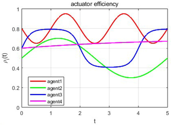
Figure 1. Variation of actuator performance over time in Example 1.

Figure 2 shows the control input signals $u_1\left(t\right)$ and $u_2\left(t\right)$ experiencing severe fluctuations during the attack, indicating that the system cannot receive normal control signals under a DoS attack, leading to abnormal system responses. However, it can also be observed that after the attack ends, the control signals gradually stabilize, suggesting that the control strategy proposed in this paper allows the system to recover to its normal state.

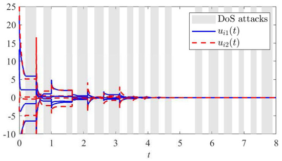
Figure 2. The trajectory of controller (3) over time in Example 1.

According to Theorem 1, when the agents are not under a DoS attack, the control gain of the controller is $k_1$ = 6.4137, and when the agents are subjected to a DoS attack, the control gain of the controller is $k_2$ = 8.2516. The response characteristics of the boundary controller at different time points are shown in Figure 2.

Remark 8.

Under normal conditions, agents continuously adjust their state by processing valid inputs. When a DoS attack occurs, information transmission is blocked. Agents can only rely on the last successfully transmitted value. This value is stored in the buffer. During the attack, agents maintain this value until the next successful transmission. This paper proposes a scheme that allows flexible adjustment of the buffer size, with the agent always operating based on the most recent valid data stored in the buffer.

Figure 3 illustrates the variation in error among the agents in this FOMAS without a controller. The color gradient (blue-green-yellow) represents a continuous increase in values. Over time, the error continues to increase. This indicates that without an effective control mechanism, the system cannot maintain consistency, and the error keeps accumulating over time. Figure 4 demonstrates the variation in the error between the agents in this FOMAS when controller (3) is applied. Although there are some fluctuations in the initial phase, the error gradually stabilizes over time and eventually achieves consistency, effectively controlling the error between the agents. This demonstrates the effectiveness of the control method proposed in this paper.

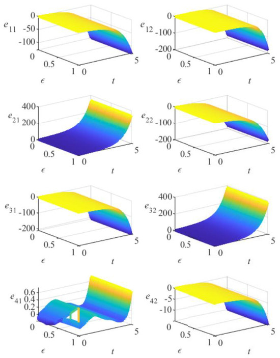
Figure 3. The variation of the error $\epsilon (x,t)$ without a controller in Example 1.

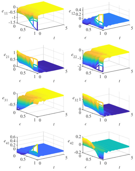
Figure 4. The variation of error $\epsilon (x,t)$ under controller (3) in Example 1.

Example 2.

The verification of Theorem 2 is achieved by introducing a leader-following FOMAS consisting of four agents with the following characteristics: $\underline{\rho }=diag\left([0.35,0.35,0.35,0.35]\right), L=1, n=2, i\in \{1,2,3,4\}, \tau =0.95, f\left(z(x,t)\right)=tanh\left(z(x,t)\right),{\beta }_1=5.6, \widetilde{{\beta }_1}=1.3, {\beta }_2=12, \widetilde{{\beta }_2}=9.7, \sigma =4.0, l_1=3.4, l_2=4.2, \Omega =\left[\begin{array}{cc}4& 0\\ 0& 4\end{array}\right], A=\left[\begin{array}{cc}1.3& -0.5\\ 1& 2.4\end{array}\right]$, and the initial conditions are as follows:

$$\begin{array}{cc}\hfill z_1^0\left(x\right)& ={\left[\begin{array}{c}0.55arctan\left(0.3\pi x\right)-1.4,-0.45e^{0.4x}-1.6\end{array}\right]}^T,\hfill \\ \hfill z_2^0\left(x\right)& ={\left[\begin{array}{c}0.5e^{0.3x},0.3log(1+x^2)-0.95\end{array}\right]}^T,\hfill \\ \hfill z_3^0\left(x\right)& ={\left[\begin{array}{c}0.35(x^2-0.5x),\sqrt{|x+0.2|}+0.65\end{array}\right]}^T,\hfill \\ \hfill z_4^0\left(x\right)& ={\left[\begin{array}{c}0.75tanh\left(0.5\pi x\right)-1.3,log(1+|x\left|\right)-0.8\end{array}\right]}^T,\hfill \end{array}$$

and the actuator efficiency coefficient is:

$$\begin{array}{cc}\hfill {\rho }_1\left(t\right)& =0.85-0.2(1+cos{\displaystyle \frac{\pi t}{4}}),\hfill \\ \hfill {\rho }_2\left(t\right)& =0.6+0.2sin\left({\displaystyle \frac{2\pi t}{3}}\right),\hfill \\ \hfill {\rho }_3\left(t\right)& =0.5+{\displaystyle \frac{0.5}{1+e^{-1.4cos(t-2.5)}}},\hfill \\ \hfill {\rho }_4\left(t\right)& =0.8-0.3e^{-{\displaystyle \frac{t}{2}}}.\hfill \end{array}$$

Figure 5 shows the variation in actuator efficiency over time for four agents in different time periods. Each agent’s efficiency curve exhibits different fluctuations, reflecting the dynamic changes in actuator performance. By introducing actuator efficiency, we can simulate the stability challenges that the system may face in real-world applications due to actuator faults or performance degradation.

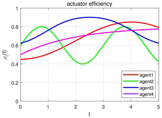
Figure 5. Variation of actuator performance over time in Example 2.

Figure 6 shows the control input signals $u_1\left(t\right)$ and $u_2\left(t\right)$ experiencing severe fluctuations during the attack, indicating that the system cannot receive normal control signals under a DoS attack, leading to abnormal system responses. However, it can also be observed that after the attack ends, the control signals gradually stabilize, suggesting that the control strategy proposed in this paper allows the system to recover to its normal state.

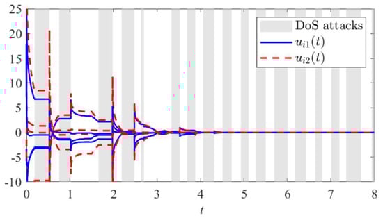
Figure 6. The trajectory of controller (19) over time in Example 2.

According to Theorem 2, when the agents are not under a DoS attack, the control gain of the controller is $k_1$ = 8.3129, and when the agents are subjected to a DoS attack, the control gain of the controller is $k_2$ = 9.8362. The response characteristics of the boundary controller at different time points are shown in Figure 6.

Figure 7 illustrates the variation in error among the agents in this FOMAS without a controller. The color gradient (blue-green-yellow) represents a continuous increase in values. Over time, the error continues to increase. This indicates that without an effective control mechanism, the system cannot maintain consistency, and the error keeps accumulating over time. Figure 8 demonstrates the variation in the error between the agents in this FOMAS when controller (19) is applied. Although there are some fluctuations in the initial phase, the error gradually stabilizes over time and eventually achieves consistency, effectively controlling the error between the agents. This demonstrates the effectiveness of the control method proposed in this paper.

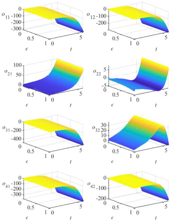
Figure 7. The variation of the error o(x,t) without a controller in Example 2.

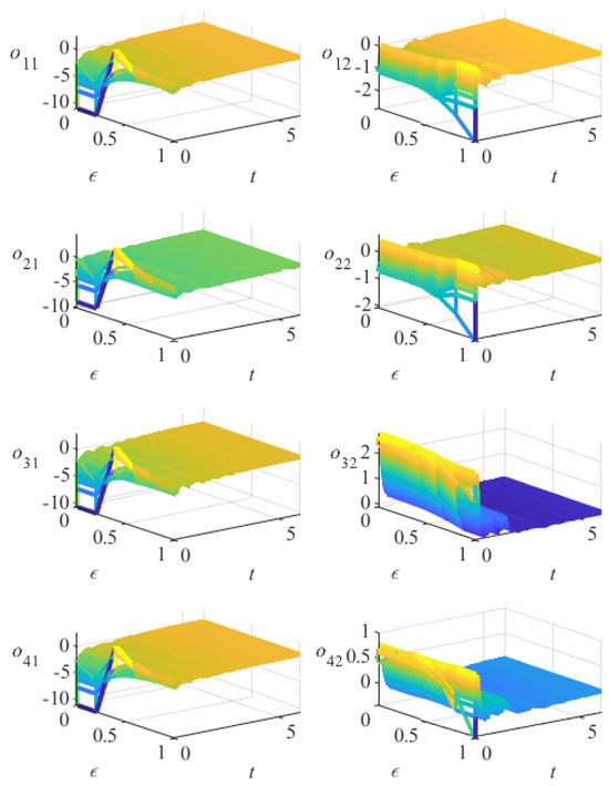
Figure 8. The variation of error $o(x,t)$ under controller (19) in Example 2.

6. Conclusions

This paper has investigated the consensus problem of FOMASs under DoS attacks and actuator faults and has proposed a new approach that applies boundary control strategies to address this issue. The controller relies solely on boundary measurements, thereby significantly reducing its dependence on internal sensors and actuators, as well as control complexity and communication overhead. To prevent communication interruption caused by DoS attacks, a buffering system is incorporated: during DoS attacks, it saves the last correct control input and reinstates it upon recovery, helping to prevent stability loss and consensus breakage and minimizing performance degradation and divergence danger. In addition, actuator efficiency parameters are integrated into the controller structure to allow robust performance despite varying efficiency. Future works shall extend this method to more complex settings, including time-delay networks, heterogeneous agent systems, and event-triggered communication, in an effort to further extend the applicability of the methodology to large-scale distributed intelligent systems.

References

- Zeng, Q.; Nait-Abdesselam, F. Multi-Agent Reinforcement Learning-Based Extended Boid Modeling for Drone Swarms. In Proceedings of the ICC 2024—IEEE International Conference on Communications, Denver, CO, USA, 9–13 June 2024; pp. 1551–1556. [Google Scholar] [CrossRef]
- Yang, Y.; Xiao, Y.; Li, T. Attacks on Formation Control for Multiagent Systems. IEEE Trans. Cybern. 2022, 52, 12805–12817. [Google Scholar] [CrossRef]
- Antonio, G.P.; Maria-Dolores, C. Multi-Agent Deep Reinforcement Learning to Manage Connected Autonomous Vehicles at Tomorrow’s Intersections. IEEE Trans. Veh. Technol. 2022, 71, 7033–7043. [Google Scholar] [CrossRef]
- Xu, R.; Chen, C.J.; Tu, Z.; Yang, M.H. V2X-ViTv2: Improved Vision Transformers for Vehicle-to-Everything Cooperative Perception. IEEE Trans. Pattern Anal. Mach. Intell. 2025, 47, 650–662. [Google Scholar] [CrossRef] [PubMed]
- Wang, T.; Cao, J.; Hussain, A. Adaptive Traffic Signal Control for large-scale scenario with Cooperative Group-based Multi-agent reinforcement learning. Transp. Res. Part C Emerg. Technol. 2021, 125, 103046. [Google Scholar] [CrossRef]
- Zeynivand, A.; Javadpour, A.; Bolouki, S.; Sangaiah, A.; Ja’fari, F.; Pinto, P.; Zhang, W. Traffic flow control using multi-agent reinforcement learning. J. Netw. Comput. Appl. 2022, 207, 103497. [Google Scholar] [CrossRef]
- Liu, G.P. Coordination of Networked Nonlinear Multi-Agents Using a High-Order Fully Actuated Predictive Control Strategy. IEEE/CAA J. Autom. Sin. 2022, 9, 615–623. [Google Scholar] [CrossRef]
- Li, X.; Jiang, H.; Yu, Z.; Ren, Y.; Shi, T.; Chen, S. Leader-following scaled consensus of multi-agent systems based on nonlinear parabolic PDEs via dynamic event-triggered boundary control. Inf. Sci. 2025, 719, 122449. [Google Scholar] [CrossRef]
- Qiu, H.; Korovin, I.; Liu, H.; Gorbachev, S.; Gorbacheva, N.; Cao, J. Distributed adaptive neural network consensus control of fractional-order multi-agent systems with unknown control directions. Inf. Sci. 2024, 655, 119871. [Google Scholar] [CrossRef]
- Li, H.; Liu, S.; Meng, G.; Fan, Q. Dynamic Observer-Based H-Infinity Consensus Control of Fractional-Order Multi-Agent Systems. IEEE Trans. Autom. Sci. Eng. 2025, 22, 12720–12729. [Google Scholar] [CrossRef]
- Zamani, H.; Khandani, K.; Majd, V.J. Fixed-time sliding-mode distributed consensus and formation control of disturbed fractional-order multi-agent systems. ISA Trans. 2023, 138, 37–48. [Google Scholar] [CrossRef]
- Chen, Y.; Shao, S. Discrete-Time Fractional-Order Sliding Mode Attitude Control of Multi-Spacecraft Systems Based on the Fully Actuated System Approach. Fractal Fract. 2025, 9, 435. [Google Scholar] [CrossRef]
- Liu, Y.; Zhang, H.; Shi, Z.; Gao, Z. Neural-Network-Based Finite-Time Bipartite Containment Control for Fractional-Order Multi-Agent Systems. IEEE Trans. Neural Netw. Learn. Syst. 2023, 34, 7418–7429. [Google Scholar] [CrossRef]
- Zhang, X.; Zheng, S.; Ahn, C.K.; Xie, Y. Adaptive Neural Consensus for Fractional-Order Multi-Agent Systems With Faults and Delays. IEEE Trans. Neural Netw. Learn. Syst. 2023, 34, 7873–7886. [Google Scholar] [CrossRef] [PubMed]
- Liu, Y.; Zhang, H.; Wang, Y.; Liang, H. Adaptive Containment Control for Fractional-Order Nonlinear Multi-Agent Systems With Time-Varying Parameters. IEEE CAA J. Autom. Sin. 2022, 9, 1627–1638. [Google Scholar] [CrossRef]
- Zhong, Y.; Yuan, Y.; Yuan, H. Nash Equilibrium Seeking for Multi-Agent Systems Under DoS Attacks and Disturbances. IEEE Trans. Ind. Inform. 2024, 20, 5395–5405. [Google Scholar] [CrossRef]
- Xu, H.; Zhu, F.; Ling, X. Secure bipartite consensus of leader–follower multi-agent systems under denial-of-service attacks via observer-based dynamic event-triggered control. Neurocomputing 2025, 614, 128817. [Google Scholar] [CrossRef]
- Wen, H.; Li, Y.; Tong, S. Distributed adaptive resilient formation control for nonlinear multi-agent systems under DoS attacks. Sci. China Inf. Sci. 2024, 67, 209201. [Google Scholar] [CrossRef]
- Liu, J.; Dong, Y.; Gu, Z.; Xie, X.; Tian, E. Security consensus control for multi-agent systems under DoS attacks via reinforcement learning method. J. Frankl. Inst. 2024, 361, 164–176. [Google Scholar] [CrossRef]
- Chen, P.; Liu, S.; Chen, B.; Yu, L. Multi-Agent Reinforcement Learning for Decentralized Resilient Secondary Control of Energy Storage Systems Against DoS Attacks. IEEE Trans. Smart Grid 2022, 13, 1739–1750. [Google Scholar] [CrossRef]
- Zhao, N.; Zhang, H.; Shi, P. Observer-Based Sampled-Data Adaptive Tracking Control for Heterogeneous Nonlinear Multi-Agent Systems Under Denial-of-Service Attacks. IEEE Trans. Autom. Sci. Eng. 2025, 22, 4771–4779. [Google Scholar] [CrossRef]
- Zhao, Y.; Sun, H.; Yang, J.; Hou, L.; Yang, D. Event-Triggered Fully Distributed Bipartite Containment Control for Multi-Agent Systems Under DoS Attacks and External Disturbances. IEEE Trans. Circuits Syst. I Regul. Pap. 2025, 72, 6011–6024. [Google Scholar] [CrossRef]
- Wang, J.; Yan, Y.; Liu, Z.; Chen, C.P.; Zhang, C.; Chen, K. Finite-time consensus control for multi-agent systems with full-state constraints and actuator failures. Neural Netw. 2023, 157, 350–363. [Google Scholar] [CrossRef] [PubMed]
- Zhang, Y.; Li, H.; Sun, J.; He, W. Cooperative Adaptive Event-Triggered Control for Multiagent Systems With Actuator Failures. IEEE Trans. Syst. Man Cybern. Syst. 2019, 49, 1759–1768. [Google Scholar] [CrossRef]
- Deng, C.; Gao, W.; Che, W. Distributed adaptive fault-tolerant output regulation of heterogeneous multi-agent systems with coupling uncertainties and actuator faults. IEEE CAA J. Autom. Sin. 2020, 7, 1098–1106. [Google Scholar] [CrossRef]
- Li, J.; Yan, Z.; Shi, X.; Luo, X. Distributed Adaptive Formation Control for Fractional-Order Multi-Agent Systems with Actuator Failures and Switching Topologies. Fractal Fract. 2024, 8, 563. [Google Scholar] [CrossRef]
- Zhang, T.; Lin, M.; Xia, X.; Yi, Y. Adaptive cooperative dynamic surface control of non-strict feedback multi-agent systems with input dead-zones and actuator failures. Neurocomputing 2021, 442, 48–63. [Google Scholar] [CrossRef]
- Zhang, Z.; Dong, J. Containment control of interval type-2 fuzzy multi-agent systems with multiple intermittent packet dropouts and actuator failure. J. Frankl. Inst. 2020, 357, 6096–6120. [Google Scholar] [CrossRef]
- Lui, D.G.; Petrillo, A.; Santini, S. Adaptive fault-tolerant containment control for heterogeneous uncertain nonlinear multi-agent systems under actuator faults. J. Frankl. Inst. 2024, 361, 107317. [Google Scholar] [CrossRef]
- Su, Y.; Shan, Q.; Liang, H.; Li, T.; Zhang, H. Event-Based Adaptive Optimal Fault-Tolerant Consensus Control for Uncertain Nonlinear Multiagent Systems With Actuator Failures. IEEE Trans. Syst. Man Cybern. Syst. 2025, 55, 7273–7287. [Google Scholar] [CrossRef]
- Long, S.; Huang, W.; Wang, J.; Liu, J.; Gu, Y.; Wang, Z. A Fixed-Time Consensus Control With Prescribed Performance for Multi-Agent Systems Under Full-State Constraints. IEEE Trans. Autom. Sci. Eng. 2025, 22, 6398–6407. [Google Scholar] [CrossRef]
- Jiang, Y.; Liu, L.; Feng, G. Fully distributed adaptive control for output consensus of uncertain discrete-time linear multi-agent systems. Automatica 2024, 162, 111531. [Google Scholar] [CrossRef]
- Xu, N.; Chen, Z.; Niu, B.; Zhao, X. Event-Triggered Distributed Consensus Tracking for Nonlinear Multi-Agent Systems: A Minimal Approximation Approach. IEEE J. Emerg. Sel. Top. Circuits Syst. 2023, 13, 767–779. [Google Scholar] [CrossRef]
- Hu, W.; Cheng, Y.; Yang, C. Leader-following consensus of linear multi-agent systems via reset control: A time-varying systems approach. Automatica 2023, 149, 110824. [Google Scholar] [CrossRef]
- Song, X.; Sun, X.; Song, S.; Zhang, Y. Secure Consensus Control for PDE-Based Multiagent Systems Resist Hybrid Attacks. IEEE Syst. J. 2023, 17, 3047–3058. [Google Scholar] [CrossRef]
- Liu, Y.; Zuo, Z.; Song, J.; Li, W. Fixed-time consensus control of general linear multiagent systems. IEEE Trans. Autom. Control 2024, 69, 5516–5523. [Google Scholar] [CrossRef]
- Peng, X.J.; He, Y.; Li, H.; Tian, S. Consensus Control and Optimization of Time-Delayed Multiagent Systems: Analysis on Different Order-Reduction Methods. IEEE Trans. Syst. Man Cybern. Syst. 2025, 55, 780–791. [Google Scholar] [CrossRef]
- Hao, Y.; Fang, Z.; Cao, J.; Liu, H. Consensus Control of Nonlinear Fractional-Order Multiagent Systems With Input Saturation: A T–S Fuzzy Method. IEEE Trans. Fuzzy Syst. 2024, 32, 6754–6766. [Google Scholar] [CrossRef]
- Seuret, A.; Gouaisbaut, F. Wirtinger-based integral inequality: Application to time-delay systems. Automatica 2013, 49, 2860–2866. [Google Scholar] [CrossRef]
- Qin, J.; Gao, H.; Zheng, W.X. Exponential Synchronization of Complex Networks of Linear Systems and Nonlinear Oscillators: A Unified Analysis. IEEE Trans. Neural Netw. Learn. Syst. 2015, 26, 510–521. [Google Scholar] [CrossRef]
- Lv, Y.; Hu, C.; Yu, J.; Jiang, H.; Huang, T. Edge-Based Fractional-Order Adaptive Strategies for Synchronization of Fractional-Order Coupled Networks With Reaction–Diffusion Terms. IEEE Trans. Cybern. 2020, 50, 1582–1594. [Google Scholar] [CrossRef]
- Li, Y.; Chen, Y.; Podlubny, I. Mittag–Leffler stability of fractional order nonlinear dynamic systems. Automatica 2009, 45, 1965–1969. [Google Scholar] [CrossRef]
- Yang, C.; Huang, T.; Yi, K.; Zhang, A.; Chen, X.; Li, Z.; Qiu, J.; Alsaadi, F.E. Synchronization for nonlinear complex spatio-temporal networks with multiple time-invariant delays and multiple time-varying delays. Neural Process. Lett. 2019, 50, 1051–1064. [Google Scholar] [CrossRef]
- Liu, C.; Wang, W.; Jiang, B.; Patton, R.J. Fault-Tolerant Consensus of Multi-Agent Systems Subject to Multiple Faults and Random Attacks. IEEE Trans. Circuits Syst. I Regul. Pap. 2025, 72, 4935–4945. [Google Scholar] [CrossRef]
- Chen, J.; Shen, J.; Chen, W.; Li, J.; Zhang, S. Application of Robust Fuzzy Cooperative Strategy in Global Consensus of Stochastic Multi-Agent Systems. IEEE Trans. Autom. Sci. Eng. 2025, 22, 12058–12070. [Google Scholar] [CrossRef]
- De Persis, C.; Tesi, P. Input-to-State Stabilizing Control Under Denial-of-Service. IEEE Trans. Autom. Control 2015, 60, 2930–2944. [Google Scholar] [CrossRef]
- Yan, L.; Liu, Z.; Philip Chen, C.; Zhang, Y.; Wu, Z. Optimized adaptive consensus control for multi-agent systems with prescribed performance. Inf. Sci. 2022, 613, 649–666. [Google Scholar] [CrossRef]
- Sun, Y.; Shi, P.; Lim, C.C. Event-triggered sliding mode scaled consensus control for multi-agent systems. J. Frankl. Inst. 2022, 359, 981–998. [Google Scholar] [CrossRef]
Disclaimer/Publisher’s Note: The statements, opinions and data contained in all publications are solely those of the individual author(s) and contributor(s) and not of MDPI and/or the editor(s). MDPI and/or the editor(s) disclaim responsibility for any injury to people or property resulting from any ideas, methods, instructions or products referred to in the content. |
© 2025 by the authors. Licensee MDPI, Basel, Switzerland. This article is an open access article distributed under the terms and conditions of the Creative Commons Attribution (CC BY) license (https://creativecommons.org/licenses/by/4.0/).