Season-Resolved, Fluctuation-Level Regional Connectivity of PM_2.5 over the Korean Peninsula Revealed by Multifractal Detrended Cross-Correlation Networks (2016–2020)

Abstract

Motivated by the strong seasonality of East Asian meteorology and its control on pollution episodes characterized by fluctuation level, we model the season-resolved climatology of the regional PM_2.5 connectivity over the Korean Peninsula. Using daily AirKorea data for 2016–2020, we (i) remove daily climatology and the peninsula-wide background (empirical orthogonal function; EOF1) to obtain residual signals; (ii) compute the sign-preserving multifractal detrended cross-correlation coefficient MFDCCA-$\rho \left(q,s\right)$; (iii) apply iAAFT surrogate significance across scales; and (iv) construct signed, weighted networks aggregated over short (5–15 d) and mid (15–30 d) bands for DJF/MAM/JJA/SON. Our analysis targets the seasonal climatology of fluctuation-level ($q$-dependent) connectivity by pooling seasons across years; this approach increases statistical robustness at 5–30-day scales and avoids diluting season-specific organization. We find negligible connectivity for $q<0$ (small fluctuations) but dense, seasonally organized networks for $q>0$ (strongest in winter–spring and at 15–30 days). After removing the EOF1, positive subgraphs form assortative regional backbones, while negative subgraphs reveal a northwest–southeast anti-phase dipole; the connectivity around Baengnyeongdo (B) highlights a transboundary sentinel role in cool seasons. These results demonstrate that a season-resolved, fluctuation-level framework effectively isolates regional connectivity that would otherwise be masked in annual aggregates or by the peninsula-wide background.

1. Introduction

Air pollution is the contamination of the indoor or outdoor environment by any chemical, physical, or biological processes modifying the natural characteristics of the atmosphere. Pollutants of major public health concern include particulate matter, carbon monoxide, ozone, nitrogen dioxide, and sulfur dioxide. Among those pollutants, fine particulate matter (PM_2.5) is a leading environmental risk factor; epidemiology links exposure to cardiopulmonary outcomes and a reduced life expectancy [1].

The source of PM may be either direct emissions into the air or conversion from gaseous precursors released from both anthropogenic and natural sources. Anthropogenic sources are highly variable with a wide range of temporal scales and include solid fuel combustion, industrial and agricultural activities, and vehicular emissions, such as the erosion of the pavement and the abrasion of brakes and tires [2,3], while natural sources include volcanoes, dust storms, forest fires, living vegetation, and sea spray [4]. PM exhibits different lifetimes and transport distances according to size; smaller particles can remain suspended for days to weeks and be transported for hundreds of kilometers [5,6]. PM_2.5 therefore persists long enough to enable synoptic-scale advection and long-range transport that shape spatiotemporal patterns of episodes.

Among factors affecting local PM concentrations, meteorological parameters play a significant role in dispersion, transformation, and removal [7]. Previous studies show that PM concentrations are strongly modulated by regional meteorology [8,9,10].

South Korea is located downwind of China, Mongolia, and Russia, and the PM variability is strongly influenced by long-range transport and synoptic conditions. Prior studies over Korea report sizable transboundary contributions that vary with the season and meteorological regime [11,12,13,14]. Yim et al. (2019) found that the impact of transboundary emissions from China on South Korea’s air quality was nearly 70%, with a 30% contribution from local emissions [15]; during extreme pollution periods, Chinese and domestic contributions reached 68% and 26%, respectively [16], whereas during blocking conditions the situation reversed, with 25% from China and 57% from local sources [15,16]. These findings underscore the seasonal and synoptic control of PM over the peninsula.

PM concentrations also display multifractal variability [17], with large-amplitude bursts (episodes) and small-amplitude background fluctuations reflecting different processes and couplings. A detrended cross-correlation analysis (DCCA) quantifies scale-specific correlations under nonstationarity [18], and its multifractal extensions (MFDCCA and MFCCA) introduce a $q$-dependent emphasis on small or large fluctuations [19,20]. Accordingly, a fluctuation-level, scale-resolved, and cross-correlation framework is well-suited to probe the regional PM_2.5 connectivity over Korea.

A central aim of this study is to quantify the seasonal climatology of the regional PM_2.5 connectivity over the Korean Peninsula in terms of the fluctuation level. We therefore adopt a season-resolved (DJF/MAM/JJA/SON) design to (i) preserve the season-specific organization linked to East Asian monsoon regimes, (ii) avoid the dilution that occurs when annual aggregates blur seasonal structures, and (iii) ensure robust sample lengths at 5–30-day scales under missing data constraints. To this end, we analyze 2016–2020 daily AirKorea data, remove the daily climatology and the leading EOF mode to obtain residual signals, compute the sign-preserving MFDCCA- $\rho \left(q,s\right)$, and—after iAAFT surrogate significance testing [21]—build signed (positive/negative) networks aggregated over 5–15-day and 15–30-day bands. Methodological details are provided in Section 2.

The contributions are threefold: (i) a fluctuation-level lens that separates small- vs. large-amplitude covariability in the regional PM_2.5; (ii) a signed graph decomposition that distinguishes in-phase regional backbones (positive) from northwest (NW)–southeast (SE) anti-phase couplings (negative); and (iii) a seasonal, scale-resolved characterization consistent with the meteorological organization over Korea.

This paper is organized as follows. In the following data and methodology section, we provide a brief description of the PM_2.5 dataset along with its preprocessing procedure and introduce the analysis methods. Analysis results as well as their interpretations are presented in the result section, and the last section contains the implication of our results and cautionary comments.

2. Materials and Methods

2.1. Data Sampling and Processing

We use daily PM_2.5 signals covering 2016–2020 (1827 days) from the Korean Ministry of Environment (KMOE)/AirKorea monitoring network [22]. Station selection requires ≤100 missing days over the full period to ensure reliable seasonal coverage. Hourly records are aggregated to daily means following standard quality control procedures. Missing values are handled in two steps: (i) linear interpolation for short gaps up to 7 consecutive days and (ii) omission of longer gaps so that only overlapping, quality-controlled data enter the pairwise calculations.

Seasonal time series are constructed by a cut-and-stitch approach that concatenates, for each season (DJF/MAM/JJA/SON), all corresponding segments across 2016–2020. After removing the daily climatology to suppress the seasonal cycle, we estimate and subtract the leading empirical orthogonal function (EOF1) from the space–time matrix of anomalies to obtain residual signals that down-weight the peninsula-wide background (details in Section 2.2.2). We then compute the sign-preserving multifractal cross-correlation coefficient MFDCCA-$\rho \left(q,s\right)$ on the residuals for window size $s\in \left[5, 30\right]$ days and aggregate $\rho$ over two scale bands: short (5–15 day) and mid (15–30 day).

2.2. Methodology

2.2.1. Daily Climatology Detrending

Let $x_i\left(t\right)$ be the daily mean PM_2.5 at station $i$ on day $t$ ($t=1\dots , T$). Denote DOY by $d\left(t\right)\in \left\{1,\dots , 365\right\}$ (leap day omitted or reassigned; here, reassigned). The daily climatology is

$${\overline{x}}_i\left(d\right)={\displaystyle \frac{1}{\left|{\mathrm{T}}_d\right|}}{\displaystyle \sum }_{t\in {\mathrm{T}}_d}{x}_i\left(t\right) ,$$

(1)

where ${\mathrm{T}}_d$ denotes the set of years to be considered in this study, that is, 2016–2020. Then, the de-climatized anomaly is

$${x\prime }_i\left(t\right)=x_i\left(t\right)-{\overline{x}}_i\left(d\left(t\right)\right).$$

(2)

For missing values, we used interpolation or omission, with a maximum gap length consistent with our preprocessing; extremely long NaN windows (in this study, $>7d$) are left missing and excluded from pairwise computations.

2.2.2. Removing the Wide Effect (EOF1 Residuals)

Stack the de-climatized series as a matrix $X\prime \in {ℝ}^{T\times N}$ (time $\times$ stations), standardized column-wise. Compute the SVD, $X\prime =U\Sigma V^{\mathrm{T}}$. The first principal component (PC1) and loading are $p_1=U_{:,1}{\sigma }_1$ and $v_1=V_{:,1}$. We remove the rank-1 part $X_1=p_1{v}_1^{\mathrm{T}}$ and define the residual (regional) signals

$$X_{\mathrm{res}}=X\prime -X_1.$$

(3)

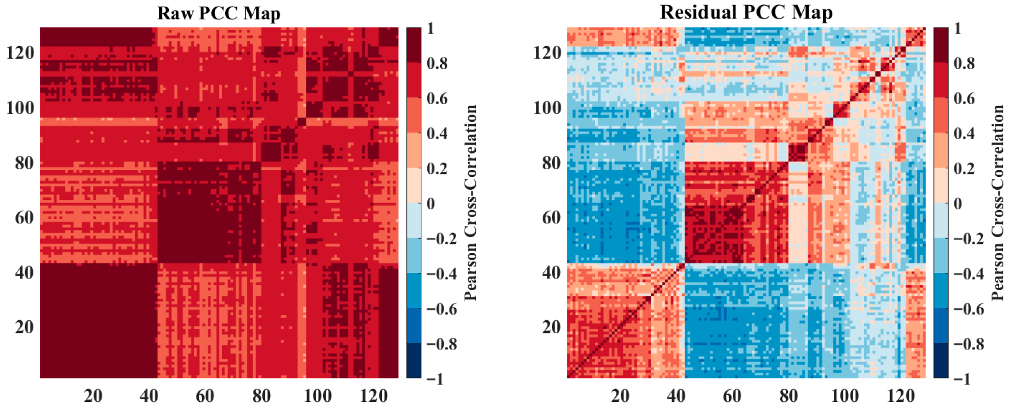
This step removes the peninsula-wide background. For clarity, we compared Pearson cross-correlations computed on the original daily anomalies ($X\prime$) and on the EOF1-removed residuals (Figure A1). The original series show widespread positive correlations, whereas after removing EOF1, the regional structure—including negative NW-SE pairs—emerges much more clearly. This confirms that EOF1 plays the role in the peninsula-wide background, and its removal enhances the visibility of regional connectivity in the subsequent network analysis.

2.2.3. Multifractal Detrended Cross-Correlation Analysis (MFDCCA) and $\rho \left(q,s\right)$

For two residual series, $x\left(t\right) \mathrm{and} y\left(t\right),$ we form the cumulative profiles

$$X\left(k\right)={\displaystyle \sum }_{t=1}^k\left[x\left(t\right)-x\right] ,\hspace{1em} Y\left(k\right)={\displaystyle \sum }_{t=1}^k\left[y\left(t\right)-y\right]$$

(4)

where $\langle ·\rangle$ denotes the temporal mean. For a box size $s$ (here, $5\le s\le 30$ days), partition each profile into $N_s=\mathrm{int}\left(N/s\right)$ non-overlapping segments from the beginning and $N_s$ from the end (total 2 $N_s$ segments). In each $\nu$ segment, remove a local polynomial trend of order $m$ (we use $m=1$) from both profiles, producing ${\tilde{X}}_{\nu }^{\left(m\right)}\left(k\right)$ and ${\tilde{Y}}_{\nu }^{\left(m\right)}\left(k\right)$. The detrended covariance in segment $\nu$ is

$$F_{XY}^2\left(\nu ,s\right)={\displaystyle \frac{1}{s}}{\displaystyle \sum }_{k=1}^s\left\{\left(X\left[\left(\nu -1\right)s+k\right]-{\tilde{X}}_{\nu }^{\left(m\right)}\left(k\right)\right)\times \left(Y\left[\left(\nu -1\right)s+k\right]-{\tilde{Y}}_{\nu }^{\left(m\right)}\left(k\right)\right)\right\}$$

(5)

The corresponding variances are given as $F_{XX}^2\left(\nu ,s\right)$ and $F_{YY}^2\left(\nu ,s\right)$, respectively. Then, $q$-order fluctuation functions are

$$\begin{gathered} F_{XY}\left(q,s\right)={\left[{\displaystyle \frac{1}{2N_s}}{\displaystyle \sum }_{\nu =1}^{2N_s}\mathrm{sgn}\left(F_{XY}^2\left(\nu ,s\right)\right){\left|F_{XY}^2\left(\nu ,s\right)\right|}^{q/2}\right]}^{1/q}, \\ {F}_{XX}\left(q,s\right)={\left[{\displaystyle \frac{1}{2N_s}}{\displaystyle \sum }_{\nu =1}^{2N_s}{\left|F_{XX}^2\left(\nu ,s\right)\right|}^{{\displaystyle \frac{q}{2}}}\right]}^{{\displaystyle \frac{1}{q}}}, \\ {F}_{YY}\left(q,s\right)={\left[{\displaystyle \frac{1}{2N_s}}{\displaystyle \sum }_{\nu =1}^{2N_s}{\left|F_{YY}^2\left(\nu ,s\right)\right|}^{q/2}\right]}^{1/q}. \end{gathered}$$

(6)

These functions are defined for $q\ne 0$, and, in this study, $q=0$ is not considered. Using Equation (6), we define the $q$-dependent, sign-preserving cross-correlation coefficient as

$$\rho \left(q,s\right)={\displaystyle \frac{F_{XY}\left(q,s\right)}{\sqrt{F_{XX}\left(q,s\right)F_{YY}\left(q,s\right)}}}\in \left[-1, 1\right] ,$$

(7)

according to the work of Kwapień et al. (2015) [23]. In this multifractal formalism, positive $q$ emphasizes large fluctuations; negative $q$ emphasizes small fluctuation [24]. The formulation follows MFDCCA/MFCCA and DCCA literature for nonstationary cross-correlations [18,19,20].

We used $q\in \left\{-5,-2, 2, 5\right\}$ and window sizes of $s\in \left[5, 30\right]$ days. For each $\left(i,j\right)$ pair, we aggregate within short (5–15 d) and mid (15–30 d) bands by the mean ${\overline{\rho }}_q^{\mathrm{band}}\left(i,j\right)$ over the included $s$. For every pair, only overlapping days enter a box; segments with insufficient points are skipped.

2.2.4. Significance via iAAFT Surrogates

Since there is no a priori null distribution for $\rho \left(q,s\right)$, we utilize a surrogate-based Monte Carlo framework to compute the critical values for significance testing [25]. For each station $i$, we generated iAAFT surrogates that preserve the empirical amplitude distribution and (approximately) the power spectrum, repeated $N_{sur}=100$ times [21]. For a given pair, we computed $\rho \left(q,s\right)$ on each surrogate pair and derived a sample distribution for the null hypothesis of no cross-correlation beyond linear correlations encapsulated by the surrogates. An empirical two-sided test at $\alpha =0.05$ was applied scale-wise, and a pair was deemed significant for a band if the fraction of significant scales in the band exceeded a pre-determined minimum (herein, 50%).

2.2.5. Signed, Weighted Network Construction

Let $W^{\left(q,\mathrm{band}\right)}=\left[w_{ij}\right]$ with $w_{ij}={\overline{\rho }}_q^{\mathrm{band}}\left(i,j\right)$ if the pair is significant and 0 otherwise. We analyze three types of networks:

• All-edged network (signed): $W$ with both positive and negative weights.
• Positive subgraph: $W_{ij}^{+}=\max \left(w_{ij},0\right)$.
• Negative subgraph: $W_{ij}^{-}=-\min \left(w_{ij},0\right)$ (magnitudes as weights).

When desired for visualization, an additional magnitude threshold $\left|w_{ij}\right|\ge \theta$ (in this study, $\theta =0.5$) can be applied after significance to emphasize the strongest edges. Note that setting $\theta =0$ yields the fully significant network. For all networks in the following figures, edge existence is determined solely by statistical significance (iAAFT). Any subsequent magnitude threshold on $\left|\rho \right|$ (equal to $\left|w_{ij}\right|$) is optional and used for visualization/summarization only; setting the threshold to 0 ($\theta =0$) renders all significant edges.

2.2.6. Global Network Measures

For each network (by season, band, and $q$), we computed the following global descriptors (no node-wise metrics in this study).

(1). 

Edge density: $\delta =2E/\left[N\left(N-1\right)\right]$, with $E$ as the number of nonzero edges. This quantifies the overall connectivity of the PM_2.5 system. A higher density suggests that most monitoring stations exhibit significant cross-correlations with one another, implying a highly interconnected and potentially uniform regional pollution system.

(2). 

Mean absolute weight: $\left|w\right|={\displaystyle \frac{1}{E}}{{\displaystyle \sum }}_{i<j}\left|w_{ij}\right|$. This measure quantifies the average covarying strength among all significant edges. A higher value indicates a high synchronization.

(3). 

Weighted characteristic path length $L_w$: Shortest paths are computed on distances $d_{ij}=1/\left|w_{ij}\right|$ (for connected pairs) then averaged over all node pairs in the largest connected component [26]. This quantifies the global integration/efficiency of a network, implying that a smaller value indicates the closeness of connectivity.

(4). 

Degree assortativity (weighted): Newman’s assortativity is computed on node strengths (weighted degree), as an average correlation of endpoint strengths across edges [27,28], that is, $r_s=\mathrm{corr}\left(s_i,s_j\right), s_i={{\displaystyle \sum }}_{j\ne i}\left|w_{ij}\right|$. Assortativity ($r_s>0$) means nodes with high overall correlation strength tend to connect to other high-strength nodes (that is, major pollution centers synchronize). Disassortativity ($r_s<0)$ means high-strength nodes tend to connect to low-strength nodes (a major source site influences many minor sites).

3. Analysis Results

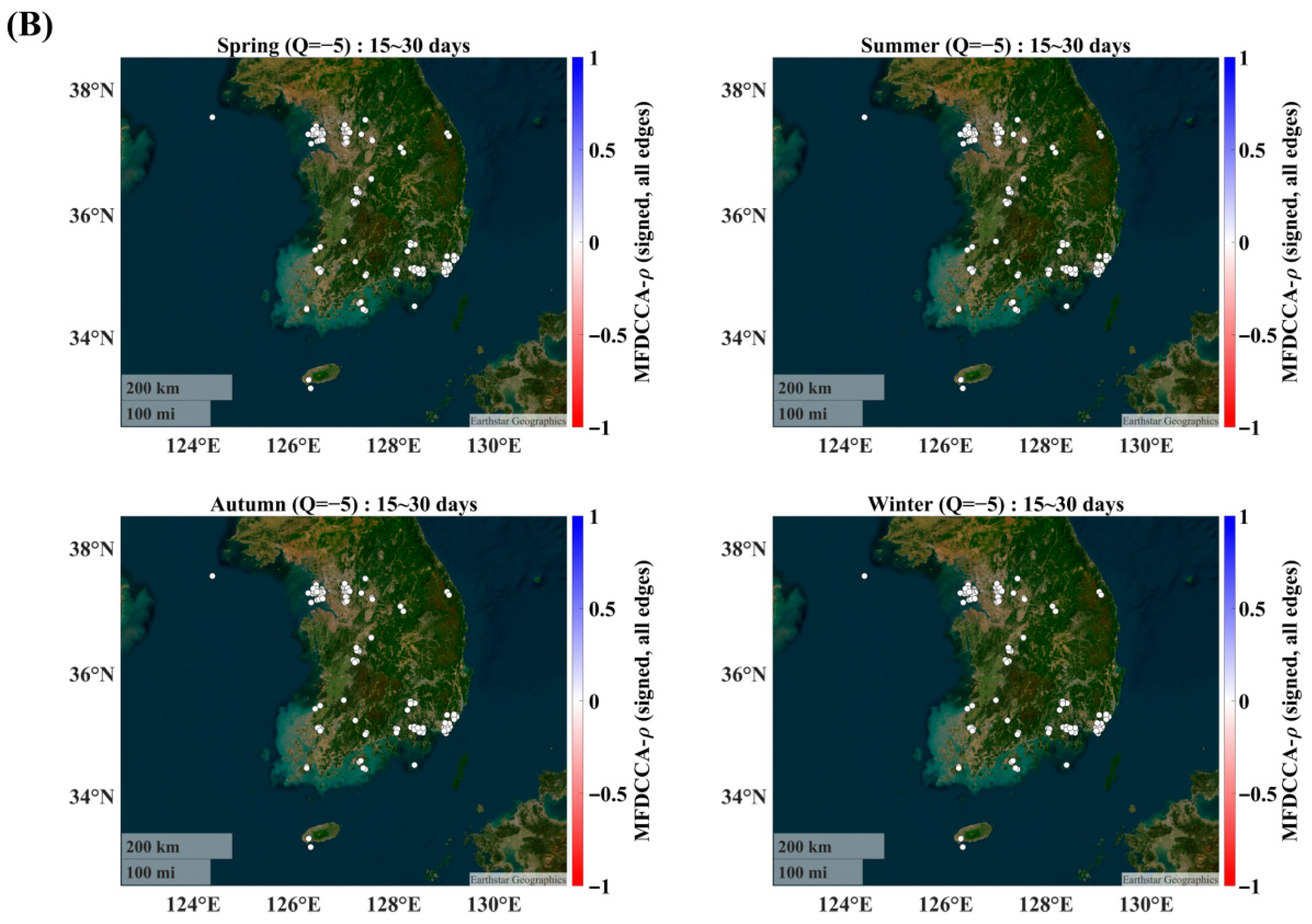
Across seasons and scales, multifractal cross-correlations in daily PM_2.5 residuals (MFDCCA–$\rho$) organize into a dense, largely positive network for $q$ > 0 and an extremely sparse/vanishing network for $q$ < 0 under the significance (iAAFT, $\alpha$ = 0.05) and absolute weight threshold (|$\rho$| ≥ 0.5), as clearly seen in Figure A2. It should be noted that all the network metrics were computed from significantly constructed networks via iAAFT surrogate significant testing. Additionally, for the visuality of positively and negatively connected subgraphs, we apply the absolute weight threshold (|$\rho$| ≥ 0.5) to the significant edge weights. Visually and metrically, the connectivity increases (i) from summer to winter and (ii) from the short band (5–15 days) to the mid band (15–30 days).

A small set of coherent negative edges appears repeatedly and preferentially links the northwest cluster (Seoul–Incheon–Gyeonggi) to southeastern coastal/industrial nodes (Busan–Ulsan–Changwon), consistent with the out-of-phase fluctuations at those locations. The Baengnyeongdo (B) station, positioned along the main corridor of the westerly inflow from China, often emerges as a well-connected hub—especially for $q$ > 0 and in spring–winter—matching the seasonality and geography of the long-range transport to Korea reported in prior work [29,30]. These studies show that westerly and northwesterly regimes in winter and spring, together with stagnant conditions over the peninsula, enhance the imported PM_2.5 and its covariation across Korean sites, with typical transboundary contributions of several tens of percent on polluted days [30].

3.1. Spring (MAM)

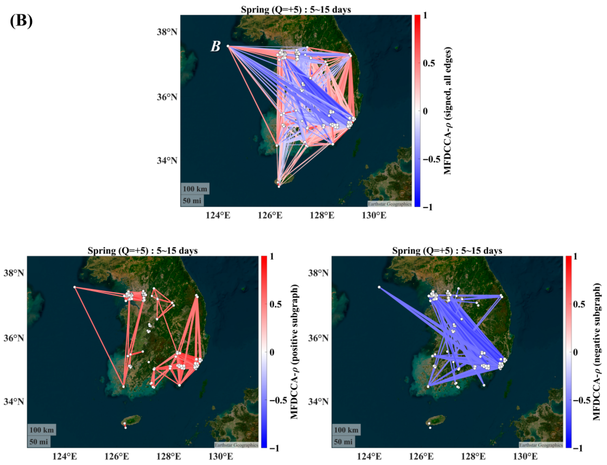
Signed, all-edges view ($\mathit{q}\mathbf{=}\mathbf{+}\mathbf{2} \mathbf{and}\mathbf{+}\mathbf{5}$): In both scale bands (5–15 d and 15–30 d), the spring network is already near-percolated for $q$ > 0, with most stations linked by a positive $\rho$. Increasing the $q$ from +2 to +5 sharpens this picture: edges thicken around the capital area and the central-west corridor, and Baengnyeongdo (B) gains strong ties to western and southwestern mainland sites (Figure 1A,B and Figure 2A,B, top panels). This is fully consistent with springtime westerlies and the well-documented pathway from east-central/northeastern China to Korea, which raises PM_2.5 over the western half of the peninsula and imprints a common, large-fluctuation signal across stations [28].

Positive vs. negative subgraphs ($\mathit{q}\mathbf{=}\mathbf{+}\mathbf{2} \mathbf{and}\mathbf{+}\mathbf{5}$): The positive subgraph (red) forms a coast-to-coast backbone (western coast of Seoul–Incheon–Gyeonggi $\to$ Yeongnam coast), which is more complete at 15–30 d than at 5–15 d (Figure 1A,B and Figure 2A,B, bottom-left and bottom-right panels). The negative subgraph (blue) is sparser and accentuates long links between northwest nodes and the southeast coast, suggesting anti-phased regional variability—plausibly a combination of synoptic passages and land–sea–breeze contrasts that modulate accumulation/ventilation differently across regions. This spatial contrast aligns with analyses showing that meteorology controls both the co-fluctuation and dispersion of PM over Korea, with stronger lateral transport in spring [29].

3.2. Summer (JJA)

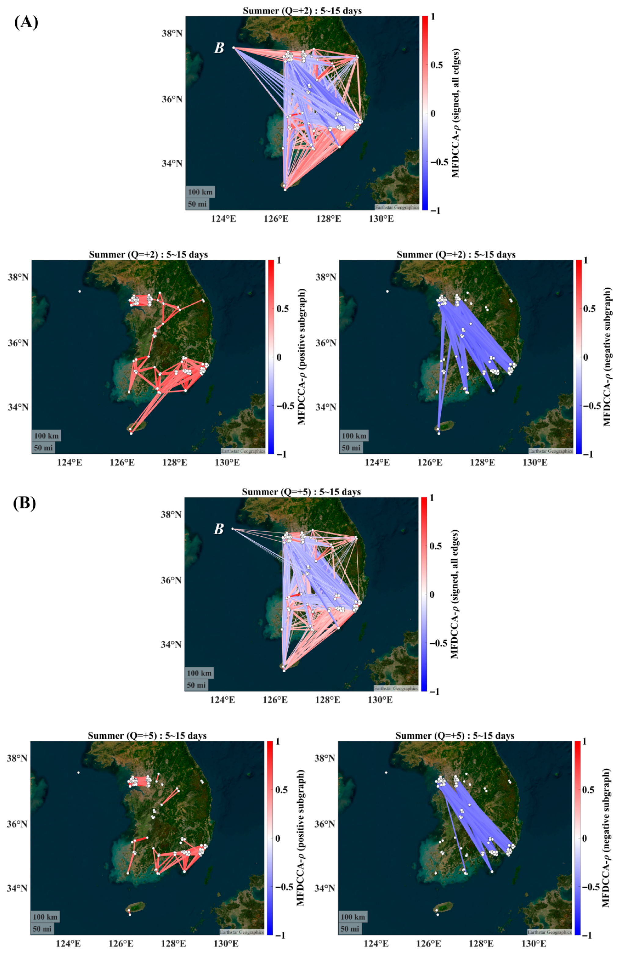
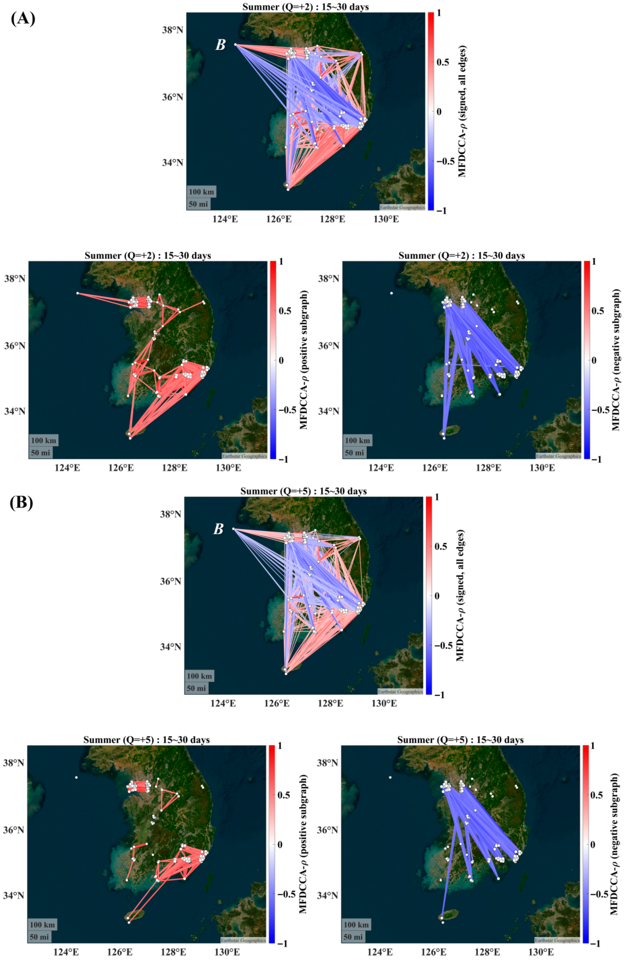
Signed, all-edges view ($\mathit{q}\mathbf{=}+\mathbf{2} \mathbf{and}\mathbf{+}\mathbf{5}$): Summer shows the weakest connectivity among the seasons for the short band (5–15 d)—positive edges still dominate but are thinner and fewer, especially inland (Figure 3A,B, top). Moving to the mid band (15–30 d) partially restores the backbone, though it is still below the spring/winter density (Figure 4A,B, top). This reduction is consistent with enhanced convection, higher humidity, and frequent precipitation, which disrupt the persistence and cross-site co-fluctuation of large PM_2.5 anomalies in summer [29].

Positive vs. negative subgraphs ($\mathit{q}\mathbf{=}\mathbf{+}\mathbf{2} \mathbf{and}\mathbf{+}\mathbf{5}$): The positive subgraph concentrates along coasts and major urban corridors and becomes more fragmented inland at 5–15 d. The negative subgraph is very sparse, dominated by a handful of north–south long edges (Figure 3A,B and Figure 4A,B, bottom). The overall picture matches the reported summer behavior—lower PM_2.5 variability and a weaker transboundary influence—leading to a smaller and less coherent $\rho$ for large fluctuations [29].

3.3. Autumn (SON)

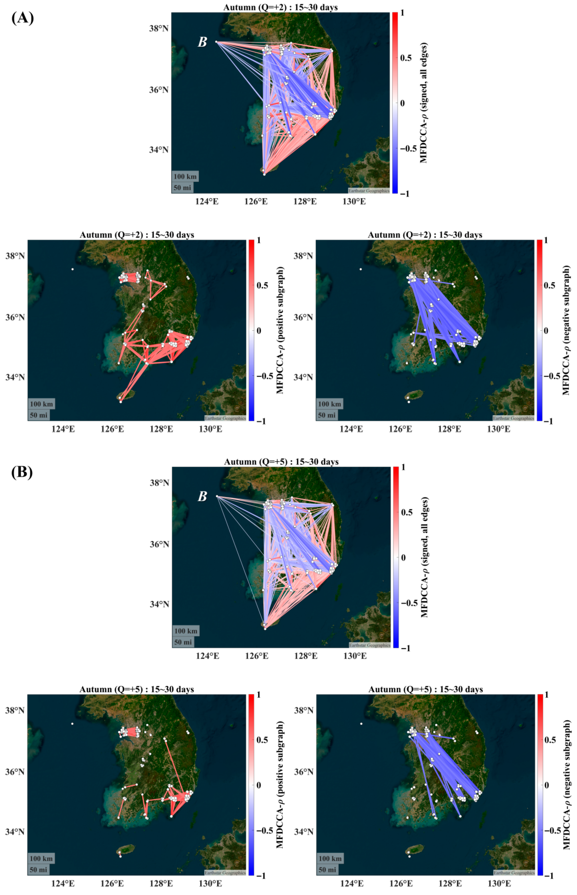
Signed, all-edges view ($\mathit{q}\mathbf{=}\mathbf{+}\mathbf{2} \mathbf{and}\mathbf{+}\mathbf{5}$): Autumn re-strengthens the network relative to summer. For $q>0$, most stations again belong to one giant component, with thicker positive edges along the western corridor and Baengnyeongdo (B) reconnecting strongly as a gateway (Figure 5A,B, top). The 15–30 d maps further intensify these structures (Figure 6A,B, top), indicating more coherent, slowly varying drivers in the fall transition.

Positive vs. negative subgraphs ($\mathit{q}\mathbf{=}\mathbf{+}\mathbf{2} \mathbf{and}\mathbf{+}\mathbf{5}$): As in spring, the positive subgraph at 15–30 d effectively tiles the peninsula. The negative subgraph remains selective—notably northwest $\leftrightarrow$ southeast links—signaling sub-regional out-of-phase episodes even as the overall coherence increases. This is consistent with the climatological shift toward more frequent stagnant/high-pressure situations in the cool season transition, which favors accumulation and shared variability in western Korea while still allowing phase differences across basins [29].

3.4. Winter (DJF)

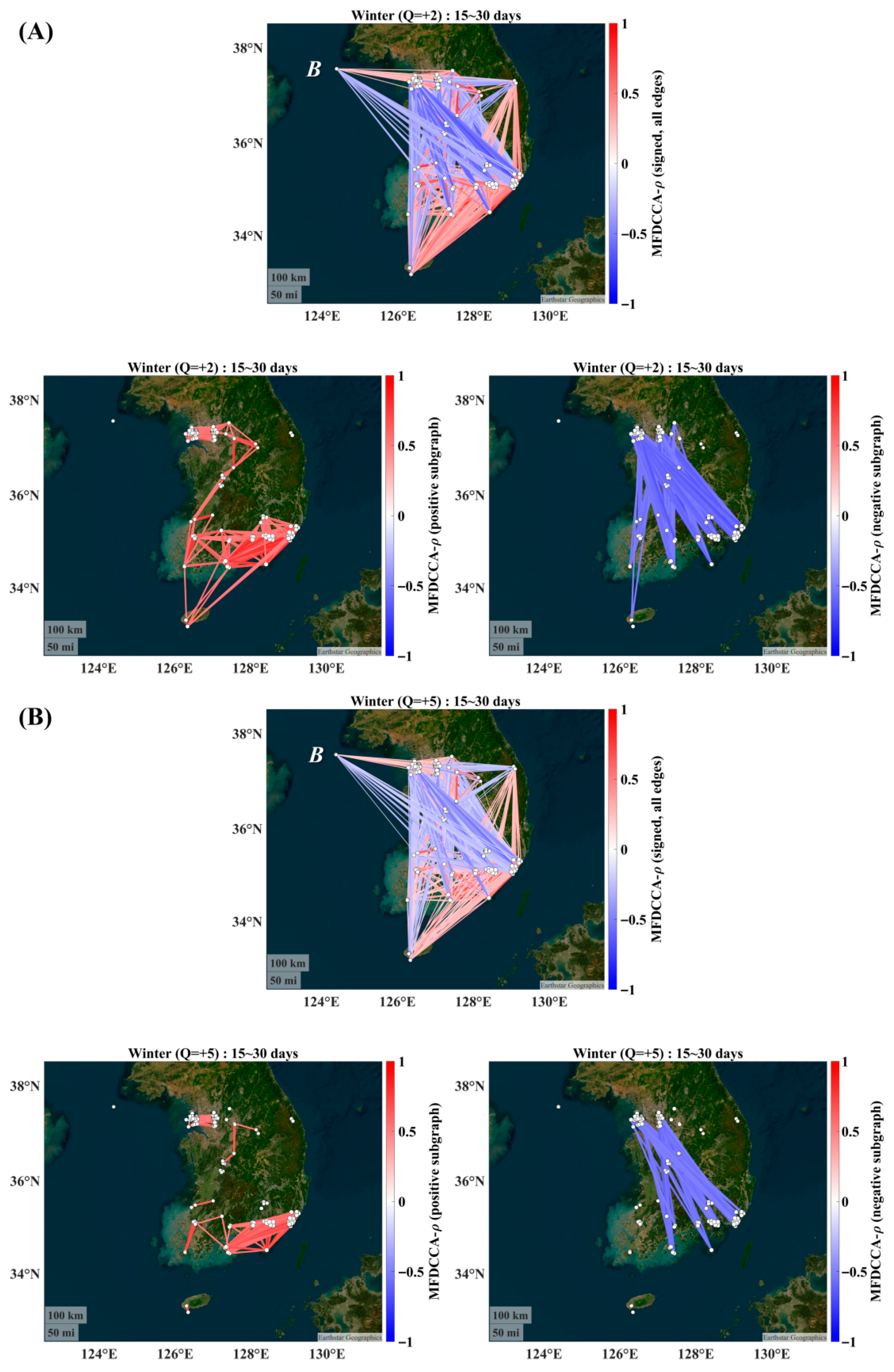
Signed, all-edges view ($\mathit{q}\mathbf{=}\mathbf{+}\mathbf{2} \mathbf{and}\mathbf{+}\mathbf{5}$): Winter exhibits the densest and strongest $q>0$ networks (Figure 7A,B and Figure 8A,B, top), particularly at 15–30 d. Thick, positive ties radiate from the Seoul metropolitan area and west coast, and the B node again integrates strongly with western/southwestern mainland sites. This is precisely when the westerly and northwesterly inflow and stagnant boundary layers combine to synchronize large PM_2.5 anomalies across stations; prior studies show that during winter transboundary contributions from China can account for ~40% (or more) of the Korean PM_2.5, with a maximum impact on the Seoul metropolitan area [30].

Positive vs. negative subgraphs ($\mathit{q}\mathbf{=}\mathbf{+}\mathbf{2} \mathbf{and}\mathbf{+}\mathbf{5}$): The positive subgraph is almost continent-wide across Korean stations, while the negative subgraph picks out a few long northwest–southeast connections (Figure 7A,B and Figure 8A,B, bottom). This pattern again supports regional anti-phase behavior between the capital region and parts of the southeast industrial coast during certain events, superposed upon a generally in-phase, basin-wide signal in winter. Together with the spring results, this is consistent with the seasonal envelope of the transboundary transport along the westerly storm track and the meteorological control of the accumulation/dispersion over Korea [29,30].

3.5. Network Summary and Link to Global Metrics

In this subsection, we present the summary of global network metrics in

Table 1. Global statistics for the positive subgraphs by season and scale band (5–15 days and 15–30 days) for $q=+2 \mathrm{and} q=+5$. Columns report edge density $\delta$, mean $\left|w\right|$, weighted characteristic path length $L_w$, and assortativity $r_s$. Edges are retained only if statistically significant (iAAFT, $\alpha =0.05$; band-wise significant-scale fraction $\ge 0.5$). No additional magnitude threshold is applied in the numbers shown here.

$\mathit{q}$	$\mathbf{Season}$	Scale	$\mathit{\delta }$	$\left|\mathit{w}\right|$	${\mathit{L}}_{\mathit{w}}$	${\mathit{r}}_{\mathit{s}}$
$q=+2$	Spring	5~15 days	0.3508	0.1870	5.4068	0.5597
		15~30 days	0.3318	0.1782	5.2053	0.6073
	Summer	5~15 days	0.3367	0.1946	5.8434	0.6397
		15~30 days	0.3378	0.2065	5.3975	0.6357
	Autumn	5~15 days	0.3419	0.1752	6.2290	0.4954
		15~30 days	0.2994	0.1195	7.7471	0.4647
	Winter	5~15 days	0.3888	0.2129	6.4392	0.5079
		15~30 days	0.3751	0.2008	6.1835	0.5388
$q=+5$	Spring	5~15 days	0.3473	0.1740	6.2661	0.4641
		15~30 days	0.3049	0.1419	6.5345	0.5656
	Summer	5~15 days	0.2941	0.1420	8.3558	0.6011
		15~30 days	0.2980	0.1502	7.4148	0.5180
	Autumn	5~15 days	0.3295	0.1652	5.7067	0.5199
		15~30 days	0.2674	0.1049	7.4217	0.5406
	Winter	5~15 days	0.3534	0.1583	9.0248	0.4781
		15~30 days	0.3051	0.1263	8.4184	0.5484

and

Table 2. Global statistics for the negative subgraphs (same layout as Table 1).

$\mathit{q}$	$\mathbf{Season}$	Scale	$\mathit{\delta }$	$\left|\mathit{w}\right|$	${\mathit{L}}_{\mathit{w}}$	${\mathit{r}}_{\mathit{s}}$
$q=+2$	Spring	5~15 days	0.4172	0.1845	3.5889	0.0696
		15~30 days	0.3927	0.1758	3.4933	0.0549
	Summer	5~15 days	0.4086	0.1939	3.5446	−0.0270
		15~30 days	0.3837	0.2067	3.2482	0.0602
	Autumn	5~15 days	0.4082	0.1736	3.7462	0.0831
		15~30 days	0.3735	0.1653	3.6393	0.0728
	Winter	5~15 days	0.4320	0.2130	3.2202	0.0473
		15~30 days	0.4221	0.2031	3.1733	0.0475
$q=+5$	Spring	5~15 days	0.3646	0.1567	4.2701	0.0940
		15~30 days	0.3441	0.1319	4.4154	0.0432
	Summer	5~15 days	0.3276	0.1241	4.8972	0.0157
		15~30 days	0.3135	0.1354	4.5073	0.0329
	Autumn	5~15 days	0.3322	0.1069	5.2794	0.0372
		15~30 days	0.2823	0.0938	5.2286	0.1028
	Winter	5~15 days	0.3859	0.1483	4.3051	−0.0248
		15~30 days	0.3481	0.1150	4.8347	−0.0033

. These metrics quantify the visual patterns above (note that no threshold was applied to network metric computations for positive/negative subgraphs).

Positive subgraphs. For $q=+2$, the edge density ($\delta$) ranges from 0.299 to 0.389 with an assortativity of 0.465–0.640 and $L_w=5.21–7.75$; the band-averaged $\delta$ is 0.355 (5–15 days) and 0.336 (15–30 days). For $q=+5$, $\delta$ is 0.267–0.353 with an assortativity of 0.464–0.601 and $L_w=5.71–9.02$; the band-averaged $\delta$ reduces to 0.331 (5–15 days) and 0.294 (15–30 days). Thus, positive subnetworks are consistently assortative with moderate densities, and $\delta$ decreases $\mathrm{and} L_w$ increases as $q$ increases from $+2$ to $+5$.

Negative subgraphs. For $q=+2$, $\delta$ is 0.374–0.432, $L_w=3.17–3.75$, and the assortativity is near-neutral ($-0.027$ to $0.083$), with the band-averaged $\delta$ being 0.417 (5–15 days) and 0.393 (15–30 days). For $q=+5$, $\delta$ is 0.282–0.386, $L_w=4.27–5.28$, and the assortativity remains near-neutral with the band-averaged $\delta$ being 0.353 (5–15 days) and 0.322 (15–30 days). Overall, negative subgraphs often show higher $\delta$ than in the short band, yet with a near-zero assortativity and shorter $L_w$ (at $q=+2$), highlighting anti-phase long links rather than clustered like-with-like ties.

These numerical summaries are consistent with the signed maps (Figure 1, Figure 2, Figure 3, Figure 4, Figure 5, Figure 6, Figure 7 and Figure 8): positive edges form assortative regional backbones, whereas negative edges pick out NW-SE anti-phase couplings. The $q$ increase ($+2\to +5$) generally reduces $\delta$ and increases $L_w$, reflecting that a stricter emphasis on large fluctuations yields fewer/longer effective paths after significance testing (and any optional magnitude filtering).

Interpretation. The absence of connectivity for $q<0$ implies that low-amplitude daily fluctuations do not cross-correlate strongly across stations after removing the seasonal cycle and the wide effect (residual analysis; Figure A2). In contrast, large-amplitude events ($q>0$) are coherent and seasonally organized—consistent with episodic accumulation/transport, especially in the winter–spring under westerly flow and high-pressure/low-ventilation conditions over Korea. Prior observational and modeling studies report exactly these seasonal controls, spatial patterns, and substantial transboundary contributions in winter–spring [29,30]; our MFDCCA networks recover those signatures from the data without prescribing the physics.

4. Discussion

4.1. Season-Resolved Connectivity and Meteorological Controls

Our season-resolved MFDCCA-$\rho$ networks reveal a consistent organization of the regional PM_2.5 connectivity over the Korean Peninsula: small-amplitude fluctuations ($q<0$) do not form significant networks, whereas large-amplitude fluctuations ($q>0$) produce dense, scale-specific structures—which are strongest in the winter–spring and at 15–30 days. Positive subgraphs are assortative and delineate regional backbones; negative subgraphs expose a northwest–southeast (NW–SE) anti-phase dipole once the peninsula-wide background (EOF1) is removed. These patterns are consistent with independent observational evidence that cool-season synoptic transport and stagnation enhance spatial coherence while summer convection and wet removal disrupt it [29].

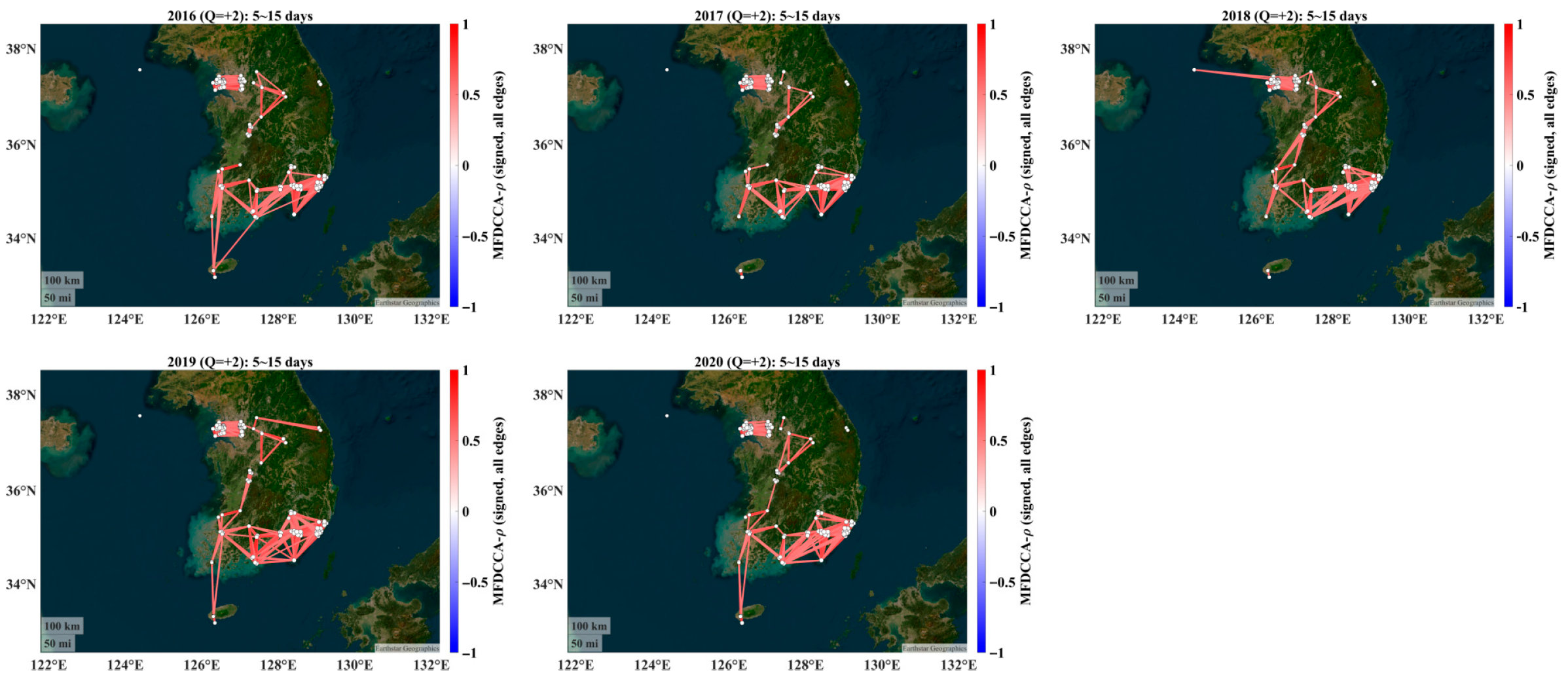
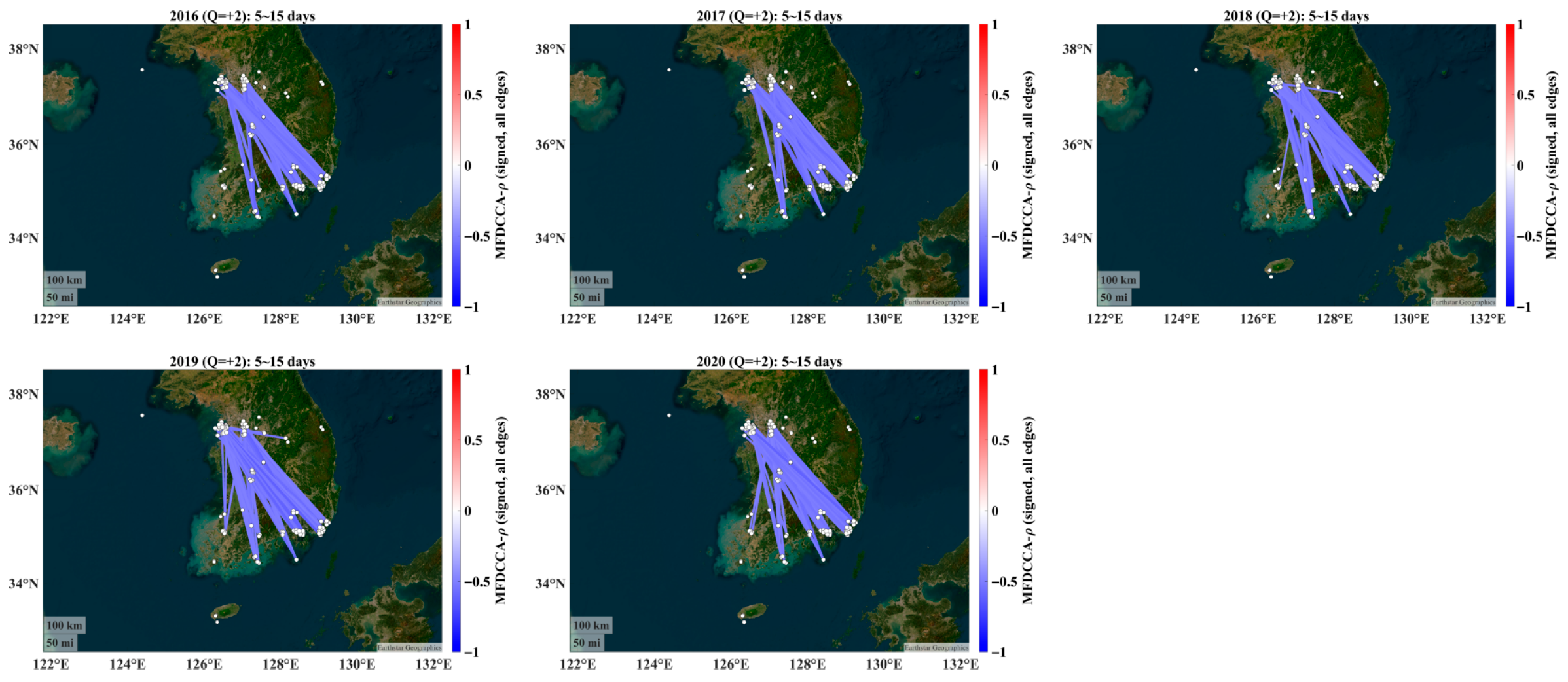
Allabakash et al. [29] (during 2015–2020; same period of our study) reported seasonal PM_2.5 maxima in winter–spring and minima in summer, positive associations with BC/CO/SO₂/SO₄, and negative associations with temperature/precipitation/wind, with a summer-positive coupling with O₃. Crucially, their HYSPLIT backward trajectory analysis [29] for JFM quantified air mass transport percentages from upwind regions, underscoring the cool season transboundary influence. This suite of findings is closely related with our networks: winter–spring positive backbones (through Baengnyeongdo) capture in-phase, transport-enhanced coherence—features that are naturally suppressed in annual aggregation (Figure A3, Figure A5, Figure A7 and Figure A9) but are surfaced here by a season-resolved, fluctuation-level approach.

4.2. Alignment with Annual Features: Year-by-Year Connectivity

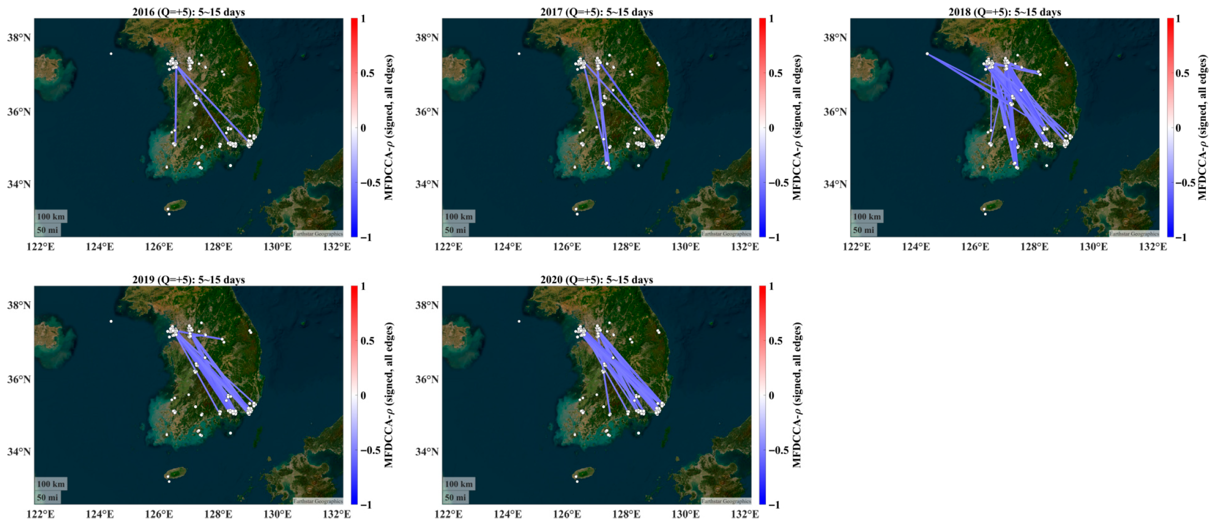
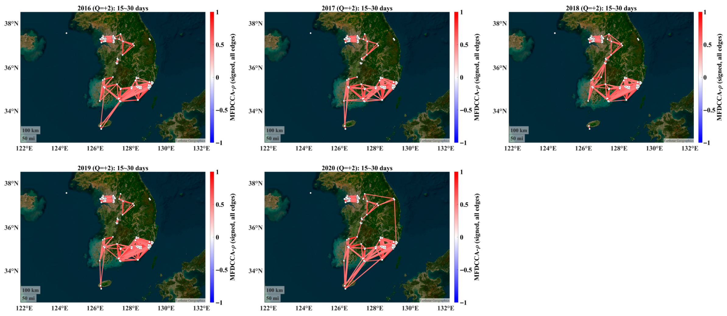
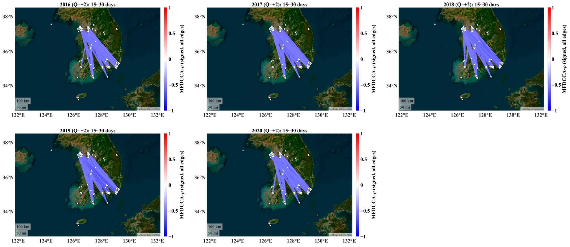
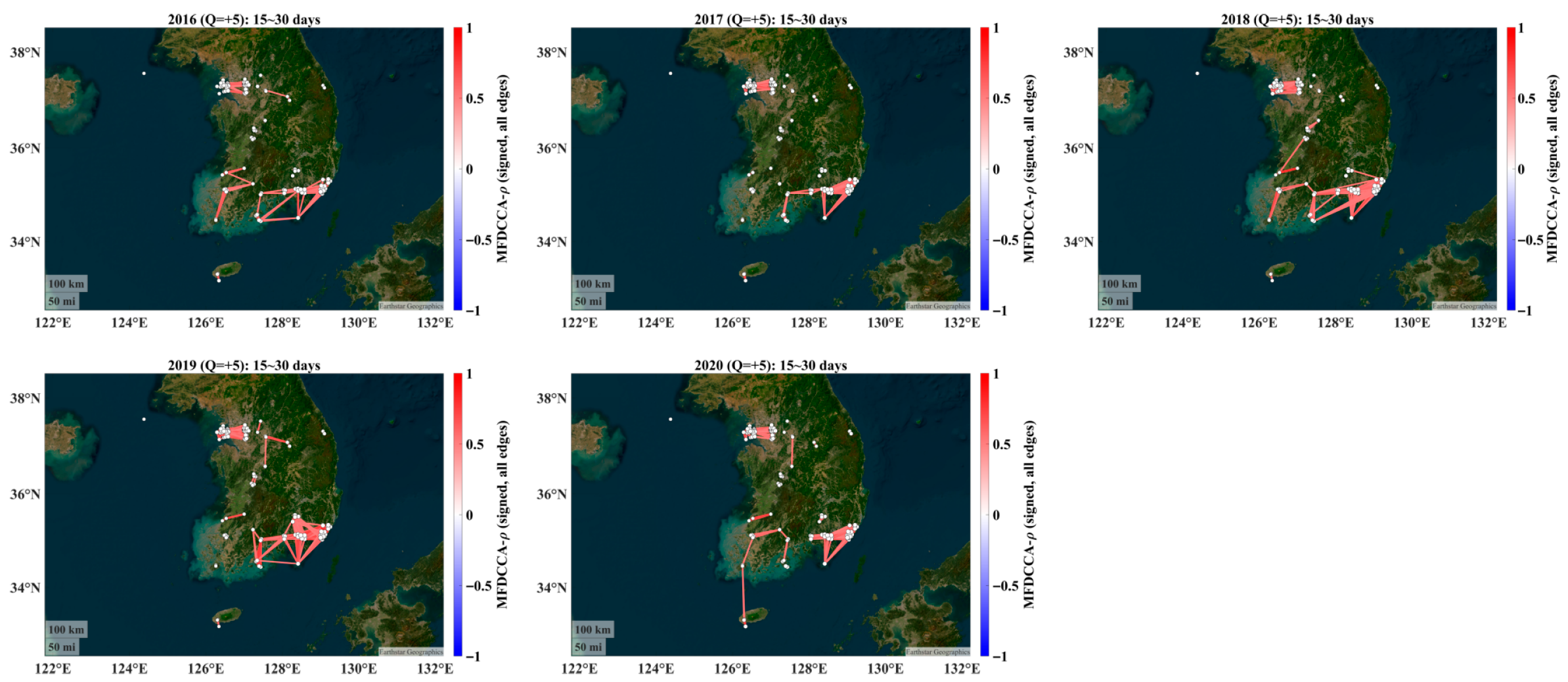
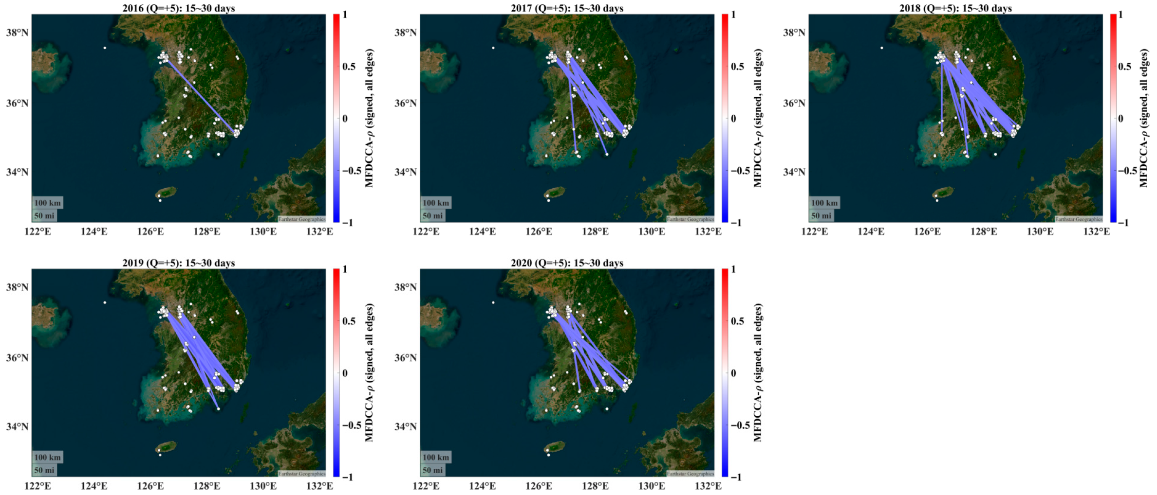
To cross-check the climatology, we compiled year-by-year signed networks for 2016–2020 using the same 5–30-day windows (Figure A3, Figure A4, Figure A5, Figure A6, Figure A7, Figure A8, Figure A9 and Figure A10). Three consistent features emerge:

• The seasonal dominance persists across years. Even when analyzing calendar years, the winter–spring connectivity remains the first-order structure, matching the transport/accumulation regime emphasized by the backward trajectory evidence in the work of Allabakash et al. [29].
• The signed structure is robust. Assortative positive backbones and NW–SE anti-phase negative links recur each year; their edge density and mean |w| vary inter-annually, plausibly reflecting the synoptic frequency, boundary layer depth, and precipitation differences [15,16]. For example, years with more persistent cool-season haze episodes show denser 15–30-day networks, whereas years with weaker synoptic support display attenuated connectivity—qualitatively consistent with annual narratives in Allabakash et al. [29].
• The statistical power is stronger in annual windows. A single year provides fewer boxes at 15–30 days, reducing the surrogate test power versus the season-pooled (cut-and-stitch) design. Thus, the year-wise connectivity is concordant with the seasonal organization but naturally noisier at the largest analyzed scales.

Overall, the year-by-year maps corroborate the seasonal backbone found here and contextualize inter-annual modulation without altering the central conclusion that connectivity is inherently seasonal under the East Asian monsoon.

4.3. Seasonality vs. Annual Features: Comparability and Limitations

The primary objective of this study is to establish a season-resolved climatology of fluctuation-level ($q$-dependent) connectivity. Pooling DJF/MAM/JJA/SON across 2016–2020 (i) preserves a season-specific organization, (ii) avoids seasonal dilution in annual aggregates, and (iii) ensures adequate box counts for MFDCCA-$\rho$ at 5–30 days under missing data constraints. A year-by-year multifractal comparison is a distinct scope (inter-annual evolution) requiring additional controls for meteorology and emissions and, in practice, a broader scale range (e.g., 30–60 days or 45–90 days) to stabilize statistics in single-year segments. For comparability with our seasonal baseline, Appendix A (Figure A3, Figure A4, Figure A5, Figure A6, Figure A7, Figure A8, Figure A9 and Figure A10) retained 5–30 days; a full annual study—optimizing scales and adding meteorological covariates (e.g., trajectory clusters, stagnation indices, and precipitation days)—is therefore reserved for future work. This separation prevents scope drift while providing readers with a reference set of annual connectivity maps alongside the seasonal networks that are the focus here.

4.4. Mechanistic Synthesis and Implications

The joint picture from the season-resolved networks (this study) and backward trajectory/multivariate evidence by Allabakash et al. [29] is that the cool-season westerly inflow, synoptic-scale transport, and stagnation drive episode-scale coherence (densifying positive backbones and clarifying anti-phase links), whereas the summer convection and wet scavenging break connectivity. The Baengnyeongdo (B) node repeatedly acts as a transboundary sentinel during cool seasons—a spatial anchor visible in our signed graphs and physically plausible under the recurrent Yellow Sea inflow.

These insights suggest two immediate uses: (i) episode-scale transboundary diagnostics using network measures (e.g., density, $L_w$, assortativity) in concert with trajectory analysis and (ii) model benchmarking at 5–30-day scales, where a connectivity-based structure complements concentration-based metrics. Extending to annual segmentation, we recommend larger scales and explicit meteorological controls to attribute inter-annual differences in the network topology.

5. Conclusions

This study establishes a season-resolved climatology of the fluctuation-level regional connectivity of PM_2.5 over the Korean Peninsula using sign-preserving MFDCCA-$\rho (q,s$) and surrogate-tested signed networks on EOF1-removed residuals. In brief, small-amplitude fluctuations ($q<0$) do not organize into significant networks, whereas large-amplitude fluctuations ($q>0$) form seasonally and scale-specifically structured networks—which are most pronounced in winter–spring and at 15–30 days. After removing the peninsula-wide background, positive subgraphs are assortative and delineate regional backbones, while negative subgraphs highlight NW-SE anti-phase dipoles; the Baengnyeongdo (B) recurrently acts as a transboundary sentinel in cool seasons [15].

The seasonality and scale preference align with East Asian meteorology: winter–spring westerlies, frequent stagnation, and synoptic-scale transport foster episode-level coherence, whereas summer convection/precipitation disrupts persistence and cross-site coupling [29]. The NW-SE anti-phase links indicate regional phase differences superposed on a basin-wide background that is effectively reduced by the EOF1 removal. These results demonstrate the value of a fluctuation-level lens for revealing the regional PM_2.5 connectivity that would otherwise be masked by a peninsula-wide background.

A fluctuation-level lens ($q$ dependence) plus signed network decomposition separates in-phase (positive) from anti-phase (negative) structures and reveals a seasonal organization that would be blurred by annual aggregation. The surrogate-based decision rule and scale band aggregation provide a rigorous yet interpretable pathway from a multifractal analysis of the regional network topology.

The season-resolved baseline presented here is directly usable for (i) diagnosing transboundary episodes (e.g., through the connectivity of Baengnyeong), (ii) benchmarking chemical transport models at event scales (5–30 days), and (iii) designing monitoring strategies that treat positive and negative subgraphs as complementary signals of regional co-variability.

Since our study focuses on seasonal climatology, future work will extend to (i) inter-annual variability and trend attribution, (ii) multi-pollutant and meteorological covariates, (iii) directionality/lag structures (causal networks), and (iv) stricter multiple-testing control and spatially constrained nulls. Together, these steps will leverage the season-resolved baseline reported here to understand how regional connectivity changes over time.

References

1. Kim, K.-H.; Kabir, E.; Kabir, S. A review on the human health impact of airborne particulate matter. Environ. Int. 2015, 74, 136–143. [Google Scholar] [CrossRef]
2. Srimuruganandam, B.; Nagendra, S. Source characterization of PM10 and PM2.5 mass using a chemical mass balance model at urban roadside. Sci. Total Environ. 2012, 433, 8–19. [Google Scholar] [CrossRef]
3. De-Kok, T.M.C.M.; Driece, H.A.L.; Hogervorst, J.G.F.; Briede, J.J. Toxicological assessment of ambient and traffic—Related particulate matter: A review of recent studies. Mutat. Res. 2006, 613, 103–122. [Google Scholar] [CrossRef] [PubMed]
4. Misra, C.; Geller, M.D.; Shah, P.; Sioutas, C.; Solomon, P.A. Development and evaluation of a continuous coarse (PM10–PM2.5) particle monitor. J. Air Waste Manag. Assoc. 2001, 51, 1309–1317. [Google Scholar] [CrossRef]
5. Johansson, C.; Norman, M.; Gidhagen, L. Spatial & temporal variations of PM10 and particle number concentrations in urban air. Environ. Monit. Assess. 2007, 127, 477–487. [Google Scholar]
6. Cheung, K.; Daher, N.; Kam, W.; Shafer, M.M.; Ning, Z.; Schauer, J.J.; Sioutas, C. Spatial and temporal variation of chemical composition and mass closure of ambient coarse articulate matter (PM10–2.5) in the Los Angeles area. Atmos. Environ. 2011, 45, 2651–2662. [Google Scholar] [CrossRef]
7. Ocak, S.; Turalioglu, F.S. Effect of meteorology on the atmospheric concentrations of traffic-related pollutants in Erzurum, Turkey. J. Int. Environ. Appl. Sci. 2008, 3, 325–335. [Google Scholar]
8. Zhang, H.; Wang, Y.; Hu, J.; Ying, Q.; Hu, X.M. Relationships between meteorological parameters and criteria air pollutants in three megacities in China. Environ. Res. 2015, 140, 242–254. [Google Scholar] [CrossRef]
9. Haddad, K.; Vizakos, N. Air quality pollutants and their relationship with meteorological variables in four suburbs of Greater Sydney, Australia. Air Qual. Atmos. Health 2021, 14, 55–67. [Google Scholar] [CrossRef]
10. Liu, Y.; Zhou, Y.; Lu, J. Exploring the relationship between air pollution and meteorological conditions in China under environmental governance. Sci. Rep. 2020, 10, 1–11. [Google Scholar] [CrossRef]
11. Li, X.; Ma, Y.; Wang, Y.; Liu, N.; Hong, Y. Temporal and spatial analyses of particulate matter (PM10 and PM2.5) and its relationship with meteorological parameters over an urban city in northeast China. Atmos. Res. 2017, 198, 185–193. [Google Scholar] [CrossRef]
12. Caramagna, A.; Famoso, F.; Lanzafame, R.; Monforte, P. Analysis of vertical profile of particulates dispersion in function of the aerodynamic diameter at a congested road in Catania. Energy Procedia 2015, 82, 702–707. [Google Scholar] [CrossRef]
13. Kumar, N.; Park, R.J.; Jeong, J.I.; Woo, J.H.; Kim, Y.; Johnson, J.; Yarwood, G.; Kang, S.; Chun, S.; Knipping, E. Contributions of international sources to PM2. 5 in South Korea. Atmos. Environ. 2021, 261, 118542. [Google Scholar] [CrossRef]
14. Lee, S.; Kim, J.; Choi, M.; Hong, J.; Lim, H.; Eck, T.F.; Holben, B.N.; Ahn, J.Y.; Kim, J.; Koo, J.H. Analysis of long-range transboundary transport (LRTT) effect on Korean aerosol pollution during the KORUS-AQ campaign. Atmos. Environ. 2019, 204, 53–67. [Google Scholar] [CrossRef]
15. Yim, S.H.L.; Gu, Y.; Shapiro, M.A.; Stephens, B. Air quality and acid deposition impacts of local emissions and transboundary air pollution in Japan and South Korea. Atmos. Chem. Phys. 2019, 19, 13309–13323. [Google Scholar] [CrossRef]
16. Choi, J.; Park, R.J.; Lee, H.M.; Lee, S.; Jo, D.S.; Jeong, J.I.; Henze, D.K.; Woo, J.H.; Ban, S.J.; Lee, M.D.; et al. Impacts of local vs. trans-boundary emissions from different sectors on PM2.5 exposure in South Korea during the KORUS-AQ campaign. Atmos. Environ. 2019, 203, 196–205. [Google Scholar] [CrossRef]
17. Lim, G.; Min, S. Correlation Structures of PM2.5 Concentration Series in the Korean Peninsula. Appl. Sci. 2019, 9, 5441. [Google Scholar] [CrossRef]
18. Podobnik, B.; Stanley, H.E. Detrended cross-correlation analysis: A new method for analyzing two nonstationary time series. Phys. Rev. Lett. 2008, 100, 084102. [Google Scholar] [CrossRef] [PubMed]
19. Zhou, W.-X. Multifractal detrended cross-correlation analysis for two nonstationary signals. Phys. Res. E 2008, 77, 066211. [Google Scholar] [CrossRef]
20. Oświecimka, P.; Drożdż, S.; Forczek, M.; Jadach, S.; Kwapień, J. Detrended cross-correlation analysis consistently extended to multifractality. Phys. Res. E 2014, 89, 023305. [Google Scholar] [CrossRef]
21. Schreiber, T.; Schmitz, A. Surrogate time series. Phys. D Nonlinear Phenom. 2000, 142, 346–382. [Google Scholar] [CrossRef]
22. Available online: https://www.airkorea.or.kr/web/pmRelay?itemCode=10007&pMENU_NO=108 (accessed on 1 April 2021).
23. Kwapień, J.; Oświęcimka, P.; Drożdż, S. Detrended fluctuation analysis made flexible to detect range of cross-correlated fluctuations. Phys. Rev. E 2015, 92, 052815. [Google Scholar] [CrossRef]
24. Kantelhardt, J.W.; Zschiegner, S.A.; Bunde, E.K.; Havlin, S.; Bunde, A.; Stanley, H.E. Multifractal detrended fluctuation analysis of nonstationary time series. Phys. A 2002, 316, 87–114. [Google Scholar] [CrossRef]
25. Podobnik, B.; Jiang, Z.-Q.; Zhou, W.-X.; Stanley, H.E. Statistical tests for power-law cross-correlated processes. Phys. Rev. E 2011, 84, 066118. [Google Scholar] [CrossRef]
26. Barrat, A.; Barthélemy, M.; Pastor-Satorras, R.; Vespignani, A. The architecture of complex weighted networks. Proc. Natl. Acad. Sci. USA 2004, 101, 3747–3752. [Google Scholar] [CrossRef]
27. Newman, M.E.J. Assortative Mixing in Networks. Phys. Rev. Lett. 2002, 89, 208701. [Google Scholar] [CrossRef] [PubMed]
28. Newman, M.E.J. Mixing patterns in networks. Phys. Rev. E 2003, 67, 026126. [Google Scholar] [CrossRef] [PubMed]
29. Allabakash, S.; Lim, S.; Chong, K.-S.; Yamada, T.J. Particulate Matter Concentrations over South Korea: Impact of Meteorology and Other Pollutants. Remote Sens. 2022, 14, 4849. [Google Scholar] [CrossRef]
30. Jun, M.-J.; Gu, Y. Effects of transboundary PM2.5 transported from China on the regional PM2.5 concentrations in South Korea: A spatial panel-data analysis. PLoS ONE 2023, 18, e0281988. [Google Scholar] [CrossRef]
Figure 1. Spring connectivity (5–15 days); (A) for q = + 2 ,   (B) for q = +5. Top: Signed, all-edges MFDCCA- ρ network of daily PM2.5 residuals over the Korean Peninsula. Edges are shown only if they are significant against 100 iAAFT surrogates at α = 0.05 and satisfy ρ 0.5 ; color encodes sign (red = positive, blue = negative) and intensity encodes ρ (scale bar at right). Node locations are ground monitoring stations; B marks Baengnyeongdo. Bottom: Signed subgraphs (left: positive; right: negative) extracted from the same network. Basemap: satellite imagery for geographical context.
Fractalfract 09 00737 g001aFractalfract 09 00737 g001b
Figure 2. Spring connectivity (15–30 days); (A) for q = +2, (B) for q = +5. Same layout and criteria as Figure 1 but for the mid band. The network thickens and fills, with strong coast-to-coast positive connectivity and a sparse northwest–southeast negative backbone.
Fractalfract 09 00737 g002
Figure 3. Summer connectivity (5–15 days); (A) for q = +2, (B) for q = +5.Each top panel shows the signed, all-edges network for the given q ; bottom panels show the positive and negative subgraphs. Relative to spring, summer networks are thinner and more fragmented, especially inland, reflecting the weaker cross-site coherence of large fluctuations in the warm season.
Fractalfract 09 00737 g003
Figure 4. Summer connectivity (15–30 days); (A) for q = +2, (B) for q = +5. Same as Figure 3 but for the mid band. Connectivity partially recovers at 15–30 days, with positive edges consolidating along coasts and urban corridors; negative edges remain sparse.
Fractalfract 09 00737 g004
Figure 5. Autumn connectivity (5–15 days); (A) for q = +2, (B) for q = +5. Signed, all-edges maps (top) and the corresponding subgraphs (bottom). The network strengthens relative to summer, with B again integrating strongly into the western backbone; negative ties preferentially bridge northwest southeast.
Fractalfract 09 00737 g005
Figure 6. Autumn connectivity (15–30 days); (A) for q = +2, (B) for q = +5. As in Figure 5 but for the mid band. A nearly peninsula-wide positive network emerges; the negative subgraph remains selective and long-range.
Fractalfract 09 00737 g006
Figure 7. Winter connectivity (5–15 days); (A) for q = +2, (B) for q = +5. The densest short-band networks. Positive edges become ubiquitous, with thick linkages over the capital region and along the western corridor; the negative subgraph preserves a few long northwest–southeast connections.
Fractalfract 09 00737 g007
Figure 8. Winter connectivity (15–30 days); (A) for q = +2, (B) for q = +5. Same as Figure 7 but at 15–30 days. The network is near-percolated with strong positive connectivity throughout; negative links remain sparse and long-range.
Fractalfract 09 00737 g008