Lyapunov-Based Analysis of Partial Practical Stability in Tempered Fractional Calculus

Abstract

This study presents a comprehensive Lyapunov-based framework for analyzing partial practical stability in nonlinear tempered fractional-order systems (TFOS). We develop novel stability concepts including ${\beta }^{*}$-practical uniform generalized Mittag–Leffler stability (${\beta }^{*}$-PUGMLS) and ${\beta }^{*}$-practical uniform exponential stability (${\beta }^{*}$-PUES) with respect to system substates. Through carefully constructed Lyapunov functions, we establish sufficient conditions under which the system’s states converge to a predefined neighborhood of the origin. The theoretical framework provides Mittag–Leffler and exponential stability criteria for tempered fractional-order systems, extending classical stability theory to this important class of systems. Furthermore, we apply these stability results to design stabilizing feedback controllers for a specific class of triangular TFOS, demonstrating the practical utility of our theoretical developments. The efficacy of the proposed stability criteria and control strategy is validated through several illustrative examples, showing that system states converge appropriately under the derived conditions. This work contributes significantly to the stability theory of fractional-order systems and provides practical tools for controlling complex nonlinear systems in the tempered fractional calculus framework.

1. Introduction

Stability theory is a cornerstone of system analysis and control [1,2,3,4,5]. The introduction of the Lyapunov Direct Method (LDM) marked a pivotal advancement, providing a powerful framework for analyzing the stability of nonlinear systems without requiring explicit solutions to their differential equations [6]. Among the types of stability studied is the so-called practical stability, which was examined in [7,8,9,10]. Recent advances in fractional calculus have further expanded the tools available for stability analysis, with significant contributions in various domains including gradient-based optimization algorithms for optimal control problems with general conformable fractional derivatives [11], practical observer design for nonlinear systems [12], finite time stability analysis for Hadamard fractional-order systems [13], and fault-tolerant control strategies for complex systems [14,15]. Fundamental mathematical contributions have also been made through extensions of classical lemmas such as Barbalat’s lemma for generalized conformable fractional integrals [16], alongside comprehensive frameworks for observer design in energy systems [17] and synchronization techniques for mutual coupled fractional-order systems [18]. Additionally, sophisticated approaches for fault estimation in nonlinear one-sided Lipschitz systems [19] and observer-based control methodologies for fractional-order systems [20] have significantly enriched the theoretical foundation for analyzing complex dynamical systems.

In recent years, the utilization of fractional calculus has become increasingly prevalent across various applications, leading to enhanced accuracy in numerous phenomena and models through its application [21,22,23,24,25]. Consequently, a substantial number of researchers have shown considerable interest in conducting advanced investigations into the stability analysis and control of systems involving fractional calculus [26,27,28,29,30]. Notably, the work in [29] established foundational results on the practical stability for a class of fractional-order systems.

The superior modeling ability of tempered fractional derivatives compared to standard fractional operators is the motivation for their study in the literature. Classical fractional derivatives with power-law kernels are able to well describe long-range memory and non-locality; however, they fail to capture exponentially decaying memory as opposed to algebraically decaying memory of a system. The addition of an exponential tempering factor to the fractional derivatives is used to address the weaknesses of an otherwise non-tempered classical model, and it thus provides a model which more accurately represents systems with finite memory or systems with faster-decaying influences than those in the classical power-law regime. Several studies in a variety of fields have realized the benefits of this balanced plan. Often, in the literature of optimization, such as in the Tempered Fractional Gradient Descent algorithm, the convergence behavior is favorable and enhanced stability is demonstrated in the case of stochastic perturbations [31]. In thermal physics, a tempered version of fractional models give a realistic description of the heat dynamics in heterogeneous materials [32,33], and in control theory, they allow the construction of observers with better performance on nonlinear dynamics [34]. The tempering parameter $\tau >0$, therefore, provides not only more modeling flexibility but also an exponential decay that may enhance convergence and enhance stability of dynamical systems—properties that make tempered fractional calculus of particular interest in engineering where memory effects and fast stabilization are of great importance.

This paper makes a key contribution by analyzing the practical stability of TFOS for the general case of $\tau >0$, a significant extension of the existing theory limited to $\tau =0$ in [29]. We demonstrate that a positive tempered parameter induces an exponential decay factor, leading to faster convergence and stronger stability guarantees. Our work also provides a distinct alternative to specialized approaches like the fuzzy-system method of [26]; instead of relying on LMIs, we develop a general Lyapunov-based framework that introduces novel stability concepts (${\beta }^{*}$-PUES, ${\beta }^{*}$-PUGMLS) for a wider class of nonlinear TFOS. Collectively, these developments represent a substantial advancement of the theoretical foundations in this domain. Our contributions are not merely incremental but represent a substantial strengthening of the theoretical framework, as detailed below. The key points of our article can be summarized as follows:

• Stability Results: We establish results on practical Mittag–Leffler stability and practical exponential stability for TFOS.
• Controller Design: A feedback controller is proposed for a class of TFOS to enhance system performance.
• Conceptual Advancement: Unlike [27], which focuses on power systems and uses SOS optimization for polynomial controllers, our work develops a Lyapunov-based framework for partial practical stability in general nonlinear TFOS and introduces two new stability concepts (${\beta }^{*}$-PUGMLS and ${\beta }^{*}$-PUES). Furthermore, we address triangular systems and provide constructive controller design without relying on SOS tools.
• Numerical Validation: Several numerical examples are provided to demonstrate the effectiveness of the proposed results.

We provide a side-by-side comparison with [27,29] in Table 1 to clarify how our contribution differs from prior studies.

Table 1. Comparison between [27,29], and the present work.

Aspect	Ben Makhlouf (2022) [29]	Gassara et al. (2023) [27]	This Paper
Fractional operator	Caputo ($\tau =0$)	Tempered Caputo ($\tau >0$)	Tempered Caputo ($\tau >0$)
Problem setting	Partial practical stability of nonlinear FOS	Practical stabilization of power systems	Partial practical stability of general nonlinear TFOS
Main notions	Partial practical stability	Practical Mittag–Leffler stability (PMLS)	${\beta }^{*}$-PUGMLS and ${\beta }^{*}$-PUES (new concepts)
Methodology	Lyapunov inequalities	SOS optimization for polynomial controller	Lyapunov-based framework with new comparison bounds for tempered kernels
Convergence rate	Mittag–Leffler decay	Mittag–Leffler decay with tempered factor	Exponential × ML decay (faster due to $e^{-\tau t}$)
Scope of systems	General Caputo FOS + triangular class	Power systems only	General TFOS + triangular class with feedback design
Controller design	Yes (triangular systems)	Polynomial controller via SOS	Constructive state feedback for triangular TFOS
Partial (substate) results	Yes	Not considered	Yes stability with respect to $x^1$ substate
Numerical evidence	Examples without $\tau$	Power system simulations	Full-state trajectories, robustness vs. $\tau$, semi-log plots
Relation to the tempered literature	Not applicable (Caputo only)	First SOS-based approach for tempered PS	First Lyapunov-based framework for partial practical stability in TFOS

Unlike [27,29], our work introduces new stability notions, addresses partial practical stability in the tempered case, and provides constructive controller design for triangular TFOS. The tempered parameter enables provably faster convergence, validated analytically and numerically.

This article is structured as follows: Section 2 contains some preliminary findings. We examine the practical Mittag–Leffler exponential stability for TFOS in Section 3. In Section 4, a feedback controller for a class of TFOS is developed.

2. Preliminaries

This section covers the basics of tempered fractional calculus.

Definition 1

([35]). Let $\iota >0,\tau \ge 0$, and $f\in C\left([c_1,c_2],\mathbb{R}\right)$. The tempered fractional integral of order ι of f is given by

$$\begin{array}{cc}\hfill I_{c_1^{+}}^{\iota ,\tau }f\left(\varkappa \right)& ={\displaystyle \frac{1}{\mathsf{\Gamma }\left(\iota \right)}}{\int }_{c_1}^{\varkappa }{\left(\varkappa -l\right)}^{\iota -1}exp(-\tau \left(\varkappa -l\right))f\left(l\right)dl.\hfill \end{array}$$

Definition 2

([35]). Let $0<\iota <1$ and $\tau \ge 0$. The Caputo tempered fractional derivative of order ι for $f\in AC[c_1,c_2]$ is given by

$${}^{C}D_{c_1^{+}}^{\iota ,\tau }f\left(\varkappa \right)={\displaystyle \frac{exp(-\tau \varkappa )}{\mathsf{\Gamma }(1-\iota )}}{\int }_{c_1}^{\varkappa }{\left(\varkappa -w\right)}^{-\iota }{\displaystyle \frac{d}{dw}}\left(exp(\tau w)f(w)\right)dw.$$

(1)

Definition 3

([36]). The Mittag–Leffler function is defined by

$${\displaystyle E_{l_1,l_2}\left(z\right)=\sum _{\kappa =0}^{+\infty }\frac{z^{\kappa }}{\mathsf{\Gamma }(\kappa l_1+l_2)},}$$

where $l_1>0$, $l_2>0$, $z\in \mathbb{C}$.

If $l_2=1$, we note $E_{l_1}\left(z\right)=E_{l_1,1}\left(z\right)$.

Lemma 1

([37]). For $l_1\in (0,2]$, we have

$$E_{l_1,l_2}\left(x^{l_1}\right)\sim x^{1-l_2}{\displaystyle \frac{e^x}{l_1}},x⟼\infty .$$

Lemma 2

([38]). For $\iota >0$, we have

$${\displaystyle \frac{1}{\mathsf{\Gamma }\left(\iota \right)}}{\int }_0^{\varkappa }{(\varkappa -w)}^{\iota -1}{e}^{rw}dw={\varkappa }^{\iota }{E}_{1,\iota +1}\left(r\varkappa \right).$$

Lemma 3

([35]). Let $y:[c_1,c_2]⟶{\mathbb{R}}^n$ be an absolutely continuous function and $P\in {\mathbb{R}}^{n\times n}$ with $P=P^T$, then

$${}^{C}D_{c_1^{+}}^{\iota ,\tau }{y}^{T}Py\left(\varkappa \right)\le 2y{\left(\varkappa \right)}^T{P}^C{D}_{a^{+}}^{\iota ,\tau }y\left(\varkappa \right).$$

(2)

Lemma 4

([35]). The solution of the following system

$${}^{C}D_{{{\varkappa }_0}^{+}}^{\iota ,\tau }v\left(\varkappa \right)=c_{1}v+c_2\left(\varkappa \right),\varkappa \ge {\varkappa }_0$$

(3)

with $v\in {\mathbb{R}}^n$, is given by

$$\begin{array}{ccc}\hfill v\left(\varkappa \right)& =& exp(-\tau (\varkappa -{\varkappa }_0))E_{\iota }\left(c_1{(\varkappa -{\varkappa }_0)}^{\iota }\right)u\left({\varkappa }_0\right)\hfill \\ & +& {\int }_{{\varkappa }_0}^{\varkappa }{(\varkappa -s)}^{\iota -1}{E}_{\iota ,\iota }(c_1{(\varkappa -s)}^{\iota })exp(-\tau (\varkappa -s))c_2\left(s\right)ds.\hfill \end{array}$$

(4)

Lemma 5

([39]). The function $s⟼E_r(-s)$ is nonincreasing for all $0<r<1$.

Definition 4

([4]). A function $f\in C\left({\mathbb{R}}_{+},{\mathbb{R}}_{+}\right)$ is said to be in the class $\mathcal{K}$ if it is increasing and $f\left(0\right)=0$. In addition, if ${\displaystyle \underset{r⟶+\infty }{lim}f\left(r\right)=+\infty }$, then it is in the class ${\mathcal{K}}_{\infty }$.

Lemma 6

([4]). For $f\in \mathcal{K}$, we have for all $l_1,l_2\ge 0$

$$f(l_1+l_2)\le f\left(2l_1\right)+f\left(2l_2\right).$$

Lemma 7

([40]). If $d_1,d_2\ge 0$, and $w\ge 1$, then ${(d_1+d_2)}^w\le 2^{w-1}(d_1^w+d_2^w)$ and ${(d_1+d_2)}^{{\displaystyle \frac{1}{w}}}\le (d_1^{{\displaystyle \frac{1}{w}}}+d_2^{{\displaystyle \frac{1}{w}}})$.

3. Main Results

Consider the following TFOS:

$$\begin{array}{ccc}\hfill {}^{C}D_{{\omega }_0^{+}}^{\iota ,\tau }\varpi \left(\varkappa \right)& =& G(\varkappa ,\varpi ,\beta ),\varkappa \ge {\omega }_0,\hfill \\ \hfill \varpi \left({\omega }_0\right)={\varpi }_0& =& ({\varpi }_0^1,{\varpi }_0^2),\hfill \\ \hfill \varpi \in {\mathbb{R}}^n,\varpi =({\varpi }^1,{\varpi }^2)& ,& {\varpi }^1\in {\mathbb{R}}^{n_1},{\varpi }^2\in {\mathbb{R}}^{n_2},n_1>0,n_2>0,n_1+n_2=n,\hfill \end{array}$$

(5)

where $0<\iota <1$, ${\omega }_0\ge 0$, $\beta >0$, and $G(.,.,\beta ):{\mathbb{R}}_{+}\times {\mathbb{R}}^n⟶{\mathbb{R}}^n$ is a smooth function such that the existence and uniqueness of solution ${\varpi }_{\beta }(\varkappa ;{\omega }_0,{\varpi }_0)\in C[{\omega }_0,+\infty )\cap C^1({\omega }_0,+\infty )$ is ensured (some results about the existence, uniqueness, and regularity of the solutions are given in [41,42]).

Definition 5.

The TFOS (5) is said to be

(i) 

${\beta }^{*}$-practically uniformly exponentially stable with respect to ${\varpi }^1$ (${\beta }^{*}$-PUES-${\varpi }^1$), if for every $0<\beta \le {\beta }^{*}$, there is $d_1\left(\beta \right)>0$, $d_2\left(\beta \right)>0$, and $d_3\left(\beta \right)>0$ such that for every $\varkappa \ge {\omega }_0\ge 0$

$$\parallel {\varpi }_{\beta }^1(\varkappa ;{\omega }_0,{\varpi }_0)\parallel \le d_1\left(\beta \right)\parallel {\varpi }_0\parallel e^{-d_2\left(\beta \right)(\varkappa -{\omega }_0)}+d_3\left(\beta \right)$$

(6)

with $d_3\left(\beta \right)⟶0$ as $\beta ⟶0^{+}$ and there is $H,b_1,b_2>0$ with $0<d_1\left(\beta \right)\le H$, $b_1\le d_2\left(\beta \right)\le b_2$ for all $\beta \in (0,{\beta }^{*}]$.

(ii) 

${\beta }^{*}$-practically uniformly generalized Mittag–Leffler stable with respect to ${\varpi }^1$ (${\beta }^{*}$-PUGMLS-${\varpi }^1$), if for every $0<\beta \le {\beta }^{*}$, there is $d_1\left(\beta \right)>0$, $d_2\left(\beta \right)>0$, $d_3\left(\beta \right)>0$, and $d_4\left(\beta \right)>0$ such that for every $\varkappa \ge {\omega }_0\ge 0$

$$\parallel {\varpi }_{\beta }^1(\varkappa ;{\omega }_0,{\varpi }_0)\parallel \le d_1\left(\beta \right)\parallel {\varpi }_0\parallel e^{-d_2\left(\beta \right)(\varkappa -{\omega }_0)}{\left[E_{\upsilon }\left(-d_3\left(\beta \right){\left(\iota \left(\varkappa \right)-\iota \left({\omega }_0\right)\right)}^{\upsilon }\right)\right]}^q+d_4\left(\beta \right)$$

(7)

with $q>0$, $d_4\left(\beta \right)⟶0$ as $\beta ⟶0^{+}$ and there is $H,c_1,c_2,b_1,b_2>0$ with $0<d_1\left(\beta \right)\le H$, $c_1<d_2\left(\beta \right)<c_2$, $b_1\le d_3\left(\beta \right)\le b_2$ for all $\beta \in (0,{\beta }^{*}]$.

Remark 1.

Note that ${\beta }^{*}$-practical uniform generalized Mittag–Leffler stability guarantees faster convergence of solutions than ${\beta }^{*}$-practical uniform exponential stability.

Theorem 1.

Let $\kappa \ge 1$ and ${\beta }^{*}>0$. Suppose that for every $0<\beta \le {\beta }^{*}$, there is a $C^1$ function $V_{\beta }:{\mathbb{R}}_{+}\times {\mathbb{R}}^n⟶\mathbb{R}$, a continuous function $\mu :{\mathbb{R}}_{+}⟶{\mathbb{R}}_{+}$ and $a_1\left(\beta \right)>0$, $a_2\left(\beta \right)>0$, $a_3\left(\beta \right)>0$, $r_1\left(\beta \right)>0,$$r_2\left(\beta \right)>0$ such that

1. 

$$a_1\left(\beta \right)\parallel {\varpi }^1{\parallel }^{\kappa }\le V_{\beta }(\varkappa ,\varpi )\le a_2\left(\beta \right){\parallel \varpi \parallel }^{\kappa }+r_1\left(\beta \right),\forall \varkappa \ge 0,\varpi \in {\mathbb{R}}^n.$$

(8)

2. 

$${}^{C}D_{{\omega }_0^{+}}^{\iota ,\tau }{V}_{\beta }(\varkappa ,{\varpi }_{\beta }(\varkappa ;{\omega }_0,{\varpi }_0))\le -a_3\left(\beta \right){\parallel {\varpi }_{\beta }^1(\varkappa ;{\omega }_0,{\varpi }_0)\parallel }^{\kappa }+\mu \left(\varkappa \right)r_2\left(\beta \right),\forall \varkappa \ge {\omega }_0.$$

(9)

with

• $\forall \beta \in (0,{\beta }^{*}]$, ${\displaystyle \frac{a_3\left(\beta \right)}{a_2\left(\beta \right)}}\ge \lambda$ and $0<{\displaystyle \frac{a_2\left(\beta \right)}{a_1\left(\beta \right)}}\le K$, with λ, $K>0$.
• The function ${\displaystyle \varkappa \mapsto {\int }_0^{\varkappa }{(\varkappa -l)}^{\iota -1}exp\left(-\tau (\varkappa -l)\right)E_{\iota ,\iota }\left(-\lambda {(\varkappa -l)}^{\iota }\right)\mu \left(l\right)dl}$ is bounded.
• $c\left(\beta \right)⟶0$ as $\beta ⟶0^{+}$ where

  $$c\left(\beta \right)=r_1\left(\beta \right){\displaystyle \frac{(a_2\left(\beta \right)+C{a}_3\left(\beta \right))}{a_1\left(\beta \right)a_2\left(\beta \right)}}+r_2\left(\beta \right){\displaystyle \frac{C}{a_1\left(\beta \right)}},$$

  with $C=C_1+C_2$, where

  $${\displaystyle C_1=\underset{s\ge 0}{sup}\left(s^{\iota }{E}_{\iota ,\iota +1}\left(-\lambda s^{\iota }\right)\right)}$$

  and

  $${\displaystyle C_2=\underset{\varkappa \ge 0}{sup}{\int }_0^{\varkappa }{(\varkappa -l)}^{\iota -1}exp\left(-\tau (\varkappa -l)\right)E_{\iota ,\iota }\left(-\lambda {(\varkappa -l)}^{\iota }\right)\mu \left(l\right)dl.}$$

Then, the system (5) is ${\beta }^{*}$-PUGMLS-${\varpi }^1$.

Proof. 

It follows from (8) and (9) that

$$\begin{array}{cc}\hfill {}^{C}D_{{\omega }_0^{+}}^{\iota ,\tau }{V}_{\beta }(\varkappa ,{\varpi }_{\beta }(\varkappa ;{\omega }_0,{\varpi }_0))& \le -{\displaystyle \frac{a_3\left(\epsilon \right)}{a_2\left(\epsilon \right)}}{V}_{\beta }(\varkappa ,{\varpi }_{\beta }(\varkappa ;{\omega }_0,{\varpi }_0))+\rho \left(\varkappa \right)l\left(\beta \right)\hfill \\ \hfill & \le -\lambda V_{\beta }(\varkappa ,{\varpi }_{\beta }(\varkappa ;{\omega }_0,{\varpi }_0))+\rho \left(\varkappa \right)l\left(\beta \right),\forall \varkappa \ge {\omega }_0,\hfill \end{array}$$

(10)

where $\rho \left(\varkappa \right)=\left(1+\mu \left(\varkappa \right)\right)$ and $l\left(\beta \right)=r_2\left(\beta \right)+{\displaystyle \frac{r_1\left(\beta \right)a_3\left(\beta \right)}{a_2\left(\beta \right)}}$.

Let

$$\begin{array}{c}\hfill h\left(\varkappa \right){=}^C{D}_{{\omega }_0^{+}}^{\iota ,\tau }{V}_{\beta }(\varkappa ,{\varpi }_{\beta }(\varkappa ;{\omega }_0,{\varpi }_0))+\lambda V_{\beta }(\varkappa ,{\varpi }_{\beta }(\varkappa ;{\omega }_0,{\varpi }_0)).\end{array}$$

(11)

Using Lemma 4, we get

$$\begin{array}{ccc}\hfill V_{\beta }(\varkappa ,{\varpi }_{\beta }(\varkappa ;{\omega }_0,{\varpi }_0))& =& exp\left(-\tau (\varkappa -{\varkappa }_0)\right)E_{\iota }\left(-\lambda {(\varkappa -{\varkappa }_0)}^{\iota }\right)V_{\beta }({\omega }_0,{\varpi }_0)\hfill \\ & +& {\int }_{{\varkappa }_0}^{\varkappa }{(\varkappa -l)}^{\iota -1}{E}_{\iota ,\iota }\left(-\lambda {(\varkappa -l)}^{\iota }\right)exp\left(-\tau (\varkappa -l)\right)h\left(l\right)dl.\hfill \end{array}$$

(12)

Therefore,

$$\begin{array}{ccc}\hfill V_{\beta }(\varkappa ,{\varpi }_{\beta }(\varkappa ;{\omega }_0,{\varpi }_0))& \le & exp\left(-\tau (\varkappa -{\varkappa }_0)\right)E_{\iota }\left(-\lambda {(\varkappa -{\varkappa }_0)}^{\iota }\right)V_{\beta }({\omega }_0,{\varpi }_0)\hfill \\ & +& {\int }_{{\varkappa }_0}^{\varkappa }{(\varkappa -s)}^{\iota -1}{E}_{\iota ,\iota }\left(-\lambda {(\varkappa -s)}^{\iota }\right)exp\left(-\tau (\varkappa -s)\right)\rho \left(s\right)l\left(\beta \right)ds.\hfill \end{array}$$

(13)

Then,

$$\begin{array}{c}\hfill V_{\beta }(\varkappa ,{\varpi }_{\beta }(\varkappa ;{\omega }_0,{\varpi }_0))\le exp\left(-\tau (\varkappa -{\varkappa }_0)\right)E_{\iota }\left(-\lambda {(\varkappa -{\varkappa }_0)}^{\iota }\right)V_{\beta }({\omega }_0,{\varpi }_0)+Cl\left(\beta \right),\forall \varkappa \ge {\omega }_0.\end{array}$$

(14)

It follows from (8) that

$$\parallel {\varpi }_{\beta }^1(\varkappa ;{\omega }_0,{\varpi }_0){\parallel }^{\kappa }\le {\displaystyle \frac{1}{a_1\left(\beta \right)}}exp\left(-\tau (\varkappa -{\varkappa }_0)\right)E_{\iota }\left(-\lambda {(\varkappa -{\varkappa }_0)}^{\iota }\right)\left(a_2\left(\beta \right){\parallel {\varpi }_0\parallel }^{\kappa }+r_1\left(\beta \right)\right)+{\displaystyle \frac{Cl\left(\beta \right)}{a_1\left(\beta \right)}}$$

(15)

Using Lemma 5, we get

$$exp\left(-\tau (\varkappa -{\varkappa }_0)\right)E_{\iota }\left(-\lambda {(\varkappa -{\varkappa }_0)}^{\iota }\right)\le 1.$$

Therefore,

$$\parallel {\varpi }_{\beta }^1(\varkappa ;{\omega }_0,{\varpi }_0){\parallel }^{\kappa }\le {\displaystyle \frac{a_2\left(\beta \right)}{a_1\left(\beta \right)}}exp\left(-\tau (\varkappa -{\varkappa }_0)\right)E_{\iota }\left(-\lambda {(\varkappa -{\varkappa }_0)}^{\iota }\right){\parallel {\varpi }_0\parallel }^{\kappa }+c\left(\beta \right),\varkappa \ge {\omega }_0.$$

(16)

Using Lemma 7, we get

$$\parallel {\varpi }_{\beta }^1(\varkappa ;{\omega }_0,{\varpi }_0)\parallel \le {\left[{\displaystyle \frac{a_2\left(\beta \right)}{a_1\left(\beta \right)}}exp\left(-\tau (\varkappa -{\varkappa }_0)\right)E_{\iota }\left(-\lambda {(\varkappa -{\varkappa }_0)}^{\iota }\right){\parallel {\varpi }_0\parallel }^{\kappa }\right]}^{{\displaystyle \frac{1}{\kappa }}}+r\left(\beta \right),\varkappa \ge {\omega }_0,$$

(17)

Hence,

$$\parallel {\varpi }_{\beta }^1(\varkappa ;{\omega }_0,{\varpi }_0)\parallel \le {\left({\displaystyle \frac{a_2\left(\beta \right)}{a_1\left(\beta \right)}}\right)}^{{\displaystyle \frac{1}{\kappa }}}\parallel {\varpi }_0\parallel exp(-{\displaystyle \frac{\tau }{\kappa }}(\varkappa -{\varkappa }_0)){\left[E_{\iota }\left(-\lambda {(\varkappa -{\varkappa }_0)}^{\iota }\right)\right]}^{{\displaystyle \frac{1}{\kappa }}}+r\left(\beta \right),\varkappa \ge {\omega }_0,$$

(18)

with $r\left(\beta \right)=c{\left(\beta \right)}^{{\displaystyle \frac{1}{p}}}$. Thus, the system (5) is ${\beta }^{*}$-PUGMLS-${\varpi }^1$. □

Remark 2.

While the authors of [29] established the practical stability of the system (5) for $\tau =0$, we show that for $\tau >0$, the convergence of solutions is significantly faster, a result facilitated by the exponential function.

Example 1.

Let the following TFOS

$$\begin{array}{cc}{}^{C}D_{{\omega }_0^{+}}^{\iota ,\tau }{\varpi }_1\hfill & =-2{\varpi }_1+{\varpi }_2+\beta cos\left({\varpi }_1\right),\hfill \\ {}^{C}D_{{\omega }_0^{+}}^{\iota ,\tau }{\varpi }_2\hfill & =-{\varpi }_1-{\varpi }_2+\beta sin\left({\varpi }_2\right)+{\displaystyle \frac{{\beta }^4{\varpi }_1}{{\varpi }_2^2+{\varpi }_1^2+1}},\hfill \\ {}^{C}D_{{\omega }_0^{+}}^{\iota ,\tau }{\varpi }_3\hfill & =2{\varpi }_3,\hfill \end{array}$$

(19)

with $\varpi =\left({\varpi }_1,{\varpi }_2,{\varpi }_3\right)\in {\mathbb{R}}^3$.

For ${\displaystyle \vartheta (\varkappa ,\varpi )=\frac{{\varpi }_1^2+{\varpi }_2^2}{2}}$, we get

$$\begin{array}{ccc}\hfill {}^{C}D_{{\omega }_0^{+}}^{\iota ,\tau }\vartheta (\varkappa ,\varpi (\varkappa ;{\omega }_0,{\varpi }_0))& \le & {\varpi }_1{(\varkappa ;{\omega }_0,{\varpi }_0)}^C{D}_{{\omega }_0^{+}}^{\iota ,\tau }{\varpi }_1(\varkappa ;{\omega }_0,{\varpi }_0)+{\varpi }_2{(\varkappa ;{\omega }_0,{\varpi }_0)}^C{D}_{{\omega }_0^{+}}^{\iota ,\tau }{\varpi }_2(\varkappa ;{\omega }_0,{\varpi }_0)\hfill \\ & \le & -(2-\beta ){\varpi }_1^2-(1-\beta ){\varpi }_2^2+{\beta }^2.\hfill \end{array}$$

(20)

Thus, by using the previous theorem, we get the ${\beta }^{*}$-PUGMLS-${\varpi }^1$ for TFOS (19).

Interpretation: Figure 1 demonstrates the ${\beta }^{*}$-PUGMLS property of the system described in Example 1. The substate $({\varpi }_1,{\varpi }_2)$ converges to a neighborhood of the origin with a radius of less than 0.01, confirming the theoretical prediction. The convergence follows a Mittag–Leffler pattern as expected for tempered fractional systems.

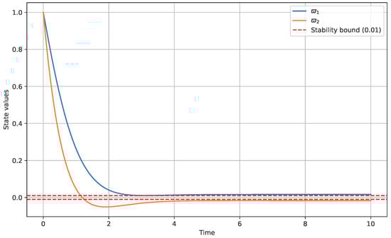
Figure 1. State trajectories for Example 1 with $\iota =0.7$, $\tau =0.5$, and $\beta =0.05$. The substate $({\varpi }_1,{\varpi }_2)$ converges to the ball of radius 0.01 (dashed line).

Theorem 2.

Let $\kappa \ge 1$ and ${\beta }^{*}>0$. Suppose that for every $0<\beta \le {\beta }^{*}$, there is a $C^1$ function $V_{\beta }:{\mathbb{R}}_{+}\times {\mathbb{R}}^n⟶\mathbb{R}$, a continuous function $\mu :{\mathbb{R}}_{+}⟶{\mathbb{R}}_{+}$, $a_1\left(\beta \right)>0$, $a_2\left(\beta \right)>0$, $r_1\left(\beta \right)>0$, $r_2\left(\beta \right)>0$, and $a_3\left(\beta \right)\ge 0$, such that

1. 

$$a_1\left(\beta \right)\parallel {\varpi }^1{\parallel }^{\kappa }\le V_{\beta }(\varkappa ,\varpi )\le a_2\left(\beta \right){\parallel \varpi \parallel }^{\kappa }+r_1\left(\beta \right),\forall \varkappa \ge 0,\varpi \in {\mathbb{R}}^n.$$

(21)

2. 

$${}^{C}D_{{\omega }_0^{+}}^{\iota ,\tau }{V}_{\beta }(\varkappa ,{\varpi }_{\beta }(\varkappa ;{\omega }_0,{\varpi }_0))\le a_3\left(\beta \right){\parallel {\varpi }_{\theta }^1(\varkappa ;{\omega }_0,{\varpi }_0)\parallel }^{\kappa }+\mu \left(\varkappa \right)r_2\left(\beta \right),\forall \varkappa \ge {\omega }_0.$$

(22)

with

• $a_3\left(\beta \right)\le a_1\left(\beta \right)\tilde{a}$ for all $0<\beta \le {\beta }^{*}$ for some $\tilde{a}\in [0,{\tau }^{\iota })$.
• $\forall \beta \in (0,{\beta }^{*}]$, $0<{\displaystyle \frac{a_2\left(\beta \right)}{a_1\left(\beta \right)}}\le K$, with $K>0$.
• The function ${\displaystyle \varkappa \mapsto {\int }_0^{\varkappa }{(\varkappa -s)}^{\iota -1}{E}_{\iota ,\iota }\left(\tilde{a}{(\varkappa -s)}^{\iota }\right)exp\left(-\tau (\varkappa -s)\right)\mu \left(s\right)ds}$ is bounded.
• ${\displaystyle \frac{r_1\left(\beta \right)}{a_1\left(\beta \right)}}⟶0$ and ${\displaystyle \frac{r_2\left(\beta \right)}{a_1\left(\beta \right)}}⟶0$ as $\beta ⟶0^{+}$.

Then, the system (5) is ${\beta }^{*}$-PUES-${\varpi }^1$.

Proof. 

It follows from (21) and (22) that

$$\begin{array}{cc}\hfill {}^{C}D_{{\omega }_0^{+}}^{\iota ,\tau }{V}_{\beta }(\varkappa ,{\varpi }_{\beta }(\varkappa ;{\omega }_0,{\varpi }_0))& \le {\displaystyle \frac{a_3\left(\epsilon \right)}{a_1\left(\epsilon \right)}}{V}_{\beta }(\varkappa ,{\varpi }_{\beta }(\varkappa ;{\omega }_0,{\varpi }_0))+\mu \left(\varkappa \right)r_2\left(\beta \right),\forall \varkappa \ge {\omega }_0.\hfill \end{array}$$

(23)

Let

$$\begin{array}{c}\hfill h\left(\varkappa \right){=}^C{D}_{{\omega }_0^{+}}^{\iota ,\tau }{V}_{\beta }(\varkappa ,{\varpi }_{\beta }(\varkappa ;{\omega }_0,{\varpi }_0))-{\displaystyle \frac{a_3\left(\epsilon \right)}{a_1\left(\epsilon \right)}}{V}_{\beta }(\varkappa ,{\varpi }_{\beta }(\varkappa ;{\omega }_0,{\varpi }_0)).\end{array}$$

(24)

Using Lemma 4, we get

$$\begin{array}{ccc}\hfill V_{\beta }(\varkappa ,{\varpi }_{\beta }(\varkappa ;{\omega }_0,{\varpi }_0))& =& exp\left(-\tau (\varkappa -{\varkappa }_0)\right)E_{\iota }\left({\displaystyle \frac{a_3\left(\epsilon \right)}{a_1\left(\epsilon \right)}}{(\varkappa -{\varkappa }_0)}^{\iota }\right)V_{\beta }({\omega }_0,{\varpi }_0)\hfill \\ & +& {\int }_{{\varkappa }_0}^{\varkappa }{(\varkappa -s)}^{\iota -1}{E}_{\iota ,\iota }\left({\displaystyle \frac{a_3\left(\epsilon \right)}{a_1\left(\epsilon \right)}}{(\varkappa -s)}^{\iota }\right)exp\left(-\tau (\varkappa -s)\right)h\left(s\right)ds.\hfill \end{array}$$

(25)

Therefore,

$$\begin{array}{ccc}\hfill V_{\beta }(\varkappa ,{\varpi }_{\beta }(\varkappa ;{\omega }_0,{\varpi }_0))& \le & exp\left(-\tau (\varkappa -{\varkappa }_0)\right)E_{\iota }\left({\displaystyle \frac{a_3\left(\epsilon \right)}{a_1\left(\epsilon \right)}}{(\varkappa -{\varkappa }_0)}^{\iota }\right)V_{\beta }({\omega }_0,{\varpi }_0)\hfill \\ & +& {\int }_{{\varkappa }_0}^{\varkappa }{(\varkappa -w)}^{\iota -1}{E}_{\iota ,\iota }\left(\tilde{a}{(\varkappa -w)}^{\iota }\right)exp\left(-\tau (\varkappa -w)\right)\mu \left(w\right)r_2\left(\beta \right)dw.\hfill \end{array}$$

(26)

Then,

$$\begin{array}{c}\hfill V_{\beta }(\varkappa ,{\varpi }_{\beta }(\varkappa ;{\omega }_0,{\varpi }_0))\le exp\left(-\tau (\varkappa -{\varkappa }_0)\right)E_{\iota }\left(\tilde{a}{(\varkappa -{\varkappa }_0)}^{\iota }\right)V_{\beta }({\omega }_0,{\varpi }_0)+C{r}_2\left(\beta \right),\forall \varkappa \ge {\omega }_0.\end{array}$$

(27)

It follows from Lemma 1 that there is $\tilde{C}>0$ such that

$$E_{\iota }(\tilde{a}{(\varkappa -{\varkappa }_0)}^{\iota })\le {\displaystyle \frac{\tilde{C}}{\iota }}{e}^{{\tilde{a}}^{{\displaystyle \frac{1}{\iota }}}(\varkappa -{\varkappa }_0)}.$$

Therefore,

$$\begin{array}{c}\hfill V_{\beta }(\varkappa ,{\varpi }_{\beta }(\varkappa ;{\omega }_0,{\varpi }_0))\le {\displaystyle \frac{\tilde{C}}{\iota }}exp(-(\tau -{\tilde{a}}^{{\displaystyle \frac{1}{\iota }}})(\varkappa -{\varkappa }_0))V_{\beta }({\omega }_0,{\varpi }_0)+C{r}_2\left(\beta \right),\forall \varkappa \ge {\omega }_0,\end{array}$$

(28)

where

$${\displaystyle C=\underset{\varkappa \ge 0}{sup}{\int }_0^{\varkappa }{(\varkappa -s)}^{\iota -1}{E}_{\iota ,\iota }\left(\tilde{a}{(\varkappa -s)}^{\iota }\right)exp\left(-\tau (\varkappa -s)\right)\mu \left(s\right)ds.}$$

It follows from (21) that

$$\parallel {\varpi }_{\beta }^1(\varkappa ;{\omega }_0,{\varpi }_0){\parallel }^{\kappa }\le {\displaystyle \frac{\tilde{C}}{\iota a_1\left(\beta \right)}}exp(-(\tau -{\tilde{a}}^{{\displaystyle \frac{1}{\iota }}})(\varkappa -{\varkappa }_0))\left(a_2\left(\beta \right)\parallel {\varpi }_0{)\parallel }^{\kappa }+r_1\left(\beta \right)\right)+{\displaystyle \frac{C{r}_2\left(\beta \right)}{a_1\left(\beta \right)}}$$

(29)

Therefore,

$$\parallel {\varpi }_{\beta }^1(\varkappa ;{\omega }_0,{\varpi }_0){\parallel }^{\kappa }\le {\displaystyle \frac{\tilde{C}{a}_2\left(\beta \right)}{\iota a_1\left(\beta \right)}}exp(-(\tau -{\tilde{a}}^{{\displaystyle \frac{1}{\iota }}})(\varkappa -{\varkappa }_0)){\parallel {\varpi }_0\parallel }^{\kappa }+c\left(\beta \right),\varkappa \ge {\omega }_0,$$

(30)

where

$$c\left(\beta \right)={\displaystyle \frac{\tilde{C}}{\iota a_1\left(\beta \right)}}{r}_1\left(\beta \right)+r_2\left(\beta \right){\displaystyle \frac{C}{a_1\left(\beta \right)}}.$$

Using Lemma 7, we get

$$\parallel {\varpi }_{\beta }^1(\varkappa ;{\omega }_0,{\varpi }_0)\parallel \le {\left[{\displaystyle \frac{\tilde{C}{a}_2(\beta )}{\iota a_1(\beta )}}exp(-(\tau -{\tilde{a}}^{{\displaystyle \frac{1}{\iota }}})(\varkappa -{\varkappa }_0)){\parallel {\varpi }_0\parallel }^{\kappa }\right]}^{{\displaystyle \frac{1}{\kappa }}}+r\left(\beta \right),\varkappa \ge {\omega }_0,$$

(31)

with $r\left(\beta \right)=c{\left(\beta \right)}^{{\displaystyle \frac{1}{\kappa }}}$.

Hence,

$$\parallel {\varpi }_{\beta }^1(\varkappa ;{\omega }_0,{\varpi }_0)\parallel \le {\left({\displaystyle \frac{\tilde{C}{a}_2(\beta )}{\iota a_1(\beta )}}\right)}^{{\displaystyle \frac{1}{\kappa }}}\parallel {\varpi }_0\parallel exp(-{\displaystyle \frac{(\tau -{\tilde{a}}^{\frac{1}{\iota }})}{\kappa }}(\varkappa -{\varkappa }_0))+r\left(\beta \right),\varkappa \ge {\omega }_0.$$

(32)

Thus, the system (5) is ${\beta }^{*}$-PUES-${\varpi }^1$. □

Remark 3.

In contrast to the work presented in [29] for $\tau =0$, the result given in Theorem 2 establishes the practical stability for the case $\tau >0$, which is achieved due to the presence of an exponential function.

Example 2.

Let the following TFOS

$$\begin{array}{cc}{}^{C}D_{{\omega }_0^{+}}^{\iota ,\tau }{\varpi }_1\hfill & ={\varpi }_2+{\displaystyle \frac{{\beta }^6{\varpi }_1}{{\varpi }_2^2+{\varpi }_1^2+1}},\hfill \\ {}^{C}D_{{\omega }_0^{+}}^{\iota ,\tau }{\varpi }_2\hfill & =-{\varpi }_1+{\displaystyle \frac{{\beta }^6{\varpi }_2}{{\varpi }_2^2+{\varpi }_1^2+1}},\hfill \\ {}^{C}D_{{\omega }_0^{+}}^{\iota ,\tau }{\varpi }_3\hfill & =3{\varpi }_3,\hfill \end{array}$$

(33)

with $\varpi =\left({\varpi }_1,{\varpi }_2,{\varpi }_3\right)\in {\mathbb{R}}^3$.

For ${\displaystyle \vartheta (\varkappa ,\varpi )=\frac{{\varpi }_1^2+{\varpi }_2^2}{2}}$, we get

$$\begin{array}{ccc}\hfill {}^{C}D_{{\omega }_0^{+}}^{\iota ,\tau }\vartheta (\varkappa ,\varpi (\varkappa ;{\omega }_0,{\varpi }_0))& \le & {\varpi }_1{(\varkappa ;{\omega }_0,{\varpi }_0)}^C{D}_{{\omega }_0^{+}}^{\iota ,\tau }{\varpi }_1(\varkappa ;{\omega }_0,{\varpi }_0)+{\varpi }_2{(\varkappa ;{\omega }_0,{\varpi }_0)}^C{D}_{{\omega }_0^{+}}^{\iota ,\tau }{\varpi }_2(\varkappa ;{\omega }_0,{\varpi }_0)\hfill \\ & \le & {\beta }^6.\hfill \end{array}$$

(34)

The inequalities (21) and (22) are satisfied for $\kappa =2$, $a_1\left(\beta \right)={\displaystyle \frac{1}{2}}$, $a_2\left(\beta \right)={\displaystyle \frac{1}{2}}$, $a_3\left(\beta \right)=0$, $\mu \left(\beta \right)=1$, $r_1\left(\beta \right)=0$, and $r_2\left(\beta \right)={\beta }^6$.

For $\tilde{a}=0$, we have $a_3\left(\beta \right)\le a_1\left(\beta \right)\tilde{a}$ for all $0<\beta \le {\beta }^{*}$.

Using Lemma 2, we get

$$\begin{array}{ccc}\hfill & & {\displaystyle {\int }_0^{\varkappa }{(\varkappa -s)}^{\iota -1}{E}_{\iota ,\iota }\left(\tilde{a}{(\varkappa -s)}^{\iota }\right)exp\left(-\tau (\varkappa -s)\right)\mu \left(s\right)ds}\hfill \\ & & ={\int }_0^{\varkappa }{(\varkappa -s)}^{\iota -1}exp\left(-\tau (\varkappa -s)\right)ds\hfill \\ & & =exp\left(-\tau \varkappa \right)\mathsf{\Gamma }\left(\iota \right){\varkappa }^{\iota }{E}_{1,1+\iota }\left(r\varkappa \right).\hfill \end{array}$$

(35)

It follows from Lemma 1 that there is $L>0$ such that

$$exp\left(-\tau \varkappa \right)\mathsf{\Gamma }\left(\iota \right){\varkappa }^{\iota }{E}_{1,1+\iota }\left(r\varkappa \right)\le L.$$

Thus, all assumptions of the previous theorem are satisfied, and then the TFOS (19) is ${\beta }^{*}$-PUES-${\varpi }^1$.

Interpretation: The simulation results for Example 2, shown in Figure 2, confirm the ${\beta }^{*}$-PUES property. The substate $({\varpi }_1,{\varpi }_2)$ converges exponentially to the ball of radius 0.01.

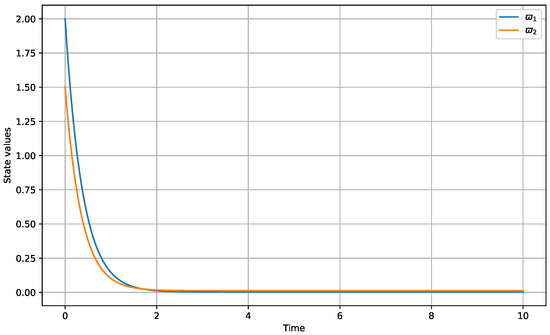
Figure 2. State trajectories for Example 2 with $\iota =0.8$, $\tau =0.6$, and $\beta =0.03$. The substate $({\varpi }_1,{\varpi }_2)$ shows exponential convergence to the stability ball.

4. Practical Stability for a Class of Triangular Systems

Let us consider the following TFOS:

$$\begin{array}{ccc}\hfill {}^{C}D_{{\omega }_0^{+}}^{\iota ,\tau }{\varpi }^1\left(\varkappa \right)& =& A{\varpi }^1+Bu+G_1(\varkappa ,{\varpi }^1,{\varpi }^2,u,\beta ),\hfill \end{array}$$

(36)

$$\begin{array}{ccc}\hfill {}^{C}D_{{\omega }_0^{+}}^{\iota ,\tau }{\varpi }^2\left(\varkappa \right)& =& G_2(\varkappa ,{\varpi }^2,\beta ),\varkappa \ge {\omega }_0,\hfill \end{array}$$

(37)

where ${\varpi }^1\in {\mathbb{R}}^{n_1},{\varpi }^2\in {\mathbb{R}}^{n_2}.$

Let us consider the following assumption:

$\left(H\right):$ For every $\varkappa \ge 0$, $\beta >0$, and ${\varpi }^1\in {\mathbb{R}}^{n_1}$, ${\varpi }^2\in {\mathbb{R}}^{n_2}$, $u\in {\mathbb{R}}^q$

$$\parallel G_1(\varkappa ,{\varpi }^1,{\varpi }^2,u,\beta )\parallel \le {\delta }_1\left(\beta \right)\phi \left(\varkappa \right)+{\delta }_2\left(\beta \right)\parallel {\varpi }^1\parallel +{\delta }_3\left(\beta \right)\parallel u\parallel ,$$

(38)

such that $\phi$ is a nonnegative continuous function, ${\delta }_1\left(\beta \right)>0,$${\delta }_2\left(\beta \right)>0$, ${\delta }_3\left(\beta \right)>0$, and ${\delta }_1\left(\beta \right),{\delta }_2\left(\beta \right),{\delta }_3\left(\beta \right)⟶0$ as $\beta ⟶0^{+}$.

Theorem 3.

Under assumption $\left(H\right)$, the system (36) and (37) with the feedback law $u=K{\varpi }^1$ is ${\beta }_1$-PUGMLS-${\varpi }^1$ for some ${\beta }_1>0$ if there exist $P=P^T>0$, $K\in {\mathbb{R}}^{m\times n_1}$, $ϵ>0$, and $\widetilde{ϵ}\in (0,ϵ)$ such that

$$S^{T}P+PS+ϵI<0,$$

(39)

with $S=A+BK$ and the function

$${\displaystyle \varkappa \mapsto {\int }_0^{\varkappa }{(\varkappa -l)}^{\iota -1}exp\left(-\tau (\varkappa -l)\right)E_{\iota ,\iota }\left(-\frac{(ϵ-\widetilde{ϵ})}{{\lambda }_{max}\left(P\right)}{(\varkappa -l)}^{\iota }\right){\phi }^2\left(l\right)dl}$$

is bounded.

Proof. 

We have from (39)

$$\begin{array}{cc}\hfill 2{{\varpi }^1}^{T}P{G}_1(\varkappa ,{\varpi }^1,{\varpi }^2,u,\beta )& \le 2\parallel {\varpi }^1\parallel \parallel P\parallel \parallel G_1(\varkappa ,{\varpi }^1,{\varpi }^2,u,\beta )\parallel \hfill \\ \hfill & \le 2\parallel {\varpi }^1\parallel \parallel P\parallel \left({\delta }_1\left(\beta \right)\phi \left(\varkappa \right)+{\delta }_2\left(\beta \right)\parallel {\varpi }^1\parallel +{\delta }_3\left(\beta \right)\parallel K\parallel \parallel {\varpi }^1\parallel \right).\hfill \end{array}$$

(40)

Let $0<{\widetilde{ϵ}}_1<\widetilde{ϵ},$ we have

$$2\parallel {\varpi }^1\parallel \parallel P\parallel {\delta }_1\left(\beta \right)\phi \left(\varkappa \right)\le {\widetilde{ϵ}}_1{\parallel {\varpi }^1\parallel }^2+{\displaystyle \frac{{\parallel P\parallel }^2{\delta }_1{\left(\beta \right)}^2{\phi }^2\left(\varkappa \right)}{{\widetilde{ϵ}}_1}}.$$

(41)

Therefore,

$$2{{\varpi }^1}^{T}P{G}_1(\varkappa ,{\varpi }^1,{\varpi }^2,u,\beta )\le \left({\widetilde{ϵ}}_1+2{\delta }_2\left(\beta \right)\parallel P\parallel +2{\delta }_3\left(\beta \right)\parallel P\parallel \parallel K\parallel \right){\parallel {\varpi }^1\parallel }^2+{\displaystyle \frac{{\parallel P\parallel }^2{\delta }_1{\left(\beta \right)}^2{\phi }^2\left(\varkappa \right)}{{\widetilde{ϵ}}_1}}.$$

Since ${\displaystyle \underset{\beta \to 0}{lim}{\delta }_2\left(\beta \right)=0}$ and ${\displaystyle \underset{\beta \to 0}{lim}{\delta }_3\left(\beta \right)=0}$, then there is ${\beta }_1>0$ such that for each $\beta \in (0,{\beta }_1]$, we get

$$2{{\varpi }^1}^{T}P{G}_1(\varkappa ,{\varpi }^1,{\varpi }^2,u,\beta )\le \widetilde{ϵ}{\parallel {\varpi }^1\parallel }^2+{\displaystyle \frac{{\parallel P\parallel }^2{\delta }_1{\left(\beta \right)}^2{\phi }^2\left(\varkappa \right)}{{\widetilde{ϵ}}_1}}.$$

(42)

Let $\beta \in (0,{\beta }_1]$ and $V(\varkappa ,{\varpi }^1,{\varpi }^2)={{\varpi }^1}^{T}P{\varpi }^1$.

We get

$$\begin{array}{cc}\hfill {}^{C}D_{{\omega }_0^{+}}^{\iota ,\tau }{V}_{\beta }(\varkappa ,{\varpi }_{\beta }(\varkappa ;{\omega }_0,{\varpi }_0))& \le 2{\varpi }^1{(\varkappa ;{\omega }_0,{\varpi }_0)}^T{P}^C{D}_{{\omega }_0^{+}}^{\iota ,\tau }{\varpi }^1(\varkappa ;{\omega }_0,{\varpi }_0)\hfill \\ \hfill & \le {\varpi }^1{(\varkappa ;{\omega }_0,{\varpi }_0)}^T\left((S^{T}P+PS\right){\varpi }^1(\varkappa ;{\omega }_0,{\varpi }_0)\hfill \\ \hfill & +2{\varpi }^1{(\varkappa ;{\omega }_0,{\varpi }_0)}^{T}P{G}_1(\varkappa ,{\varpi }^1,{\varpi }^2,u,\beta ).\hfill \end{array}$$

(43)

Using (39), (42), and (43), we get

$${}^{C}D_{{\omega }_0^{+}}^{\iota ,\tau }{V}_{\beta }(\varkappa ,{\varpi }_{\beta }(\varkappa ;{\omega }_0,{\varpi }_0))\le -R{\parallel {\varpi }^1(\varkappa ;{\omega }_0,{\varpi }_0)\parallel }^2+{\displaystyle \frac{{\parallel P\parallel }^2{\delta }_1{\left(\beta \right)}^2{\phi }^2\left(\varkappa \right)}{{\widetilde{ϵ}}_1}},$$

with $R=ϵ-\widetilde{ϵ}.$

Therefore, all hypotheses of Theorem 1 hold, and then the system (36) and (37) with the feedback law $u=K{\varpi }^1$ is ${\beta }_1$-PUGMLS-${\varpi }^1$ for some ${\beta }_1>0$. □

Example 3.

Let the following TFOS

$$\begin{array}{cc}{}^{C}D_{{\omega }_0^{+}}^{\iota ,\tau }{\varpi }_1\hfill & =-{\varpi }_1+{\varpi }_2+{\displaystyle \frac{3}{2}}u+{\displaystyle \frac{1}{2}}{\beta }^{2}sin\left(u\right)sin\left({\varpi }_1\right),\hfill \\ {}^{C}D_{{\omega }_0^{+}}^{\iota ,\tau }{\varpi }_2\hfill & ={\varpi }_2+u+{\displaystyle \frac{1}{6}}{\beta }^{2}cos\left({\varpi }_3\right),\hfill \\ {}^{C}D_{{\omega }_0^{+}}^{\iota ,\tau }{\varpi }_3\hfill & ={\varpi }_3,\hfill \end{array}$$

(44)

with $\varpi =\left({\varpi }_1,{\varpi }_2,{\varpi }_3\right)\in {\mathbb{R}}^3$.

This system has the same form of system (36) and (37) with

$$A=\left(\begin{array}{cc}-1& 1\\ 0& 1\end{array}\right),$$

$$B=\left(\begin{array}{c}{\displaystyle \frac{3}{2}}\\ 1\end{array}\right)$$

and

$$G_1(\varkappa ,\varpi ,u,\beta )={\displaystyle \frac{1}{2}}{\beta }^{2}sin\left(u\right)(sin({\varpi }_1),0,0)+(0,{\displaystyle \frac{1}{6}}{\beta }^{2}cos\left({\varpi }_3\right),0).$$

The perturbed term $G_1$ satisfies $\left(H\right)$ with ${\delta }_1\left(\beta \right)={\displaystyle \frac{1}{6}}{\beta }^2$, ${\delta }_2\left(\beta \right)={\displaystyle \frac{1}{2}}{\beta }^2$, ${\delta }_3\left(\beta \right)=0$, and $\phi \left(\varkappa \right)=1$.

The condition (39) is satisfied for $ϵ=1$, $P=I$, and $K=\left(\begin{array}{cc}0& -2\end{array}\right).$

Then, by using the previous theorem, we get the ${\beta }^{*}$-PUGMLS-$({\varpi }_1,{\varpi }_2)$ for TFOS (44).

Interpretation: The proposed feedback controller $u=K{\varpi }^1$ effectively stabilizes the triangular system described in Example 3. As shown in Figure 3, the substate $({\varpi }_1,{\varpi }_2)$ converges to the desired ball of radius 0.01 despite the presence of nonlinear perturbations. Figure 4 shows the control effort, which is reasonable and converges to zero as the system stabilizes. This demonstrates the practical applicability of the theoretical controller design methodology.

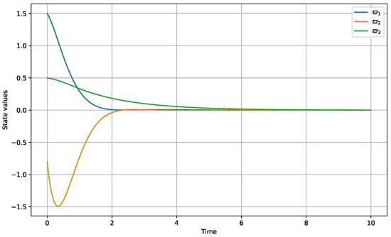
Figure 3. Closed-loop system trajectories for Example 3 with $\iota =0.6$, $\tau =0.4$, and $\beta =0.1$. The controller successfully stabilizes the substate $({\varpi }_1,{\varpi }_2)$.

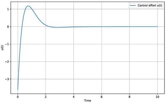
Figure 4. Control effort for the stabilization of the Example 3 system.

Theorem 4.

Under assumption $\left(H\right)$, the system (36) and (37) with the feedback law $u=K{\varpi }^1$ is ${\beta }_1$-PUES-${\varpi }^1$ for some ${\beta }_1>0$ if there exist $P=P^T$, $K\in {\mathbb{R}}^{m\times n_1}$, $\tilde{a}\in [0,{\tau }^{\iota })$, $ϵ\in \mathbb{R}$, and $\widetilde{ϵ}>0$ such that

$$S^{T}P+PS-ϵI<0\mathrm{with}S=A+BK,$$

(45)

$$0\le {\displaystyle \frac{ϵ+\widetilde{ϵ}}{{\lambda }_{min}\left(P\right)}}\le \tilde{a}$$

(46)

and the function

$${\displaystyle \varkappa \mapsto {\int }_0^{\varkappa }{(\varkappa -w)}^{\iota -1}{E}_{\iota ,\iota }\left(\tilde{a}{(\varkappa -w)}^{\iota }\right)exp\left(-\tau (\varkappa -w)\right){\phi }^2\left(w\right)dw}$$

is bounded.

Proof. 

Let $0<{\widetilde{ϵ}}_1<\widetilde{ϵ}$. Similar to the proof of Theorem 3, we get

$$2{{\varpi }^1}^{T}P{G}_1(\varkappa ,{\varpi }^1,{\varpi }^2,u,\beta )\le \left({\widetilde{ϵ}}_1+2{\delta }_2\left(\beta \right)\parallel P\parallel +2{\delta }_3\left(\beta \right)\parallel P\parallel \parallel K\parallel \right){\parallel {\varpi }^1\parallel }^2+{\displaystyle \frac{{\parallel P\parallel }^2{\delta }_1{\left(\beta \right)}^2{\phi }^2\left(\varkappa \right)}{{\widetilde{ϵ}}_1}}.$$

Since ${\displaystyle \underset{\beta \to 0}{lim}{\delta }_2\left(\beta \right)=0}$ and ${\displaystyle \underset{\beta \to 0}{lim}{\delta }_3\left(\beta \right)=0}$, then there is ${\beta }_1>0$ such that for each $\beta \in (0,{\beta }_1]$, we get

$$2{{\varpi }^1}^{T}P{G}_1(\varkappa ,{\varpi }^1,{\varpi }^2,u,\beta )\le \widetilde{ϵ}{\parallel {\varpi }^1\parallel }^2+{\displaystyle \frac{{\parallel P\parallel }^2{\delta }_1{\left(\beta \right)}^2{\phi }^2\left(\varkappa \right)}{{\widetilde{ϵ}}_1}}.$$

(47)

Let $\beta \in (0,{\beta }_1]$ and $V(\varkappa ,{\varpi }^1,{\varpi }^2)={{\varpi }^1}^{T}P{\varpi }^1$.

We get

$$\begin{array}{cc}\hfill {}^{C}D_{{\omega }_0^{+}}^{\iota ,\tau }{V}_{\beta }(\varkappa ,{\varpi }_{\beta }(\varkappa ;{\omega }_0,{\varpi }_0))& \le 2{\varpi }^1{(\varkappa ;{\omega }_0,{\varpi }_0)}^T{P}^C{D}_{{\omega }_0^{+}}^{\iota ,\tau }{\varpi }^1(\varkappa ;{\omega }_0,{\varpi }_0)\hfill \\ \hfill & \le {\varpi }^1{(\varkappa ;{\omega }_0,{\varpi }_0)}^T\left((S^{T}P+PS\right){\varpi }^1(\varkappa ;{\omega }_0,{\varpi }_0)\hfill \\ \hfill & +2{\varpi }^1{(\varkappa ;{\omega }_0,{\varpi }_0)}^{T}P{G}_1(\varkappa ,{\varpi }^1,{\varpi }^2,u,\beta ).\hfill \end{array}$$

(48)

Using (45), (47), and (48), we get

$${}^{C}D_{{\omega }_0^{+}}^{\iota ,\tau }{V}_{\beta }(\varkappa ,{\varpi }_{\beta }\left(\varkappa \right))\le R{\parallel {\varpi }^1(\varkappa ;{\omega }_0,{\varpi }_0)\parallel }^2+{\displaystyle \frac{{\parallel P\parallel }^2{\delta }_1{\left(\beta \right)}^2{\phi }^2\left(\varkappa \right)}{{\widetilde{ϵ}}_1}},$$

with $R=ϵ+\widetilde{ϵ}.$

Therefore, all hypotheses of Theorem 2 hold, then the system (36) and (37) with the feedback law $u=K{\varpi }^1$ is ${\beta }_1$-PUES-${\varpi }^1$ for some ${\beta }_1>0$. □

Example 4.

Let the following TFOS

$$\begin{array}{cc}{}^{C}D_{{\omega }_0^{+}}^{\iota ,\tau }{\varpi }_1\hfill & =-{\displaystyle \frac{1}{2}}{\varpi }_1+3{\varpi }_2+u+{\displaystyle \frac{1}{3}}\beta cos\left({\varpi }_3\right),\hfill \\ {}^{C}D_{{\omega }_0^{+}}^{\iota ,\tau }{\varpi }_2\hfill & =2{\varpi }_2+{\displaystyle \frac{5}{2}}u+{\displaystyle \frac{1}{5}}\beta sin\left({\varpi }_2\right),\hfill \\ {}^{C}D_{{\omega }_0^{+}}^{\iota ,\tau }{\varpi }_3\hfill & =2{\varpi }_3,\hfill \end{array}$$

(49)

with $\varpi =\left({\varpi }_1,{\varpi }_2,{\varpi }_3\right)\in {\mathbb{R}}^3$.

This system has the same form of (36) and (37) with

$$A=\left(\begin{array}{cc}-2& 3\\ 0& 2\end{array}\right),$$

$$B=\left(\begin{array}{c}1\\ {\displaystyle \frac{5}{2}}\end{array}\right)$$

and

$$G_1(\varkappa ,\varpi ,u,\beta )={\displaystyle \frac{1}{3}}\beta cos({\varpi }_3)(1,0,0)+(0,{\displaystyle \frac{1}{5}}\beta sin\left({\varpi }_2\right),0).$$

The perturbed term $G_1$ satisfies $\left(H\right)$ with ${\delta }_1\left(\beta \right)={\displaystyle \frac{1}{3}}\beta$, ${\delta }_2\left(\beta \right)={\displaystyle \frac{1}{5}}\beta$, ${\delta }_3\left(\beta \right)=0$, and $\phi \left(\varkappa \right)=1$.

The condition (45) is satisfied for $ϵ=-{\displaystyle \frac{1}{2}}$, $\widetilde{ϵ}={\displaystyle \frac{1}{2}}$, $\tilde{a}=0,$$P=I$, and $K=\left(\begin{array}{cc}0& -1\end{array}\right).$

Then, by using the previous Theorem, we get the ${\beta }^{*}$-PUES-$({\varpi }_1,{\varpi }_2)$ for TFOS (49).

Interpretation: The simulation results for Example 4, presented in Figure 5 and Figure 6, validate the ${\beta }^{*}$-PUES property for the controlled system. The substate $({\varpi }_1,{\varpi }_2)$ converges exponentially to the ball of radius 0.01. Figure 6 demonstrates the system’s robustness to variations in the parameter $\beta$, with smaller values of $\beta$ leading to better convergence properties (smaller ultimate bounds), as predicted by the theory.

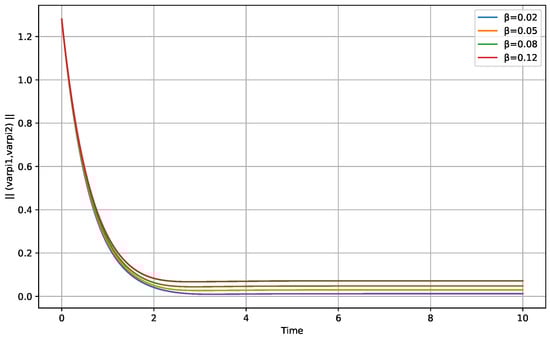
Figure 5. State trajectories for Example 4 with $\iota =0.9$, $\tau =0.7$, and $\beta =0.08$. The controlled substate $({\varpi }_1,{\varpi }_2)$ shows practical uniform exponential stability.

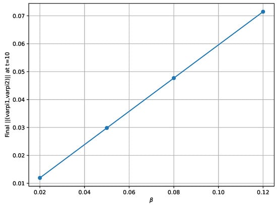
Figure 6. Robustness analysis showing system performance under different $\beta$ values.

5. Conclusions

This paper has established a comprehensive Lyapunov-based framework for analyzing partial practical stability in nonlinear TFOS. We have introduced and rigorously analyzed two novel stability concepts, ${\beta }^{*}$-PUGMLS and ${\beta }^{*}$-PUES, with respect to system substates. Through the development of appropriate Lyapunov functions and inequality techniques, we derived sufficient conditions that guarantee the convergence of system states to a predefined neighborhood of the origin.

The theoretical contributions include the extension of classical stability theory to tempered fractional calculus systems, providing both Mittag–Leffler and exponential stability criteria that account for the tempered parameter’s influence on system behavior. Furthermore, we successfully applied these stability results to design effective feedback controllers for a class of triangular TFOS, demonstrating the practical applicability of our theoretical developments. The presented examples have validated the effectiveness of our stability criteria and control strategies, showing consistent convergence behavior under various system configurations and parameter variations. This work not only advances the theoretical understanding of stability in tempered fractional-order systems but also provides practical tools for controlling complex nonlinear systems in engineering applications.

Future research will focus on several promising extensions of this work. First, the development of adaptive control strategies is a natural next step, which would allow the controller parameters to self-tune in response to unknown system uncertainties or time-varying perturbations, enhancing the robustness of the proposed framework. Second, the design of state observers for TFOS is critical for practical implementations, where not all system states are measurable; extending our results to output-feedback control using observer-based designs would significantly broaden the applicability of the method. Furthermore, exploring these stability and control techniques with new fractional operators, such as the ones containing non-singular kernels or variable orders, could yield even more accurate modeling and control capabilities. Finally, applying this theoretical framework to complex real-world systems in fields such as power systems, mechanical engineering, and biomedical engineering will be a key direction, leveraging the enhanced accuracy that tempered fractional models provide for systems with memory and anomalous diffusion phenomena.

References

- Dorgham, A.; Hammami, M.A. Practical tracking control of a class of uncertain nonlinear systems and unknown output function. Int. J. Adapt. Control Signal Process. 2023, 37, 2434–2450. [Google Scholar] [CrossRef]
- Damak, H.; Hammami, M.A.; Maaloul, K. Observers Based Control for Stabilization of Non-autonomous Evolution Equations in Banach Spaces. Complex Anal. Oper. Theory 2023, 17, 65. [Google Scholar] [CrossRef]
- Ben Makhlouf, A. On the Stability of Caputo Fractional-Order Systems: A Survey. In Fractional Order Systems-Control Theory and Applications: Fundamentals and Applications; Springer International Publishing: Cham, Switzerland, 2021; pp. 1–8. [Google Scholar]
- Sontag, E.D. Smooth stabilization implies coprime factorization. IEEE Trans. Autom. Control 1989, 34, 435–443. [Google Scholar] [CrossRef]
- El-Borai, M.M.; Moustafa, O.L.; Ahmed, H.M. Asymptotic stability of some stochastic evolution equations. Appl. Math. Comput. 2003, 144, 273–286. [Google Scholar] [CrossRef]
- Khandani, K.; Majd, M.J.; Tahmasebi, M. Integral sliding mode control for robust stabilisation of uncertain stochastic time-delay systems driven by fractional Brownian motion. Int. J. Syst. Sci. 2017, 48, 828–837. [Google Scholar] [CrossRef]
- Benabdallah, A.; Ellouze, I.; Hammami, M.A. Practical exponential stability of perturbed triangular systems and a separation principle. Asian J. Control 2011, 13, 445–448. [Google Scholar] [CrossRef]
- Ghanmi, B. On the Practical h-stability of Nonlinear Systems of Differential Equations. J. Dyn. Control Syst. 2019, 25, 691–713. [Google Scholar] [CrossRef]
- Hamzaoui, A.; Taieb, N.H.; Hammami, M.A. Practical partial stability of time-varying systems. Discret. Contin. Dyn.-Syst.-B 2022, 7, 3585–3603. [Google Scholar] [CrossRef]
- Ghanmi, B. Stability of impulsive systems depending on a parameter. Math. Methods Appl. Sci. 2016, 39, 2626–2646. [Google Scholar] [CrossRef]
- Alaia, E.B.; Dhahri, S.; Naifar, O. A Gradient-Based Optimization Algorithm for Optimal Control Problems with General Conformable Fractional Derivatives. IEEE Access 2025, 2025, 3595958. [Google Scholar] [CrossRef]
- Naifar, O. Practical Observer Design for Nonlinear Systems using Caputo Fractional Derivative with Respect to Another Function. In Proceedings of the IEEE 22nd International Multi-Conference on Systems, Signals and Devices (SSD), Monastir, Tunisia, 17–20 February 2025; pp. 411–418. [Google Scholar]
- Naifar, O.; Makhlouf, A.B.; Mchiri, L.; Rhaima, M. Finite Time Stability for Hadamard Fractional-Order Systems. Ain Shams Eng. J. 2025, 16, 103263. [Google Scholar] [CrossRef]
- Dhahri, S.; Naifar, O. Fault-Tolerant Tracking Control for Linear Parameter-Varying Systems under Actuator and Sensor Faults. Mathematics 2023, 11, 4738. [Google Scholar] [CrossRef]
- Dhahri, S.; Naifar, O. Robust Fault Estimation and Tolerant Control for Uncertain Takagi-Sugeno Fuzzy Systems. Symmetry 2023, 15, 1894. [Google Scholar] [CrossRef]
- Ben Makhlouf, A.; Naifar, O. On the Barbalat Lemma Extension for the Generalized Conformable Fractional Integrals: Application to Adaptive Observer Design. Asian J. Control 2023, 25, 563–569. [Google Scholar]
- Naifar, O.; Boukettaya, G. On Observer Design of Systems Based on Renewable Energy. In Advances in Observer Design and Observation for Nonlinear Systems: Fundamentals and Applications; Springer: Cham, Switzerland, 2022; pp. 135–176. [Google Scholar]
- Naifar, O.; Makhlouf, A.B. Synchronization of Mutual Coupled Fractional Order One-Sided Lipschitz Systems. Integration 2021, 80, 41–45. [Google Scholar] [CrossRef]
- Naifar, O.; Jmal, A.; Ben Makhlouf, A.; Derbel, N.; Hammami, M.A. Fault Estimation for Nonlinear One-Sided Lipschitz Systems. In Fractional Order Systems—Control Theory and Applications: Fundamentals and Applications; Springer: Cham, Switzerland, 2021; pp. 95–122. [Google Scholar]
- Naifar, O.; Jmal, A.; Ben Makhlouf, A.; Derbel, N.; Hammami, M.A. Observer-Based Control for Fractional-Order Systems. In Fractional Order Systems—Control Theory and Applications: Fundamentals and Applications; Springer: Cham, Switzerland, 2021; pp. 75–93. [Google Scholar]
- Engheta, N. On fractional calculus and fractional multipoles in electromagnetism. IEEE Trans. Antennas Propag. 1996, 44, 554–566. [Google Scholar] [CrossRef]
- Hilfer, R. Applications of Fractional Calculus in Physics; World Scientific: Singapore, 2000. [Google Scholar]
- Sadek, L.; Sadek, O.; Alaoui, H.T.; Abdo, M.S.; Shah, K.; Abdeljawad, T. Fractional order modeling of predicting covid-19 with isolation and vaccination strategies in Morocco. CMES-Comput. Model. Eng. Sci 2023, 136, 1931–1950. [Google Scholar] [CrossRef]
- Erturk, V.S.; Kumar, P. Solution of a COVID-19 model via new generalized Caputo-type fractional derivatives. Chaos Solitons Fractals 2020, 139, 110280. [Google Scholar] [CrossRef]
- Ben Makhlouf, A. Superstability of higher-order fractional differential equations. Ann. Univ. Craiova-Math. Comput. Sci. Ser. 2022, 49, 11–14. [Google Scholar]
- Rguigui, H.; Elghribi, M. Practical stabilization for a class of tempered fractional-order nonlinear fuzzy systems. Asian J. Control 2025. [Google Scholar] [CrossRef]
- Gassara, H.; Kharrat, D.; Ben Makhlouf, A.; Mchiri, L.; Rhaima, M. SOS Approach for Practical Stabilization of Tempered Fractional-Order Power System. Mathematics 2023, 11, 3024. [Google Scholar] [CrossRef]
- Ben Makhlouf, A. Stability with respect to part of the variables of nonlinear Caputo fractional differential equations. Math. Commun. 2018, 23, 119–126. [Google Scholar]
- Ben Makhlouf, A. Partial practical stability for fractional-order nonlinear systems. Math. Methods Appl. Sci. 2022, 45, 5135–5148. [Google Scholar] [CrossRef]
- Ben Makhlouf, A. A novel finite time stability analysis of nonlinear fractional-order time delay systems: A fixed point approach. Asian J. Control 2022, 24, 3580–3587. [Google Scholar] [CrossRef]
- Naifar, O. Tempered Fractional Gradient Descent: Theory, Algorithms, and Robust Learning Applications. Neural Netw. 2025, 193, 108005. [Google Scholar] [CrossRef] [PubMed]
- Abouelregal, A.E.; Alhassan, Y.; Alsaeed, S.S.; Elzayady, M.E. Tempered Fractional Thermal Conduction Model for Magnetoelastic Solids with Spherical Holes under Time-Dependent Laser Pulse Heating. Arch. Appl. Mech. 2025, 95, 27. [Google Scholar] [CrossRef]
- Abouelregal, A.E.; Civalek, Ö; Akgöz, B.; Foul, A.; Askar, S.S. Analysis of Thermoelastic Behavior of Porous Cylinders with Voids via a Nonlocal Space-Time Elastic Approach and Caputo-Tempered Fractional Heat Conduction. Mech. Time-Depend. Mater. 2025, 29, 1–32. [Google Scholar] [CrossRef]
- Alawad, M.A.; Louhichi, B. Innovative Observer Design for Nonlinear Tempered Fractional-Order Systems. Asian J. Control 2025. [Google Scholar] [CrossRef]
- Deng, J.; Ma, W.; Deng, K.; Li, Y. Tempered Mittag-Leffler Stability of Tempered Fractional Dynamical Systems. Math. Probl. Eng. 2020, 2020, 7962542. [Google Scholar] [CrossRef]
- Kilbas, A.A.; Srivastava, H.M.; Trujillo, J.J. Theory and Applications of Fractional Differential Equations; North-Holland Mathematics Studies; Elsevier: Amsterdam, The Netherlands, 2006; Volume 204. [Google Scholar]
- Erdelyi, A. Higher Transcendental Functions; McGraw-Hill: New-York, NY, USA, 1953; Volume III. [Google Scholar]
- Podlubny, I. Fractional Differential Equations; Academic Press: San Diego, CA, USA, 1999. [Google Scholar]
- Miller, K.; Samko, S. A Note on the Complete Monotonicity of the Generalized Mittag-Leffler Function. Real Anal. Exch. 1999, 23, 753–756. [Google Scholar] [CrossRef]
- Kuczma, M. An Introduction to the Theory of Functional Equations and Inequalities: Cauchy’s Equation and Jensen’s Inequality; Birkhauser: Basel, Switzerland, 2009. [Google Scholar]
- Li, C.; Deng, W.; Zhao, L. Well-posedness and numerical algorithm for the tempered fractional differential equations. Discret. Contin. Dyn. Syst. Ser. B 2019, 24, 1989–2015. [Google Scholar] [CrossRef]
- Miller, R.K.; Feldstein, A. Smoothness of solutions of Volterra integral equations with weakly singular kernels. SIAM J. Math. Anal. 1971, 2, 242–258. [Google Scholar] [CrossRef]
Disclaimer/Publisher’s Note: The statements, opinions and data contained in all publications are solely those of the individual author(s) and contributor(s) and not of MDPI and/or the editor(s). MDPI and/or the editor(s) disclaim responsibility for any injury to people or property resulting from any ideas, methods, instructions or products referred to in the content. |
© 2025 by the author. Licensee MDPI, Basel, Switzerland. This article is an open access article distributed under the terms and conditions of the Creative Commons Attribution (CC BY) license (https://creativecommons.org/licenses/by/4.0/).