On Estimation of α-Stable Distribution Using L-Moments

Abstract

The family of stable distributions and, in particular, the $\alpha$-stable distribution increases its applicability in engineering sciences. Examination of industrial data shows that originally assumed Gaussian properties are not so often observed. Research shows that stable functions can cover much wider spectrum of cases. However, the estimations of $\alpha$-stable distribution factors may pose some limitations. One of the control engineering aspects, i.e., the assessment of controller performance, may be successfully addressed by L-moments and L-moment ratio diagrams (LMRD). Simultaneously, LMRDs are often used as a method for distribution, fitting with the method of moments (MOM). Unfortunately, the moments do not exist for $\alpha$-stable distribution. This research shows that, with the use of a Monte-Carlo analysis, this limitation may be overcome, and an efficient method to estimate statistical factors of the $\alpha$-stable distribution is proposed.

1. Introduction

This paper addresses an important aspect of heavy tail modeling. Heavy tails, though underestimated, occur frequently in real life. The story of tails is inevitably connected to the notion of outliers. Outliers, anomalies, oddities, discordant observations, contamination, deviants, exceptions, or aberrations represent “unusual events that occur more often than seldom” [1]. They appear more than frequently because of various, mostly unknown reasons. Historically, statisticians have encountered, identified, and analyzed them first. Real data observations enable the modeling of fundamental stochastic processes. Probabilistic density distributions play an important role role, as the assessment of their properties makes it possible to extrapolate our knowledge.

Heavy tails can be successfully used to describe such phenomena. They may mean that a given distribution follows the power law. In other cases, they mean that it is scale-free. They may refer to stable or subexponential distributions, or they witness an infinite variance. Actually, a given distribution is heavy-tailed if its tail is heavier than any exponential distribution [2]. Detailed explanations may be found in [3].

Stochastic data analysis allows us to identify and model tails. However, this is only one side of the coin. Abnormal observations and tails are closely interconnected with other data interpretations and various phenomena, such as persistence [4], fractality [5,6], Hurst exponent [7], and fractionality [8]. Stable functions, and especially $\alpha$-stable distribution, allows for addressing that issue efficiently through the existence of the stability exponent $\alpha$.

This work addresses the heavy-tailed properties of the $\alpha$-stable distribution and its detection. These features are closely connected to fractionality, though it has a different name and is assessed from a statistical perspective.

The problem of how to fit an unknown PDF function to the experimental data is well-known. The problem consists of two elements: a choice of the function itself and an estimation of its coefficients. This problem can be addressed separately or together. One may utilize different approaches [9], like distribution function fitting to the histogram, method of moments, quantile Q-Q plots, or L-moment ratio diagrams [10,11]. Each method has its scope of applicability and exhibits certain properties.

Apart from probabilistic distributions and their factors, statistics deliver alternative formulations of moments. Recent research by [9,12] shows that L-moments, which were proposed by [13], can play the role of the PDF fitting mechanisms [14]. They are successfully used not only in extreme data analysis [15,16] but also in economics [17] or control engineering [18].

L-moments exhibit a lot of advantages, as they are analog to conventional moment estimates: shift, scale, skewness, and kurtosis. They introduce new characterization of the PDF shape and help to estimate its factors [19]. Similarly to the method of moments, this is achieved by fitting the empirical L-moments to the exact theoretical values. We may evaluate them theoretically for many distributions, but the moments must exist. As the theoretical moments of the $\alpha$-stable distribution may not exist, which depends on its parametrization, we cannot apply it directly [20].

This paper presents original solution to an open problem of fitting stable probabilistic density function (PDF) to experimental data for distributions with non-existent moments. This task is solved using L-moment ratio diagrams (LMRD). The most challenging aspect of this work is the utilization of Monte-Carlo approach that allows for addressing the challenge of using a method of moments in case of infinite moments of $\alpha$-stable distribution. It is shown that, by recurring estimations, we may identify polynomial curves in the LMRD diagram that relate to the factors of the $\alpha$-stable distribution, but the estimation quality depends on stability exponent and its skewness.

The description starts with Section 2, which describes used methodology and algorithms. It allows for further formulation of $\alpha$-stable estimation experiments in Section 3. Section 4 concludes the paper and shows areas for further research.

2. Methods and Algorithms

This section describes applied methods and algorithms. It starts with the formulation of $\alpha$-stable distribution function and is followed by descriptions of PDF fitting, L-moments, and L-moment ratio diagrams.

2.1. The $\alpha$-Stable Distribution

Probability density function is a mathematical concept widely utilized in statistics. It serves as a tool to describe the probability distribution of a random variable, providing insights into the likelihood of different values that the variable may take on. The PDF, typically denoted as $\mathcal{F}\left(x\right)$, characterizes the probability density of a random variable X, taking a specific value x. For any interval $\left(a, b\right)$, the probability of X falling within that interval is determined by integrating the PDF over that range:

$$P\left(a<X<b\right)={\int }_a^a\mathcal{F}\left(x\right)dx.$$

(1)

Research [21] shows that $\mathcal{F}\left(x\right)$ adheres to two fundamental conditions:

−

Non-negativity: $\mathcal{F}\left(x\right)\ge 0$ for all x, which ensures its non-negativity;

−

Normalization: the integral of $\mathcal{F}\left(x\right)$ over the entire range equals 1 as follows:

$${\int }_{-\infty }^{\infty }\mathcal{F}\left(x\right)dx=1.$$

(2)

The family of stable distributions, and specifically the $\alpha$-stable function, constitutes an alternative and an extension to normal distribution. For identically distributed and independent random variables $x_1,x_2,\dots ,x_n$ and X, the data X is said to follow an $\alpha$-stable distribution, if there exists a real number $D_n$ and a positive constant $C_n$ that the relation satisfies:

$$X_1+X_2+\cdots +X_n\stackrel{d}{=}{C}_n·X+D_n,$$

(3)

where $\stackrel{d}{=}$ means equality in distribution. The $\alpha$-stable function cannot be described in a closed probabilistic density function formulation, and we express it with its characteristics equation:

$${\mathcal{F}}_{\alpha ,\beta ,\delta ,\gamma }^{\mathrm{stab}}\left(x\right)=exp\left\{i\delta x-{\left|\gamma x\right|}^{\alpha }\left(1+i\beta {\displaystyle \frac{x}{\left|x\right|}}l\left(x,\alpha \right)\right)\right\},$$

(4)

where

$$l\left(x,\alpha \right)=\left\{\begin{array}{cc}tan\left({\displaystyle \frac{\pi \alpha }{2}}\right)\hfill & \mathrm{for}\alpha \ne 1\hfill \\ -{\displaystyle \frac{2}{\pi }}ln\left|x\right|\hfill & \mathrm{for}\alpha =1\hfill \end{array}\right..$$

$\delta \in \mathbb{R}$ is a distribution shift, $\gamma \ge 0$ a scale, $\left|\beta \right|\le 1$ a skewness coefficient, and $0<\alpha \le 2$ its index of stability or stability exponent. Therefore, the function exhibits four degrees of freedom with one shift, one scale, and two shape factors. Shift $\delta$ reflects a PDF position, but we should not confuse it with a mean estimator. Scaling $\gamma$ measures fluctuations of a given variable and informs about the distribution broadness. Coefficient $\beta$ reflects distribution skewness (asymmetry). The second shape factor, i.e., the stability index $\alpha$, is responsible for shape of a distribution tails; it reflects a tail’s heaviness. The smaller the $\alpha$ is, the heavier the tails we observe.

The literature shows that the second and higher moments do not exist for $\alpha <2$ [20]. We observe certain special cases with closed PDF forms:

−

For $\alpha =2$, we obtain independent realizations; specifically, for $\alpha =2$ and $\beta =0$, we obtain the exact normal distribution $\mathrm{N}\left(\delta ,\sqrt{2}\gamma \right)$, where ${\sigma }^2=2{\gamma }^2$;

−

$\alpha =1$ and $\beta =0$ reflect the Cauchy PDF;

−

$\alpha =0.5$ and $\beta =1$ a Lévy PDF;

−

$\alpha =1$ and $\beta =1$ a Landau PDF;

−

$\alpha ={\displaystyle \frac{3}{2}}$ and $\beta =0$ a Holtsmark PDF.

In case of a zero skewness $\beta =0$, we obtain the a symmetric $\alpha$-stable distribution, called S$\alpha$S. The fact of an infinite variance is not anything wrong, and it should not eliminate such PDFs from control research. Moreover, it is shown that many statistical processes are characterized by the infinite variance, while its mean deviations may be finite and well behaved [6].

Research in [22] shows that $\alpha$-stable function factors may be estimated in many ways, like by an iterative [23] approach based on the characteristics function estimation, a fast but not very accurate quantiles algorithm proposed by [24], the logarithmic moments method presented by [25], or the maximum likelihood (ML) approach [26], which achieves the highest accuracy but at the highest calculation cost. Recent research delivers new approaches, like multivariate method of moments [27], its recursive variants [28] or using a Gaussian kernel density distribution estimator [29]. Some methods allow for estimating only the stability index $\alpha$ [30,31]. The Koutrouvelis approach is used in this research, as it is a compromise between accuracy and calculation time.

The analysis of industrial data shows that $\alpha$-stable distribution may efficiently describe tailedness aspect of control problems. The reviews show that it works even better that normal distribution. The investigation of PID control systems [32] (overwhelming majority of industrial systems) or MPC-like predictive algorithms [4] shows the robustness of stable factors during the CPA task. This is reflected in simulation analyses and industrial applications as well.

2.2. Distribution Fitting

PDF fitting provides a mathematical method for modeling the underlying distribution of noisy data. By selecting appropriate distributions and evaluating their goodness of fit, it allows for a deeper understanding of the nature of noise signals. This process informs decision-making in noise signal modeling, simulation, and signal processing. By PDF fitting, the most suitable probabilistic model is identified, and signal properties are quantified.

The concept for a PDF function fitting to the histogram seems to be the most straightforward. It uses the idea [33] that the area under the histogram (area of the bins) should be equal to the area under a given distribution function. The procedure is quite straightforward. The method assumes that we know the distribution that we are fitting and we know how to estimate properly its factors analytically or using some estimation algorithm. The most frequent is a maximum likelihood (ML) estimation; however, the method may strictly depend on the distribution type.

Histogram fitting depends on the selected bin width. However, in case of relatively small widths, this influence diminishes. We have to be aware that this effect may also depend on selected distributions, as functions with more degrees of freedom might be more affected with bin selection. The method of moments (MoM) in its classical formulation requires the knowledge of moments, which is not achievable for some PDFs [34]. The $\alpha$-stable PDF constitutes such a case.

A quantile method uses the so called Q-Q plot, which represents values of the quantile function for empirical PDF estimated for given observations against theoretical quantiles in a ${\mathbb{R}}^2$ Cartesian coordinates. Let us assume that $\mathcal{F}\left(x\right)$ denotes some PDF, and $Q_{\mathrm{F}}\left(x\right)$ its quantile function. We denote the empirical quantile function using a generalized function based on the empirical PDF $Q_{\mathrm{e}}\left(x\right)=Q_{{\mathrm{F}}_e}\left(x\right)$. Thus, the Q-Q represents points $\left\{Q_{\mathrm{F}}\left(x\right),Q_{\mathrm{e}}\left(x\right)\right\}$ being a non-decreasing step function plotted as a scattered diagram. The PDF fitting with the Q-Q plot is based on the observation of the diagram linearity. The fitting performance for a given estimated function can be measured by the distance from a straight line of a perfect fit. We use Koutrouvelis’ approach, as it is a well-balanced compromise of accuracy and calculation time.

2.3. L-Moments

L-moments are proposed as linear combinations of order statistics [13]. The research on order statistics relates to the concept of statistics for ordered random variables and observations. Minimum, maximum, and median are the most common order statistics. L-moments constitute direct analogs to product moments, like mean, variance, skewness or kurtosis, but they are not numerically equivalent. We evaluate L-moments according to the following procedure. Firstly, in dataset $\left\{x\left(1\right),\dots ,x\left(N\right)\right\}$, N refers to the sample numbers, which are ranked in ascending order starting from 1 up to N. The L-moments ($l_1,\dots ,l_4$), the L-skewness ${\tau }_3$, and the L-kurtosis ${\tau }_4$ we calculate according to

$$l_1={\beta }_0,l_2=2{\beta }_1-{\beta }_0,$$

(5)

$$l_3=6{\beta }_2-6{\beta }_1+{\beta }_0,l_4=20{\beta }_3-30{\beta }_2+12{\beta }_1-{\beta }_0,$$

(6)

$${\tau }_3={\displaystyle \frac{l_3}{l_2}},{\tau }_4={\displaystyle \frac{l_4}{l_2}},$$

(7)

with

$${\beta }_j={\displaystyle \frac{1}{N}}\sum _{i=j+1}^N{x}_i{\displaystyle \frac{(i-1)(i-2)\cdots (i-j)}{(N-1)(N-2)\cdots (N-j)}}.$$

(8)

L-moments are equivalent to conventional moments. The first one denoted as $l_1$ is just an arithmetic mean. The second L-moment, called the L-scale $l_2$, reflects variable fluctuations. Apart of it, the dimensionless variant of the coefficient of variation exits [13] called L-Cv and derived as follows:

$$\mathrm{L}-\mathrm{Cv}={\tau }_2={\displaystyle \frac{l_2}{l_1}}.$$

(9)

Higher L-moments $l_3$ and $l_4$ relate to symmetry and concentration [13]. The rth order L-moment ratios [15] are defined as follows:

$${\tau }_r={\displaystyle \frac{l_r}{l_w}},r=3,4,5,\dots$$

(10)

The ${\tau }_3$ is knows as a sample L-skewness and the ${\tau }_4$ as L-kurtosis. Such estimators achieve the full range of population ratio values in opposition to the conventional formulations. They satisfy the condition $\left|{\tau }_r<1\right|$ and can measure, independently of a scale factor, the distribution shape. The L-skewness limits the L-kurtosis, as shown below:

$${\displaystyle \frac{1}{4}}\left(5{\tau }_3^2-1\right)\le {\tau }_4<1;{\displaystyle \frac{1}{4}}\le {\tau }_4<1.$$

(11)

Once the first moment for a given variable exists, then all higher L-moments also exist [13]. We may use a set of L-moments $\left\{l_1,l_2,{\tau }_3,{\tau }_4\right\}$ to characterize any univariate distribution. L-moments do not exist for PDFs that do not have finite means [35], like Cauchy, General Pareto, or variants of Generalized Extreme Value.

L-moments may improve conventional analyses. They introduce new distribution characterization and enable the estimate factors for a given PDF. We may do it by fitting the sample empirical L-moments to their exact theoretical formulations. Shape L-moments ${\tau }_3$ and ${\tau }_4$ are used as goodness-of-fit measures. Refs. [13,14,16] propose theoretical evaluations for various univariate distributions. Examples of basic univariate distributions are given in

Table 1. Theoretical values of ${\tau }_3$ and ${\tau }_4$ for selected univariate distributions.

	${\mathit{\tau }}_3$	${\mathit{\tau }}_4$
uniform	0.0	0.0
normal	0.0	0.1226
Laplace	0.0	17/22
EXP	1/3	1/6

. These values are used to describe respective points in the LMRD, which may be further used in data analysis or during the evaluation of data properties.

L-moments are subject to robust and almost unbiased estimation, even for small sample sizes [36]. They are less sensitive to outliers and tails. That allows for distributional analysis of various functions: normal and non-Gaussian; thin-tailed and heavy-tailed; symmetrical and skewed. Researchers use them in different tasks, like for regional frequency investigations [37], during homogeneity testing [11], or in discordant analysis [38].

2.4. Moment and L-Moment Ratio Diagrams

Moment ratio diagrams (MRDs), mentioned in [39], originated in the 19th century in Pearson’s investigations. They graphically present statistical data properties in a single two-dimensional plot. We can utilize them to measure the proximity between distributions, to show PDF versatility, to fit theoretical PDF to experimental data, to explain relationship between given PDFs, to classify distributions or to identify the homogeneity of given data [10].

The MRD displays a pair of moments in Cartesian coordinates. Generally, two variants are used [40]. The MRD(${\gamma }_3, {\gamma }_4$) diagram is mostly used. It draws the skewness ${\gamma }_3$ (or its square ${\gamma }_3^2$) as abscissa and kurtosis ${\gamma }_4$ as ordinate, drawn upside down. The chart presents moments pairs $\left\{{\gamma }_3, {\gamma }_4\right\}$, which a distribution attains. There exists theoretical area that limits the placement of moments pairs:

$${\gamma }_4-{\gamma }_3^2\ge 1.$$

(12)

Any distribution is represented by a point, a curve, or a region. It depends on a number of shape coefficients of the distribution. The function with no shape factors, like exponential, Gauss, or Laplace, is drawn as a single point. For normal PDF, it is $\left(0, 3\right)$, while for Laplace, it is $\left(0, 6\right)$.

A curve represents distributions parameterized by one shape factor, like lognormal (LGN), Student’s t-distribution, Weibull (WEI), or generalized Pareto (GPD). Regions address PDFs having two shape parameters, like a $\alpha$-stable or four-parameter kappa (K4D) distribution.

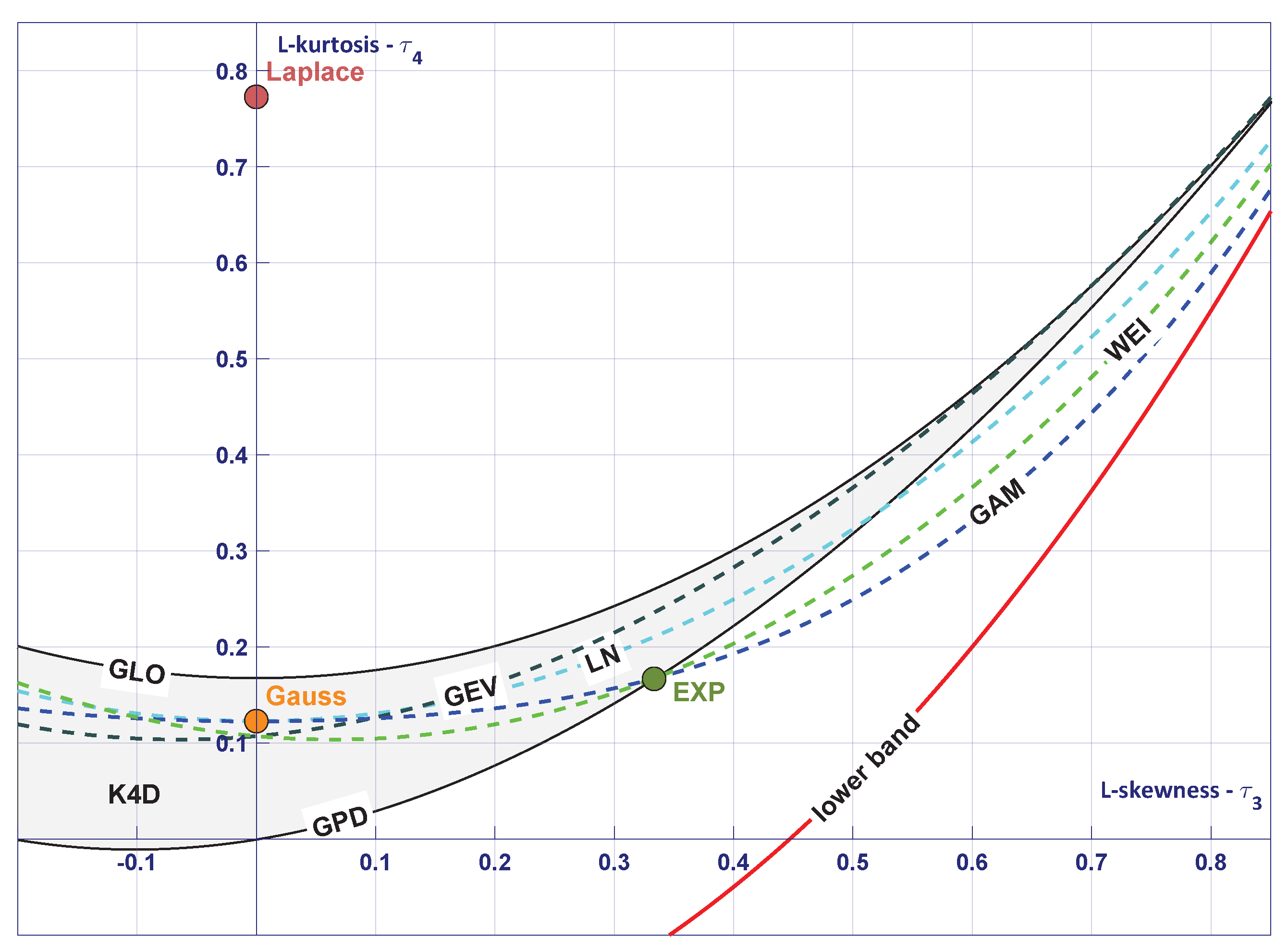
Another moment ratio diagram variant MRD(${\gamma }_2, {\gamma }_3$) compares skewness ${\gamma }_3$ as ordinate with variance ${\gamma }_2$ at abscissa [41]. It is shift- and scale-dependent. The utilization of MRD is very rare, contrary to its L-moment counterpart, i.e., L-moment ratio diagram. Similarly to MRDs, it applies to the PDF fitting [36]. The common diagram is the LMRD(${\tau }_3, {\tau }_4$ diagram, which compares L-Kurtosis ${\tau }_4$ to L-skewness ${\tau }_3$. Figure 1 shows a blank LMRD(${\tau }_3, {\tau }_4$) plot with the representations of some theoretical distributions.

We may use polynomials presented in Equation (13) to estimate curves representing given distribution that are characterized by a single shape factor. The construction of a theoretical relationship between ${\tau }_3$ and ${\tau }_4$ for some distributions uses polynomial interpolation [11].

Table 2. Polynomial coefficients for selected PDFs.

	GEV	GPD	GLO	LGN	GAM	WEI
$a_0$	0.10701	0	0.1667	0.12282	0.1224	0.10701
$a_1$	0.1109	0.20196	0	0	0	−0.11090
$a_2$	0.84838	0.95924	0.8333	0.77518	0.30115	0.84838
$a_3$	−0.06669	−0.20096		0	0	0.06669
$a_4$	0.00567	0.04961		0.12279	0.95812	0.00567
$a_5$	−0.04208			0	0	0.04208
$a_6$	0.03763			−0.13638	−0.57488	0.03763
$a_7$				0	0
$a_8$				0.11368	0.19383

presents polynomial coefficients $a_i$ for the most common functions:

$${\tau }_4=\sum _{i=0}{a}_i{\tau }_3^i.$$

(13)

The K4D distribution is characterized by two shape parameters, and it is reflected by an area constrained by generalized Pareto (GPD) and general logistic (GLO) curves. The LMRDs are highly popular and frequently used in life sciences, especially in hydrology [37] and climatology [42].

As one can see, L-moment ratio diagrams may significantly contribute to engineering activities; however, the use of the $\alpha$-stable distribution is restricted due to the lack of a theoretical formulation of respective L-moments. This works fills this gap using the Monte-Carlo simulation approach.

3. Simulation Analysis

It is said that L-moments exhibit good approximation quality in case of small sample sizes [13,43]. Thus, one could take short time series, evaluate L-moments, draw L-moment diagram, and find appropriate distribution [14]. This approach is a successor to the method of moments, which was considered the standard before the development of maximum likelihood approaches. Generally, the MoM approach is known as less accurate than ML. Furthermore, the information about the distribution shape kept by third and higher order moments is rather difficult to be assessed, particularly for small sample sizes, as sample moments’ numerical values can significantly differ from those of an original PDF [44].

This approach is questionable in case of the $\alpha$-stable distribution. In case of $0<\alpha <2$, the first moment is infinite, but it does not dismiss this distribution from further research. Generally, one can evaluate L-moments for $\alpha$-stable distribution, as the first moment exists. However, the analysis might be seriously biased and difficult to interpret. This work tries to address this issue using LMRD representation.

Let us start with a simple case of $\alpha =2$ and PDF in form of ${\mathcal{F}}_{2,\beta ,\delta ,\gamma }^{\mathrm{stab}}\left(x\right)$. Once $\beta =0$, the function simplifies to the normal one $\mathrm{N}\left(\delta ,\sqrt{2}\gamma \right)$. Thus, the third and fourth L-moments equal to ${\tau }_3=0$ and ${\tau }_4=0.1226$ and data in LMRD is reflected by a single point $\left(0.0, 0.1226\right)$.

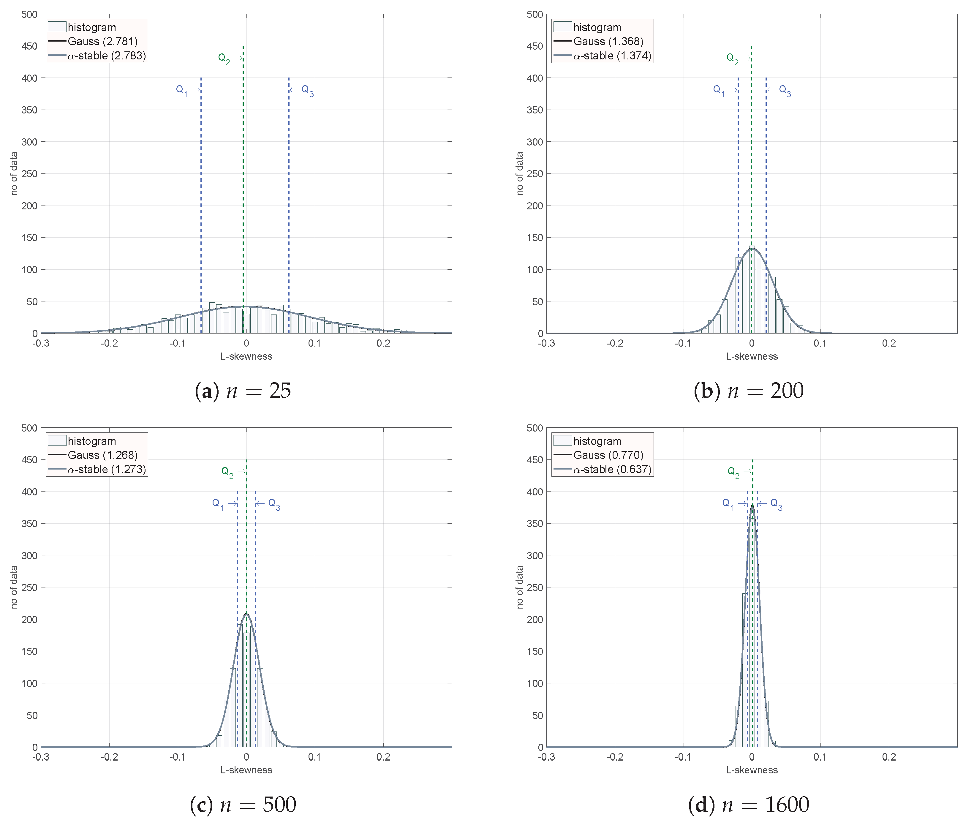
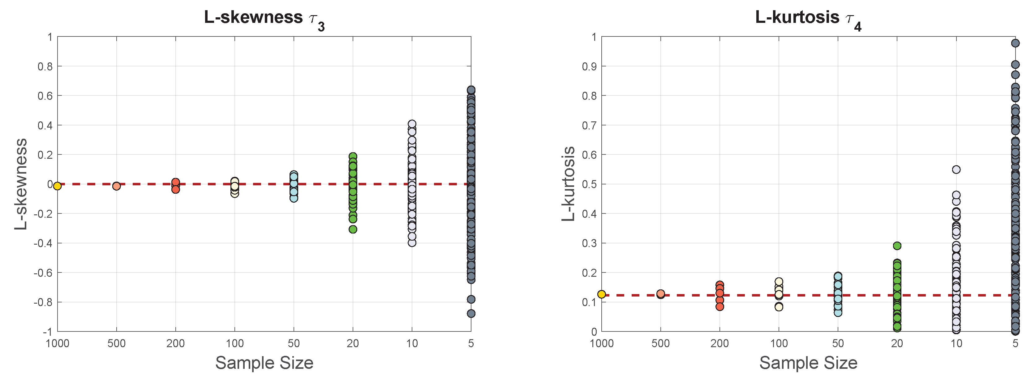
Let us first assess how a sample size affects the LMRD estimation. The experiment is as follows: We take normal distribution $\mathrm{N}\left(0, 1\right)$ and generate $N=1000$ samples. Next, we divide the set into subsets of length $n=\left\{5, 10, 20, 50, 100, 200, 500, N\right\}$. We assess these sample sizes. We obtain $k=\left\{200, 100, 50, 20, 10, 5, 2, 1\right\}$ datasets, respectively. Finally, we calculate the L-skewness and L-kurtosis for each dataset. Figure 2 presents the obtained results. We clearly observe that the smaller the sample size is, the more biased the estimation seems to be.

The results depicted in Figure 2 illustrate how smaller sample sizes lead to increased bias in the estimation of L-moments. This aligns with expectations, as reduced sample sizes limit the robustness of statistical measures. Following this, Figure 3 extends this analysis by showing the histograms of L-skewness for various sample sizes, highlighting how the distribution stabilizes as the sample size increases. These figures underscore the necessity of larger sample sizes in achieving reliable Monte-Carlo estimations, particularly for accurate representations in LMRD.

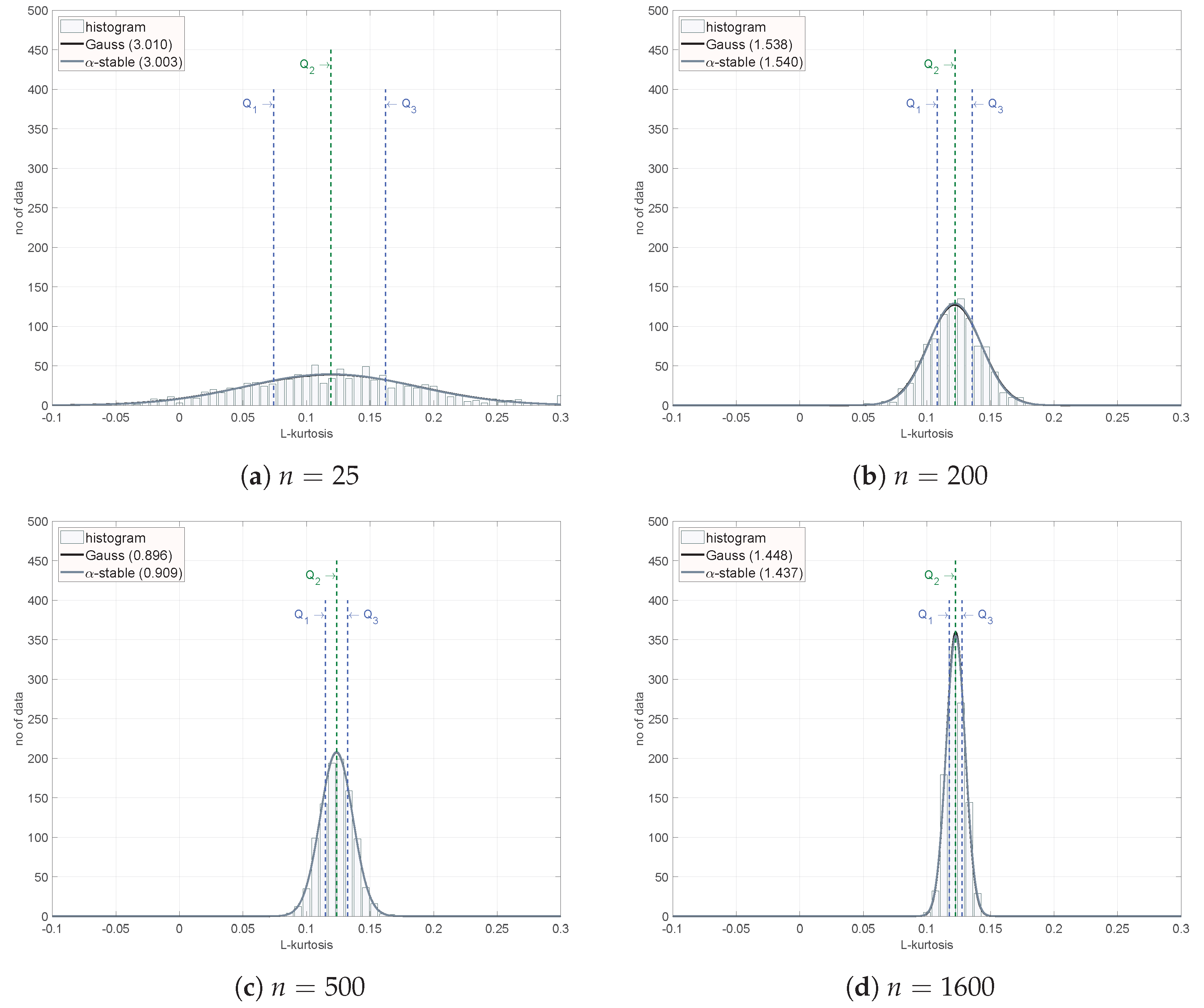
The second experiment aims at investigating how large the sample size should be for good estimation. We repeat the estimation $k=1000$ times for different sizes from $n=25$ till $n=1600$ every 25 samples. For each case, we evaluate histogram and quantiles: Q1, Q2 (median), and Q3. Histograms for ${\tau }_3$ are shown in Figure 3, while Figure 4 shows plots for ${\tau }_4$. It confirms that the sample size might not be too low.

A summary of evaluated estimation metrics, i.e., the quantiles, is shown in Figure 5. An observation of the resulting diagrams leads to the rational decision that the sample size $n=500$ allows for the reliable estimation of L-moments. That number is used in consecutive experiments.

Figure 6 shows LMRD diagrams plotted for normal distribution. Each circle in these plots reflects one population of size $n=500$. We increase the population number and observe properties of LMRD and the estimation. We measure the robust center of scattered points generated for each population as a two-dimensional geometric median (GeoMed) ${\overline{x}}_{\mathrm{med}}$, which is defined as a value of argument $x_0$, to which the sum of all Euclidean distances for $x_i$ is minimized

$${\overline{x}}_{\mathrm{med}}=\underset{x_0\in {\mathbb{R}}^2}{arg\; min}\sum _{i=1}^L{\parallel x_i-x_0\parallel }_2,$$

(14)

where L is the number of points (populations). We evaluate GeoMed with Weiszfeld’s algorithm proposed in [45].

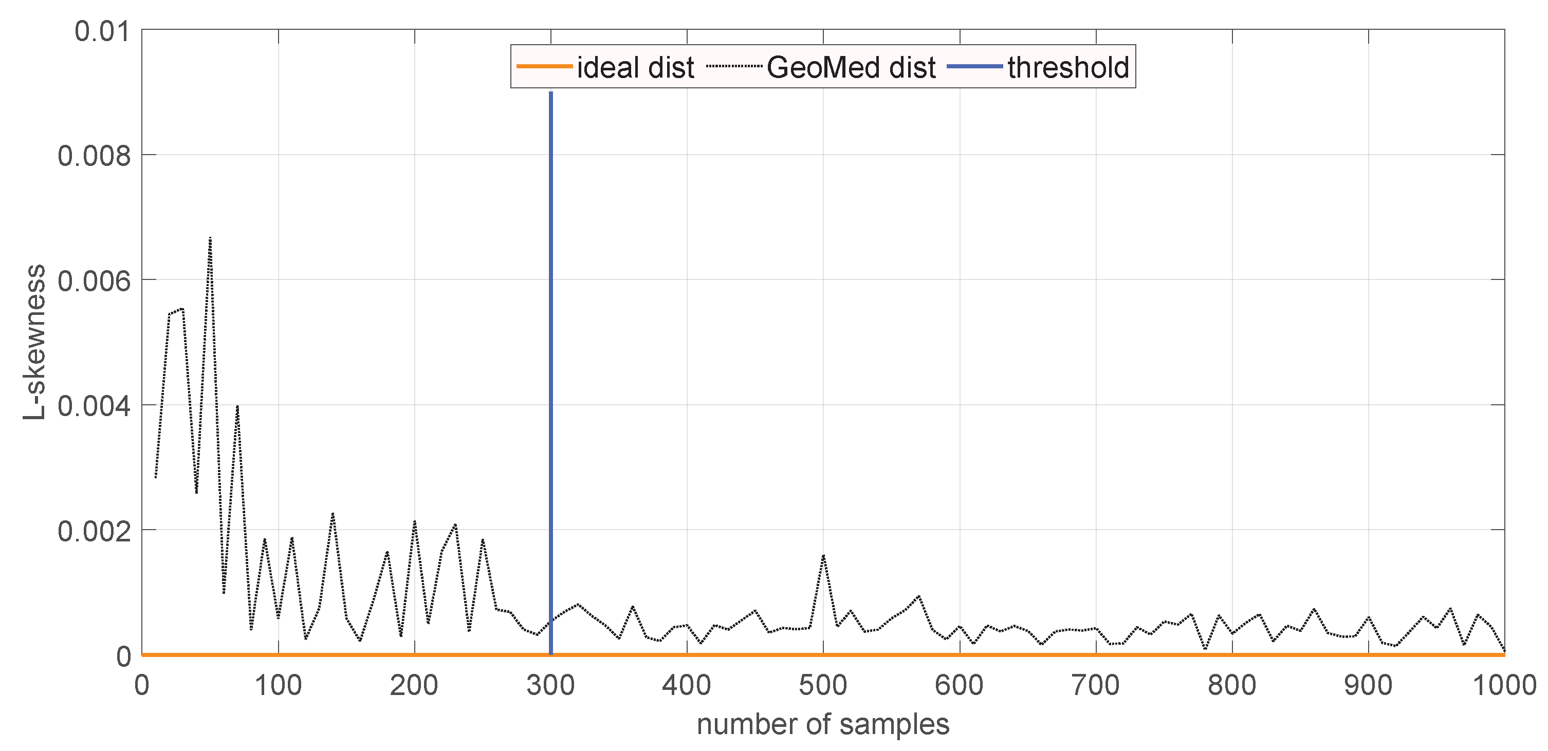
Once the center is known, we measure the distance from the GeoMed point to the point representing ideal normal PDF. This distance measures the estimation efficiency. The more populations we have, the better the estimation that is achieved. The relationship between the population size and the points scatter is shown in Figure 7. Population number $l=300$ enables a reliable PDF fitting.

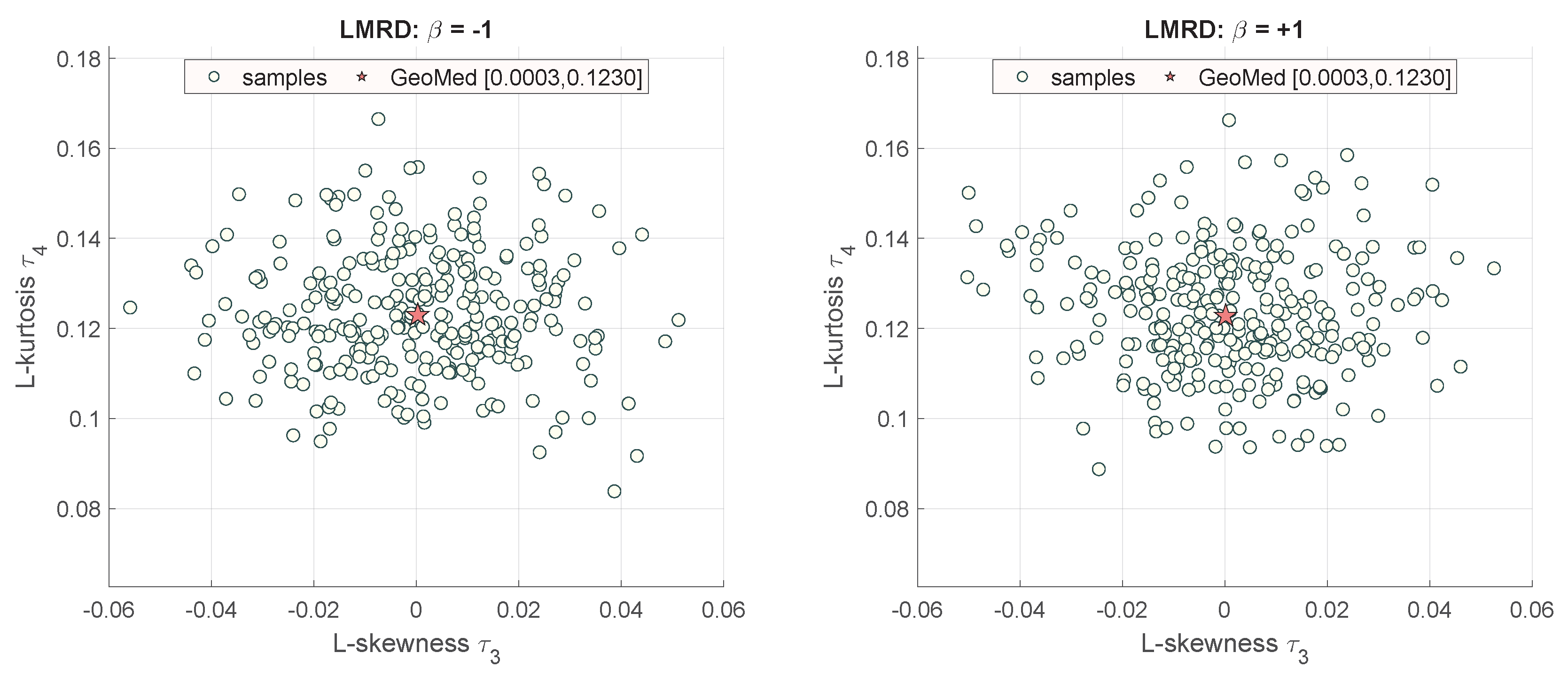
Using the above data, i.e., the sample size $n=500$ and the number of populations $l=300$, we may extend the analysis towards skewed independent distribution described by PDFs ${\mathcal{F}}_{2,\beta ,\delta ,\gamma }^{\mathrm{stab}}\left(x\right)$. Therefore, we set $\delta =0$ and $\gamma =1$, and we draw resulting L-moment ratio diagrams. Figure 8 shows charts for $\beta =-1.0$ and $\beta =+1.0$. Diagrams are exactly the same, and the skewed normal PDF function ${\mathcal{F}}_{2,\beta ,\delta ,\gamma }^{\mathrm{stab}}\left(x\right)$ is always reflected in LMRD(${\tau }_3,{\tau }_4$) diagrams by a single point $\left(0.0, 0.1226\right)$.

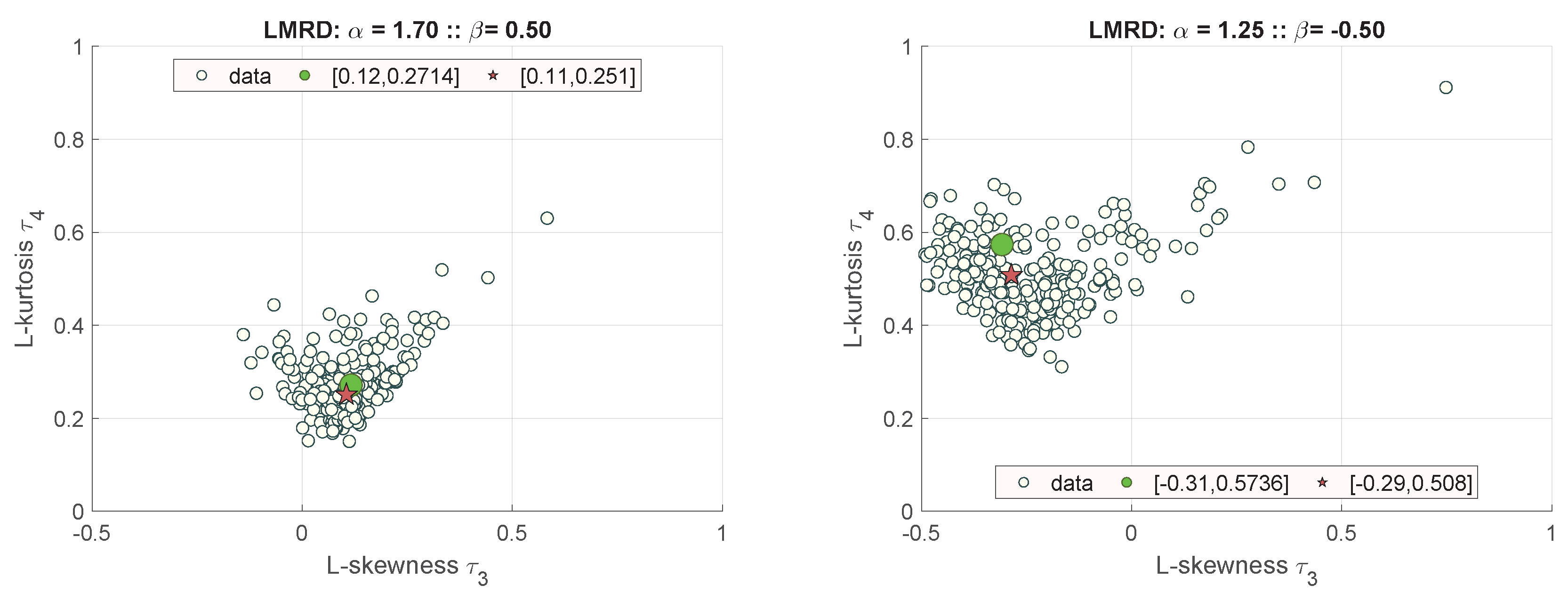
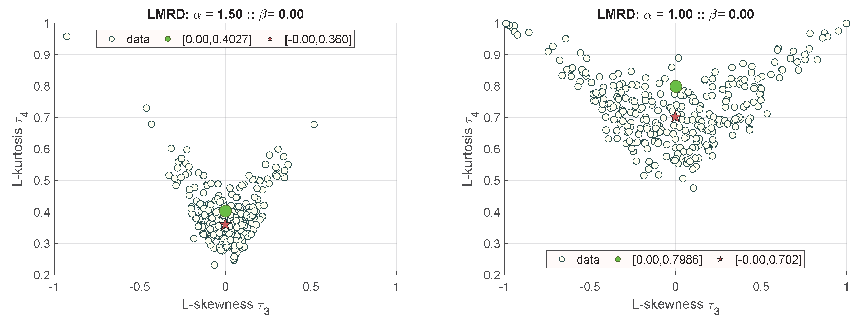
We continue with the general $\alpha$-stable PDF, i.e., for $\alpha \in 〈1, 2〉$. The estimation procedure using LMRD uses above assumptions about the number of samples in each population and the number of populations. Three LMRD(${\tau }_3, {\tau }_4$) diagrams are initially presented. Each of them is prepared for different set of $\alpha$-stable PDF coefficients. The results interpretation problem lies in the lack of theoretical target values. They are called “limiting”. They are estimated using the Monte-Carlo approach with a very large sample size of $n=10,000$ and a high number of populations equal to $l=10,000$. Figure 9 presents estimation for the right-skewed data, while Figure 10 presents the left-skewed parameters. Figure 11 shows symmetrical S$\alpha$S variants. The one with $\alpha =1$ and $\beta =0$ denotes Cauchy PDF. As $\alpha$ diminishes $\alpha \to 1$, the estimation error increases. Estimations tend to decrease values of ${\tau }_3$ and ${\tau }_4$. Therefore, the approach using previously estimated sample and population sizes is highly biased as we recede from independent realization of $\alpha =2.0$.

These results show that sample sizes should not be so low as evaluated for normal distribution. They seriously depend on the stability exponent $\alpha$ value. The estimation performance significantly depends on data tailedness, and it decreases for heavy-tailed data. It is interesting to note that the Cauchy case shown in Figure 11 shows the estimated Monte-Carlo values of L-skewness and L-kurtosis: ${\tau }_3=0.0$ and ${\tau }_4=0.7986$. Generally, it is expected that L-kurtosis for Cauchy distribution should converge to some value. However, this value is a theoretical expectation limit achieved for an infinite sample size.

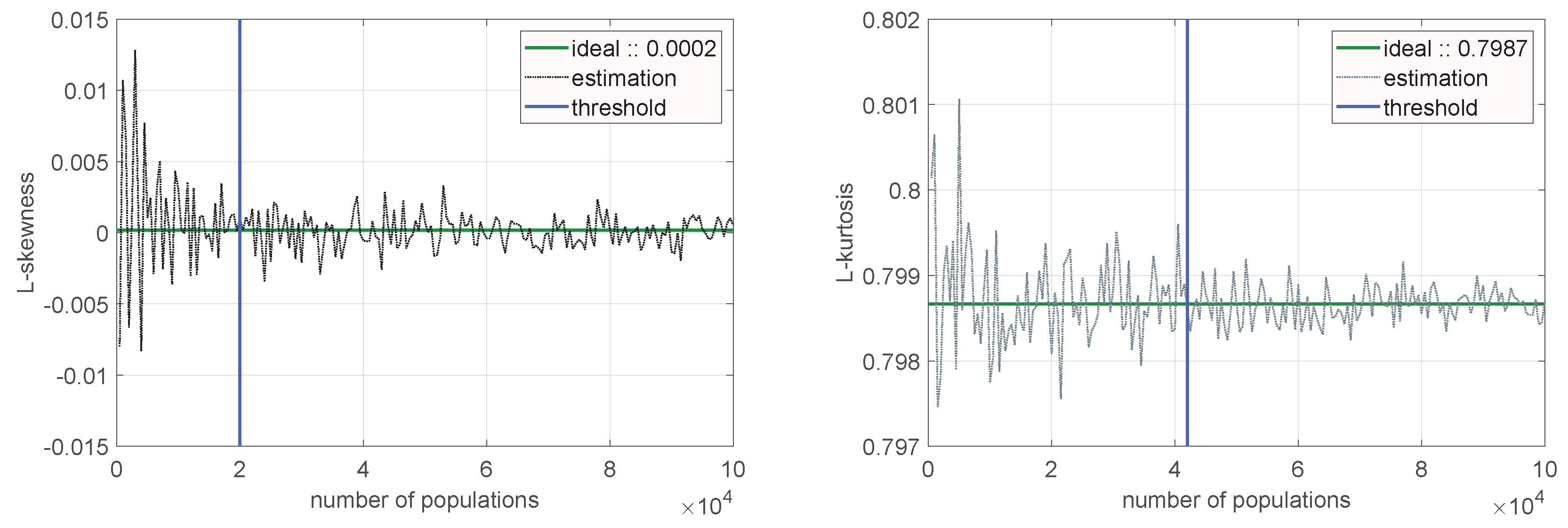
It is interesting to see how the Monte-Carlo L-moments estimation converges for the Cauchy PDF, which is a special case of the $\alpha$-stable distribution (Figure 12). We repeat consecutive estimations, assuming sample size n = 10,000 and changing the number of populations $l=500,\dots ,100,000$. The target values of L-moments are evaluated using robust location estimator with logistic M-function as in [46]. Concluding, we might use the following estimated L-moments for Cauchy distribution: ${\tau }_3^{\left(\mathrm{MC}\right)}=0.0$ and ${\tau }_4^{\left(\mathrm{MC}\right)}=0.799$. L-kurtosis differs significantly from TL-kurtosis given by [47], i.e., ${\tau }_4^{\left(\mathrm{l}\right)}=0.343$.

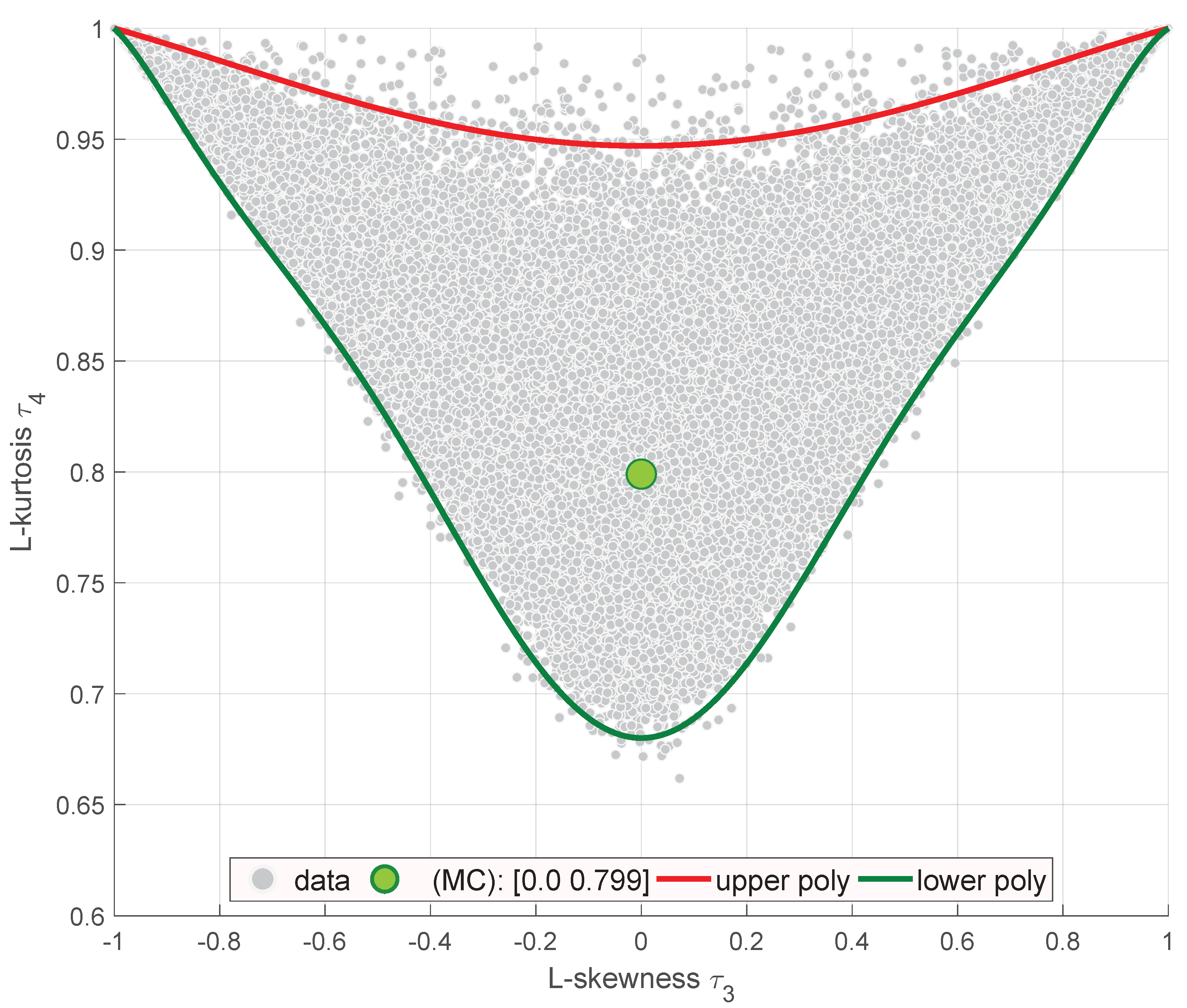
The respective plot for the highest population number l = 100,000 is given in Figure 13. Obtained points can be approximated by upper and lower bounds. The estimation is given by the analogous Equation (13), with its coefficients shown in

Table 3. Polynomial coefficients for Cauchy distribution.

	${\mathit{a}}_0$	${\mathit{a}}_1$	${\mathit{a}}_2$	${\mathit{a}}_3$	${\mathit{a}}_4$	${\mathit{a}}_5$	${\mathit{a}}_6$	${\mathit{a}}_7$	${\mathit{a}}_8$
lower	0.68	0	0.9078	−0.0305	−1.6336	0.078	1.7292	−0.0476	−0.6834
upper	0.947	0	0.0725	0	−0.0195

.

Obtained boundary curves are highly similar to the skewness-kurtosis chart for the truncated Cauchy distribution [48]. Obtained results are somehow disappointing, as for proper and converging estimation we require extremely large number of observations, both in sample size and the population number. We also notice that the heavier the tail is, the more points are required to evaluate the proper GeoMed Monte-Carlo estimator of L-moments. This is hardly achievable in real life datasets.

Nonetheless, the same experiment is repeated for $\alpha$-stable distribution. At first, we generate large number l = 10,000 of populations of size $n=2000$. We use the $\alpha$-stable random numbers generator and generate data for ${\mathcal{F}}_{\alpha ,\beta ,0,1}^{\mathrm{stab}}\left(x\right)$. The stability factor changes $\alpha =\left\{1.0,\dots ,2.0\right\}$ with a decrement $\Delta \alpha =0.1$ and $\beta =\left\{-1.0,\dots ,+1.0\right\}$ with a decrement $\Delta \beta =0.25$. For each point, we find a GeoMed center.

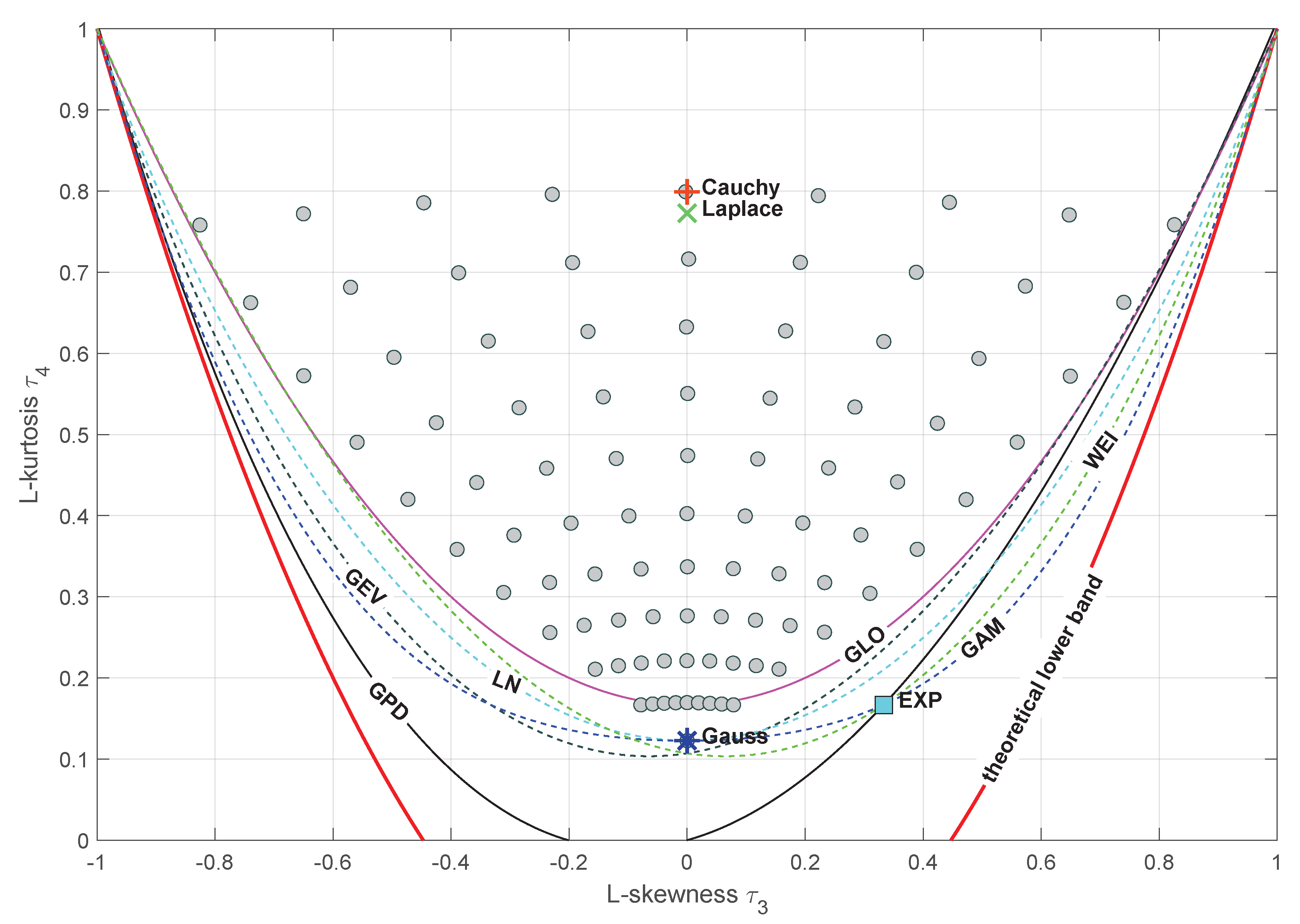
Figure 14 presents clear L-moment ratio diagram with such evaluated GeoMed centers in the background of characteristic points for other known distributions as given in Table 1 and Table 2. We see exact cover for two special cases, i.e., Gaussian and Cauchy functions, previously evaluated.

These points arrange themselves into specific shapes, which are symmetrical in the vertical axis ${\tau }_3=0$. Figure 15a connects these points with straight lines, while Figure 15b interpolates them with polynomial functions Equation (13). Coefficients of polynomials for $\alpha$ are given in

Table 4. Monte-Carlo polynomials for varying stability index $\alpha$.

$\mathit{\alpha }$	1.0	1.1	1.2	1.3	1.4	1.5	1.6	1.7	1.8	1.9
$a_0$	0.799	0.716	0.632	0.550	0.474	0.403	0.337	0.277	0.221	0.170
$a_1$	−0.074	−0.114	−0.167	−0.211	−0.280	−0.325	−0.378	−0.410	−0.514	−0.571
$a_2$	0.020	0.030	0.057	0.066	0.170	0.221	0.458	0.559	2.981	19.729

and for $\beta$ in

Table 5. Monte-Carlo polynomials for varying skewness factor $\beta$.

$\mathit{\beta }$	−1.0	−0.75	−0.5	−0.25	0	0.25	0.5	0.75	1.0
$a_0$	0.123	0.124	0.123	0.125	-	0.125	0.123	0.124	0.123
$a_1$	−0.546	−0.707	−1.079	−2.093	-	2.093	1.079	0.707	0.546
$a_2$	0.046	0.001	1.876	9.885	-	9.701	1.893	0.598	0.045
$a_3$	−0.273	0.232	2.148	26.305	-	−26.305	−2.148	−0.232	0.273

.

Polynomials that reflect variations in L-skewness are symmetrical and have an order 2. The polynomials reflecting variations of stability exponent $\alpha$ are of order 3, and the ones with the same absolute value of $\left|\beta \right|$ are symmetrical against each other around axis OY. Monte-Carlo estimation allows us to estimate the LMRD estimations for additional special cases, i.e., Holtsmark and Landau. Moments of Landau PDF, such as mean or variance, are undefined, while Holtsmark has mean, its variance is infinite, and higher moments undefined.

Table 6. Estimated ${\tau }_3^{\left(\mathrm{MC}\right)}$ and ${\tau }_4^{\left(\mathrm{MC}\right)}$ of $\alpha$-stable function special cases.

	${\mathit{\tau }}_3^{\left(\mathbf{MC}\right)}$	${\mathit{\tau }}_4^{\left(\mathbf{MC}\right)}$
Landau	0.8259	0.7586
Holtsmark	0.0	0.4025

shows estimated LMRD(${\tau }_3,{\tau }_4$) points.

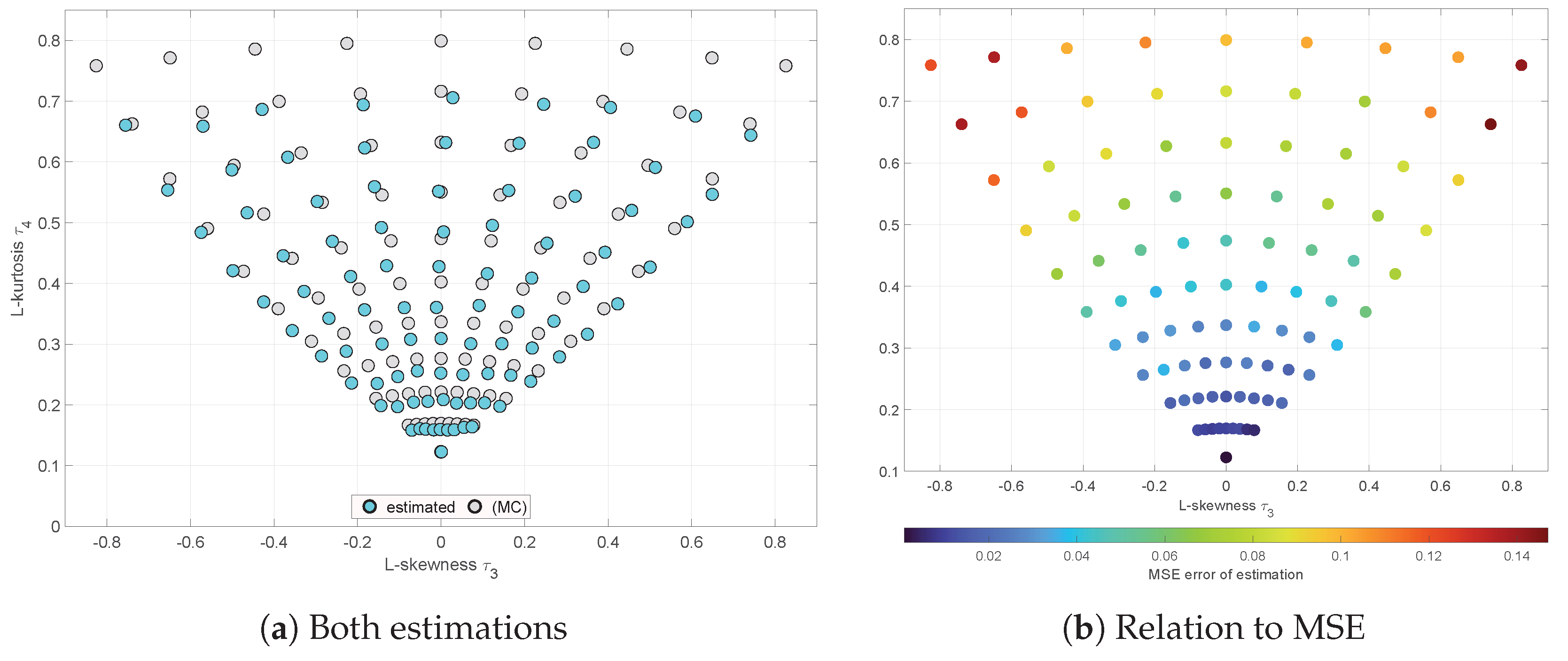
The estimation error rises as tails get heavier, i.e., as stability exponent diminishes. Figure 16a compares Monte-Carlo simulations (denoted [MC]) with sample size $n=500$ and number of populations $l=300$. Figure 16b relates $\left[{\tau }_3^{\left(\mathrm{MC}\right)},{\tau }_4^{\left(\mathrm{MC}\right)}\right]$ to the estimation mean square error (MSE).

Error performance related to the stability index $\alpha$ is shown in Figure 17. The effect of estimation error deterioration and the need for higher sample sizes is obvious. We observe close to linear trend. The trend slope increases with the increasing absolute value of skewness $\beta$. This feature is highly disappointing, because it seriously limits practical implementations, demanding extremely high observation numbers to get reliable estimation. Moreover, we have to keep in mind that similarly to the Cauchy case real theoretical values might even be different, as the values converge with an increased number of samples, and the infinity cannot be captured in simulations.

4. Conclusions

The paper analyzes properties of L-moments for $\alpha$-stable distribution. Despite the fact of infinite or undefined higher moments of stable functions, it is shown that there might exist limiting estimations, called Monte-Carlo estimates, for L-skewness ${\tau }_3^{\left(\mathrm{MC}\right)}$ and L-kurtosis ${\tau }_3^{\left(\mathrm{MC}\right)}$.

The main contribution of the paper is the evaluation of the polynomial curves of $\alpha$-stable distribution for LMRD(${\tau }_3,{\tau }_4$) diagrams. Their evaluation is accompanied by an extensive analysis of limiting Gauss and Cauchy cases. We clearly see that significantly high sample sizes are required to get closer to theoretical limiting values.

In this sense, the paper is novel, as respective approaches are not found in the literature.

Future research could explore the use of trimmed L-moments (TL-moments) to further enhance the robustness of estimations in heavy-tailed data scenarios. Exploring alternative ordered moments, such as LH-, LL-, LQ-, or PL-moments, may also provide avenues to reduce the required sample sizes while maintaining estimation accuracy, making this approach more accessible for real-world applications with limited data.

References

1. Wainer, H. Robust Statistics: A Survey and Some Prescriptions. J. Educ. Stat. 1976, 1, 285–312. [Google Scholar] [CrossRef]
2. Nair, J.; Wierman, A.; Zwart, B. The Fundamentals of Heavy Tails: Properties, Emergence, and Estimation; Cambridge Series in Statistical and Probabilistic Mathematics; Cambridge University Press: Cambridge, UK, 2022. [Google Scholar]
3. Foss, S.; Korshunov, D.; Zachary, S. Heavy-Tailed and Long-Tailed Distributions. In An Introduction to Heavy-Tailed and Subexponential Distributions; Springer: New York, NY, USA, 2013; pp. 7–42. [Google Scholar]
4. Domański, P.D. Control quality assessment using fractal persistence measures. ISA Trans. 2019, 90, 226–234. [Google Scholar] [CrossRef]
5. Mandelbrot, B.B.; Hudson, R.L. The Misbehavior of Markets: A Fractal View of Financial Turbulence; Basic Books: New York, NY, USA, 2004. [Google Scholar]
6. Taleb, N.N. Statistical Consequences of Fat Tails: Real World Preasymptotics, Epistemology, and Applications. arXiv 2022, arXiv:2001.10488v3. [Google Scholar] [CrossRef]
7. Hurst, H.; Black, R.; Simaika, Y. Long-Term Storage: An Experimental Study; Constable: London, UK, 1965. [Google Scholar]
8. Sheng, H.; Chen, Y.; Qiu, T. Fractional Processes and Fractional-Order Signal Processing; Springer: London, UK, 2012. [Google Scholar]
9. Domański, P.D. Back to Statistics. Tail-Aware Control Performance Assessment; CRC Press; Taylor & Francis Group: Boca Raton, FL, USA, 2025. [Google Scholar]
10. Bobee, B.; Perreault, L.; Ashkar, F. Two kinds of moment ratio diagrams and their applications in hydrology. Stoch. Hydrol. Hydraul. 1993, 7, 41–65. [Google Scholar] [CrossRef]
11. Hosking, J.; Wallis, J.R. Regional Frequency Analysis: An Approach Based on L-Moments; Cambridge University Press: Cambridge, UK, 1997. [Google Scholar] [CrossRef]
12. Domański, P.D.; Dziuba, K.; Góra, R. PID Control Assessment Using L-Moment Ratio Diagrams. Appl. Sci. 2024, 14, 3331. [Google Scholar] [CrossRef]
13. Hosking, J. L-Moments: Analysis and Estimation of Distributions Using Linear Combinations of Order Statistics. J. R. Stat. Soc. Ser. B (Methodol.) 1990, 52, 105–124. [Google Scholar] [CrossRef]
14. Hosking, J. Moments or L Moments? An Example Comparing Two Measures of Distributional Shape. Am. Stat. 1992, 46, 186–189. [Google Scholar] [CrossRef]
15. Hosking, J. Some theory and practical uses of trimmed L-moments. J. Stat. Plan. Inference 2007, 137, 3024–3039. [Google Scholar] [CrossRef]
16. Kjeldsen, T.; Ahn, H.; Prosdocimi, I. On the use of a four-parameter kappa distribution in regional frequency analysis. Hydrol. Sci. J. 2017, 62, 1354–1363. [Google Scholar] [CrossRef]
17. Hosking, J. L-Moments and Their Applications in the Analysis of Financial Data; Technical Report RC 21466 (96889); IBM Research Division: Yorktown Heights, NY, USA, 1999. [Google Scholar]
18. Domański, P.D.; Jankowski, R.; Dziuba, K.; Góra, R. Assessing Control Sustainability Using L-Moment Ratio Diagrams. Electronics 2023, 12, 2377. [Google Scholar] [CrossRef]
19. Khan, M.; Hussain, Z.; Sher, S.; Amjad, M.; Baig, F.; Ahmad, I.; Ullah, H. A comparative analysis of L-moments, maximum likelihood, and maximum product of spacing methods for the four-parameter kappa distribution in extreme value analysis. Sci. Rep. 2025, 15, 164. [Google Scholar] [CrossRef]
20. Nolan, J.P. Stable Regression. In Univariate Stable Distributions: Models for Heavy Tailed Data; Springer International Publishing: Cham, Swizterland, 2020; pp. 223–238. [Google Scholar] [CrossRef]
21. Ross, S. (Ed.) Introduction to Probability Models, 11th ed.; Academic Press: Boston, MA, USA, 2014. [Google Scholar] [CrossRef]
22. Royuela-del-Val, J.; Simmross-Wattenberg, F.; Alberola-Lopez, C. libstable: Fast, parallel, and high-precision computation of α-stable distributions in R, C/C++, and MATLAB. J. Stat. Softw. Artic. 2017, 78, 1–25. [Google Scholar] [CrossRef]
23. Koutrouvelis, I.A. Regression-Type Estimation of the Parameters of Stable Laws. J. Am. Stat. Assoc. 1980, 75, 918–928. [Google Scholar] [CrossRef]
24. McCulloch, J.H. Simple consistent estimators of stable distribution parameters. Commun. Stat.-Simul. Comput. 1986, 15, 1109–1136. [Google Scholar] [CrossRef]
25. Kuruoglu, E. Density parameter estimation of skewed alpha-stable distributions. IEEE Trans. Signal Process. 2001, 49, 2192–2201. [Google Scholar] [CrossRef]
26. Borak, S.; Misiorek, A.; Weron, R. Models for heavy-tailed asset returns. In Statistical Tools for Finance and Insurance, 2nd ed.; Cizek, P., Härdle, W., Weron, R., Eds.; Springer: Berlin/Heidelberg, Germany, 2011; pp. 21–56. [Google Scholar] [CrossRef]
27. Bodnar, T.; Otryakhin, D.; Thorsén, E. Estimation of the multivariate symmetric stable distribution using the method of moments. Commun. Stat.-Theory Methods 2025, 54, 5039–5056. [Google Scholar] [CrossRef]
28. Duda, J. Adaptive stable distribution and Hurst exponent by method of moments moving estimator for nonstationary time series. arXiv 2025, arXiv:2506.05354v1. [Google Scholar] [CrossRef]
29. Hajjaji, O.; Manou-Abi, S.M.; Slaoui, Y. Parameter estimation for stable distributions and their mixture. J. Appl. Stat. 2025, 52, 1594–1627. [Google Scholar] [CrossRef]
30. Pączek, K.; Jelito, D.; Pitera, M.; Wyłomańska, A. Estimation of stability index for symmetric α-stable distribution using quantile conditional variance ratios. TEST 2024, 33, 297–334. [Google Scholar] [CrossRef]
31. Skowronek, K.; Arendarczyk, M.; Panorska, A.; Kozubowski, T.; Wyłomańska, A. Testing and estimation of the index of stability of univariate and bivariate symmetric α-stable distributions via modified Greenwood statistic. J. Comput. Appl. Math. 2025, 467, 116587. [Google Scholar] [CrossRef]
32. Domański, P.D. Statistical measures for proportional–integral–derivative control quality: Simulations and industrial data. Proc. Inst. Mech. Eng. Part I J. Syst. Control Eng. 2018, 232, 428–441. [Google Scholar] [CrossRef]
33. Brown, L.D.; Gene Hwang, J.T. How to Approximate a Histogram by a Normal Density. Am. Stat. 1993, 47, 251–255. [Google Scholar] [CrossRef]
34. Hazelton, M.L. Methods of Moments Estimation. In International Encyclopedia of Statistical Science; Lovric, M., Ed.; Springer: Berlin/Heidelberg, Germany, 2011; pp. 816–817. [Google Scholar] [CrossRef]
35. Simková, T. Statistical inference based on L-moments. Stat. Stat. Econ. J. 2017, 97, 44–58. [Google Scholar]
36. Peel, M.; Wang, Q.; Mcmahon, T. The utility L-moment ratio diagrams for selecting a regional probability distribution. Hydrol. Sci. J. 2001, 46, 147–155. [Google Scholar] [CrossRef]
37. Giełczewski, M.; Piniewski, M.; Domański, P. Mixed statistical and data mining analysis of river flow and catchment properties at regional scale. Stoch. Environ. Res. Risk Assess. 2022, 36, 2861–2882. [Google Scholar] [CrossRef]
38. Neykov, N.M.; Neytchev, P.N.; Van Gelder, P.H.A.J.M.; Todorov, V.K. Robust detection of discordant sites in regional frequency analysis. Water Resour. Res. 2007, 43, W06417. [Google Scholar] [CrossRef]
39. Craig, C. A New Exposition and Chart for the Pearson System of Frequency Curves. Ann. Math. Stat. 1936, 7, 16–28. [Google Scholar] [CrossRef]
40. Vargo, E.; Pasupathy, R.; Leemis, L. Moment-Ratio Diagrams for Univariate Distributions. J. Qual. Technol. 2010, 42, 276–286. [Google Scholar] [CrossRef]
41. Cox, D.; Oakes, D. Analysis of Survival Data; Chapman and Hall: London, UK, 1984. [Google Scholar] [CrossRef]
42. Haddad, K. Selection of the best fit probability distributions for temperature data and the use of L-moment ratio diagram method: A case study for NSW in Australia. Theor. Appl. Climatol. 2021, 143, 1261–1284. [Google Scholar] [CrossRef]
43. Delicado, P.; Goria, M. A small sample comparison of maximum likelihood, moments and L-moments methods for the asymmetric exponential power distribution. Comput. Stat. Data Anal. 2008, 52, 1661–1673. [Google Scholar] [CrossRef]
44. Kirby, W. Algebraic boundedness of sample statistics. Water Resour. Res. 1974, 10, 220–222. [Google Scholar] [CrossRef]
45. Weiszfeld, E.; Plastria, F. On the point for which the sum of the distances to n given points is minimum. Ann. Oper. Res. 2009, 167, 37–41. [Google Scholar] [CrossRef]
46. Verboven, S.; Hubert, M. LIBRA: A Matlab library for robust analysis. Chemom. Intell. Lab. Syst. 2005, 75, 127–136. [Google Scholar] [CrossRef]
47. Elamir, E.; Seheult, A. Trimmed L-moments. Comput. Stat. Data Anal. 2003, 43, 299–314. [Google Scholar] [CrossRef]
48. Nadarajah, S. Making the Cauchy work. Braz. J. Probab. Stat. 2011, 25, 99–120. [Google Scholar] [CrossRef]
Figure 1. LMRD( τ 3 ,   τ 4 ) diagram with theoretical functions.
Fractalfract 09 00711 g001
Figure 2. Sample size impact on L-moments estimation; dashed red line depicts ideal values.
Fractalfract 09 00711 g002
Figure 3. Histograms of L-skewness estimation related to sample size n. Gauss line is hidden behind α -stable.
Fractalfract 09 00711 g003
Figure 4. Histograms of L-kurtosis estimation related to sample size n. Gauss line is hidden behind α -stable.
Fractalfract 09 00711 g004
Figure 5. Convergence of quantiles related to the sample size.
Fractalfract 09 00711 g005
Figure 6. LMRD( τ 3 , τ 4 ): green circle shows ideal point, black cross GeoMed.
Fractalfract 09 00711 g006
Figure 7. Distance from ideal point related to the number of experiments.
Fractalfract 09 00711 g007
Figure 8. LMRD( τ 3 , τ 4 ) for β = 1.0 and β = + 1.0 .
Fractalfract 09 00711 g008
Figure 9. Right-skewed LMRD( τ 3 , τ 4 ): green circle is limiting value, red star estimated.
Fractalfract 09 00711 g009
Figure 10. Left-skewed LMRD( τ 3 , τ 4 ): green circle is limiting value, red star estimated.
Fractalfract 09 00711 g010
Figure 11. S α S data LMRD( τ 3 , τ 4 ): green circle is limiting value, red star estimated.
Fractalfract 09 00711 g011
Figure 12. Monte Carlo L-moments estimations for Cauchy distribution.
Fractalfract 09 00711 g012
Figure 13. Convergence of Monte-Carlo L-moments estimations for Cauchy distribution; (MC) denotes Monte Carlo estimation τ 3 ( MC ) ;   τ 4 ( MC ) .
Fractalfract 09 00711 g013
Figure 14. LMRD with Monte-Carlo GeoMed estimations.
Fractalfract 09 00711 g014
Figure 15. LMRD( τ 3 , τ 4 ) maps for α -stable distribution.
Fractalfract 09 00711 g015
Figure 16. LMRD( τ 3 , τ 4 ) maps with Monte-Carlo and small size estimations.
Fractalfract 09 00711 g016
Figure 17. LMRD with Monte-Carlo GeoMed estimations for α -stable PDF.
Fractalfract 09 00711 g017