Article

Iterative Investigation of the Nonlinear Fractional Cahn–Allen and Fractional Clannish Random Walker’s Parabolic Equations by Using the Hybrid Decomposition Method

1
State Key Laboratory of Intelligent Geotechnics and Tunnelling, Shenzhen University, Shenzhen 518060, China
2
Department of Mathematics and Statistics, College of Science, Imam Mohammad Ibn Saud Islamic University (IMSIU), Riyadh 11564, Saudi Arabia
3
Department of Mathematics, COMSATS University Islamabad, Lahore Campus, Lahore 54000, Pakistan
4
Mathematics Department, Faculty of Science, Taibah University, Al-Madinah Al-Munawarah 41411, Saudi Arabia
5
Basic Sciences Research Center (BSRC), Deanship of Scientific Research, Imam Mohammad Ibn Saud Islamic University (IMSIU), Riyadh 13318, Saudi Arabia
*
Author to whom correspondence should be addressed.
Fractal Fract. 2025, 9(10), 656; https://doi.org/10.3390/fractalfract9100656
Submission received: 2 September 2025 / Revised: 5 October 2025 / Accepted: 8 October 2025 / Published: 11 October 2025
(This article belongs to the Special Issue Applications of Fractional Calculus in Modern Mathematical Modeling)

Abstract

In this work, we numerically investigate the fractional clannish random walker’s parabolic equations (FCRWPEs) and the nonlinear fractional Cahn–Allen (NFCA) equation using the Hybrid Decomposition Method (HDM). The analysis uses the Atangana–Baleanu fractional derivative (ABFD) in the Caputo sense, which has a nonsingular and nonlocal Mittag–Leffler kernel (MLk) and provides a more accurate depiction of memory and heredity effects, to examine the dynamic behavior of the models. Using nonlinear analysis, the uniqueness of the suggested models is investigated, and distinct wave profiles are created for various fractional orders. The accuracy and effectiveness of the suggested approach are validated by a number of example cases, which also support the approximate solutions of the nonlinear FCRWPEs. This work provides significant insights into the modeling of anomalous diffusion and complex dynamic processes in fields such as phase transitions, biological transport, and population dynamics. The inclusion of the ABFD enhances the model’s ability to capture nonlocal effects and long-range temporal correlations, making it a powerful tool for simulating real-world systems where classical derivatives may be inadequate.

1. Introduction

In physics, engineering, biology, and other applied sciences, nonlinear partial differential equations (NLPDEs) are essential for simulating a variety of complex phenomena [1,2,3,4,5,6]. In contrast to their linear counterparts, NPDEs capture key elements that are inherent to many real-world systems, including shock waves, turbulence, pattern development, wave interactions, and chaos [7,8,9]. Fluid dynamics, quantum mechanics, nonlinear optics, plasma physics, and biological processes are just a few of the fields in which they naturally occur [10,11,12]. Therefore, it is essential to fully understand NPDEs in order to advance theoretical knowledge and enhance the predictive power of mathematical models utilized in technical and scientific applications [13,14,15]. Then finding solutions of various NPDEs is a hot topic so, many analytical techniques are developed in nonlinear theory for instance [16,17,18]: Nonlinearities [1], transformations technique [2], modified sub-equation technique [11], Sine–Gordon expansion method [12], Laplace homotopy scheme [13], generalized exponential function method [14], auxiliary equation method [15], expansion scheme [16], Instability analysis technique [17], appropriate transformation method [18], etc.
The ability of fractional differential equations (FDEs) to more accurately model memory-dependent and hereditary phenomena than traditional integer-order differential equations has drawn a lot of attention in recent years. In contrast to conventional models, FDEs use fractional derivatives and nonlocal operators to capture complicated dynamical phenomena present in a variety of real-world systems, including fluid dynamics, anomalous diffusion, biological systems, viscoelastic materials, and signal processing. Chita et al. studied a new approach for solving FDEs via a multistage telescoping decomposition technique [19]. Chakraverty et al. examined the computation and modeling for fractional order systems [20]. Amilo et al. studied the Caputo and variable-order fractional derivative algorithms across various applications [21]. Atangana et al. studied examples and applications of FDEs via fractional differential and integral operators [22], Boukedroun et al. investigated the solutions of nonlinear fractional FDEs via numerical techniques [23]. The mathematical modeling framework has been enhanced by the addition of fractional-order derivatives, such as the Riemann–Liouville, Caputo, and more recently, ABFD [24,25]. These derivatives offer strong tools for characterizing systems with spatial or temporal memory effects [26,27]. These operators provide more modeling flexibility, enabling an improved representation of physical processes in scenarios where traditional methods might not be sufficient [28,29]. As a result, research and numerical analysis of FDEs has grown significantly in applied mathematics and engineering [30,31]. Specifically, the Caputo derivative represents systems with memory and hereditary properties, where the present state depends on the entire history of the process, making it suitable for modeling viscoelastic and diffusion phenomena. The ABFD, on the other hand, introduces a nonsingular MLk, which captures nonlocal and non-singular memory effects more realistically. It provides a smoother transition between past and present states, describing processes with fading memory and long-term temporal correlations more accurately than traditional fractional operators.
HDM is the combination of Adomian and Laplace Adomian techniques. Classical integer-order derivatives often fail to capture the memory, hereditary, and anomalous diffusion effects observed in many physical, biological, and chemical processes. The NFCA equation describes phase transition phenomena, where long-range temporal correlations play a crucial role. Similarly, the FCRWPEs model population dynamics and transport processes, which inherently exhibit nonlocality and memory. Fractional calculus provides a more realistic framework because the fractional derivative accounts for history-dependent behavior, making it particularly suitable for these models. Our use of the ABFD in the Caputo sense is characterized by a nonsingular MLk. This formulation includes long-range correlations that are not present in conventional calculus and depicts memory effects that gradually lose their impact [32,33]. Physically speaking, this implies that the system’s future state is dependent on both its current state and its complete historical evolution [34,35]. This is essential for precisely modeling anomalous diffusion, visco elasticity, phase separation, and intricate biological transport mechanisms [36,37].

Advantages and Disadvantages of the Hybrid Decomposition Method (HDM)

  • Advantages:
    -
    Handles fractional operators naturally via the Laplace transform (clean initial condition embedding) and treats nonlinearity by decomposition, yielding rapidly convergent series with few terms.
    -
    Achieves low truncation/residual errors and robust performance across fractional orders β ; recovers the classical model smoothly as β 1 .
    -
    Moderate computational cost; analytic-like series enable easy parameter sweeps and clear physical interpretation.
    -
    Avoids the full complexity of polynomial generation in purely ADM-type schemes; hybridization improves stability/accuracy.
  • Disadvantages:
    -
    Convergence is problem- and domain-dependent; accuracy may deteriorate for large time/spatial ranges or strong nonlinearities unless more terms are retained.
    -
    Requires Laplace inversion and smooth data; complex boundary conditions, external forcing, or irregular geometries can complicate the pipeline.
    -
    Truncation-error control is empirical unless a contraction proof is available; residual checks are needed to certify accuracy.
    -
    Extension to higher dimensions or discontinuous solutions (e.g., shocks) can reduce efficiency and may require additional stabilization.
In this work, we discuss the uniqueness and numerical study of the FCRWP equation which is as follows [38]:
β u t β u x + 2 u u x + 2 u x 2 = 0 t > 0 , β > 0 , u ( x , t ) = g ( x ) .
We would like to clarify that when β = 1 , the fractional derivative reduces to the classical first-order time derivative, and Equation (1) indeed recovers the standard non-fractional version of the FCRWPE. This confirms that our model is a natural generalization of the classical equation to the fractional framework. For β > 1 or other positive integer values, the equation involves higher-order time derivatives, but our focus in this work is primarily on 0 < β 1 , where the ABFD provides a more accurate description of memory and nonlocal effects. This fractional generalization allows us to capture anomalous diffusion and hereditary properties, which cannot be represented by the standard integer-order case and we will also discuss the uniqueness and numerical study of the NFCA-equation which is described in [39,40,41]. A detailed comparison between our previous studies can be seen in Table 1.
β u t β + u 3 2 u x 2 u = 0 t > 0 , β > 0 , u ( x , t ) = g ( x ) .
The material of this manuscript is arranged as follows: In Section 2, we will give preliminaries containing basic definitions and results helpful in our work. In Section 3, we will give the solution procedure for the FCRWP equation. Section 4 contains the solution procedure for NFCA-equation and Section 5 presents the discussion and applications of the FCRWP equation and NFCA-equation with various three-dimensional, two-dimensional and contour graphs for our some of our new solutions. In Section 6, we will give Error analysis and residual verification. Section 7 contains the comparative numerical discussion to highlight the applicability of the proposed HDM-Laplace scheme. Furthermore, in Section 8 physical interpretation of the fractional order β is given. In Section 9, we provide the results and observations, and finally, in Section 10, we will present the concluding remarks.

2. Preliminaries

In this section, we introduce some basic definitions and results helpful in our work.

2.1. Definition

For a function u W ( 0 , T ) , the fractional ABC is defined as follows [3]:
D 0 + β A B C u ( θ ) = N β 1 β 0 θ E β β 1 β θ v β u v d v ,
where N ( β ) stands for normalization function along with N ( 1 ) = N ( 0 ) = 1 and E β = α = 0 η α Γ β α + 1 shows MLk function.

2.2. Definition

For a function u N ( 0 , T ) , the fractional ABC is defined as follows [3]:
I 0 + β A B C u ( θ ) = 1 β N β u ( θ ) + β N β Γ ( β ) 0 θ θ v β 1 u v d v .

2.3. Definition

The Laplace transform (LT) for a function ψ ( θ ) having the property of piece-wise continuity is defined as follows [3]:
£ ψ θ = 0 e s θ ψ θ d θ f o r θ ϵ [ 0 , ) ,
where s belong to complex set.

2.4. Definition

The LT of ABC for a function ψ ( θ ) is given as [3]
£ D 0 + β A B C ψ ( θ ) = N β s β 1 1 β + β s β £ ψ θ s β 1 ψ 0 .
To solve the stated model, we assume the required solution in the form below:
ψ ( x , θ ) = k = 0 ψ k ( x , θ ) .
and nonlinearity is expressed as
N ψ ( x , θ ) = n = 0 A n ( x , θ ) ,
where A n stands for Adomian polynomials and are specified by
A n ( x , θ ) = 1 n ! d n d λ n N i = 0 λ i ψ i λ = 0 .

3. Solution Procedure for FCRWP-Equation via HDM

For the purpose of solving fractional differential equations, the Hybrid Decomposition Method (HDM) combined with the Laplace transform offers a dependable and effective framework. When it comes to simplifying fractional derivatives, particularly those defined in the ABFD in Caputo sense, the Laplace transform is essential since it naturally incorporates initial conditions and transforms them into more understandable algebraic forms. The decomposition concept is used to handle the nonlinear terms in the governing equations after they have been converted, and the result is a rapidly converging series. HDM’s hybrid design guarantees that the computational efficiency of the Laplace domain representation is maintained while maintaining the accuracy of decomposition-based methods. Because it provides a systematic step-by-step solution process and reflects the memory effects and nonlocal behavior inherent in fractional calculus, this combination is especially significant for fractional models like the NFCA and FCRWPEs. Therefore, the HDM–Laplace framework offers precise and reliable solutions for complex nonlinear fractional systems in addition to improving mathematical tractability. We have now expanded the methodology section to provide a step-by-step derivation of the solution process. This includes
Step1: The transformation of the fractional PDEs using the Laplace transform.
Step2: The incorporation of the ABFD in Caputo sense.
Step3: The decomposition procedure showing how nonlinear terms are handled iteratively.
Step4: The reconstruction of the final approximate solutions from the series representation.
In this section, we take the FCRWP equation in the following form [38]:
β ψ t β + 2 ψ ψ x ψ x + 2 ψ x 2 = 0 t > 0 , β > 0 , ψ ( x , 0 ) = g ( x ) .
The fractional clannish random walker’s parabolic equations (FCRWPEs) are applicable to biological transport, ecological interactions, and population dynamics with anomalous diffusion. Taking LT of Equation (10),
£ β ψ t β ψ x + 2 ψ ψ x + 2 ψ x 2 = 0 ,
by using ABFD property in Equation (11), we get the following result
N β s β 1 1 β + β s β £ ψ t s β 1 g ( x ) = £ ψ x 2 u ψ x 2 ψ x 2 ,
After some calculations, the preceding equation can be given as
£ ψ x , t = s β 1 g ( x ) s β + s β 1 1 β N β £ ψ x 2 ψ ψ x 2 ψ x 2 ,
Applying inverse LT, we get
ψ ( x , t ) = g ( x ) + £ 1 s 1 + β β + 1 + β s β N β £ ψ x 2 ψ ψ x 2 ψ x 2 ,
Inserting the following values of ψ ( x , t ) = n = 0 ψ n and ψ ( x , t ) ψ ( x , t ) x = n = 0 A n in Equation (14) and then comparing both sides, we have ψ 0 = g ( x ) and
n = 0 ψ n = L 1 s 1 + β β + 1 + β s β N β L n = 0 ψ n x 2 L n = 0 A n L n = 0 2 ψ n x 2 .
From Equation (15), one can obtain the value of u 1 , u 2 , u 3 and so on, thus the proposed solution can be written as
ψ ( x , t ) = ψ 0 ( x , t ) + ψ 1 ( x , t ) + ψ 2 ( x , t ) + ψ 3 ( x , t ) +

4. Solution Procedure for the NFCA Equation via HDM

In this section, we take the NFCA equation in the following form [38]:
β ψ t β 2 ψ x 2 + ψ 3 ψ = 0 t > 0 , β > 0 , ψ ( x , 0 ) = g ( x ) .
The time-fractional NFCA equation provides insight into phase transition phenomena in materials science, where memory and hereditary effects influence domain evolution. Taking LT of Equation (17),
£ β ψ x β 2 ψ x 2 + ψ 3 ψ = 0 ,
£ β ψ t β = £ 2 ψ x 2 ψ 3 + ψ ,
by using ABFD property, implies
N β s β 1 β + β s β £ ψ t s β 1 u ( x , 0 ) = £ 2 ψ x 2 ψ 3 + ψ ,
After some calculations, the preceding equation can be given as
£ ψ x , θ = s β 1 x s β + s β 1 1 β + β s β N β £ 2 ψ x 2 ψ 3 + ψ ,
Applying inverse LT,
ψ ( x , t ) = g ( x ) + £ 1 s 1 + β β + 1 + β s β N β £ 2 ψ x 2 £ ψ 3 £ ψ ,
Inserting the following values of ψ ( x , t ) = n = 0 ψ n in Equation (22) and then comparing both sides, we have ψ 0 = g ( x ) and
n = 0 ψ n = L 1 s β 1 1 β + β s β N β £ n = 0 ψ n x x £ n = 0 ψ 3 n + £ n = 0 ψ n ,
From Equation (23), one can obtain the value of u 1 , u 2 , u 3 and so on; hence, the required solution can be expressed as Equation (16).

Theorem [3]

Let V be a Banach space, and let a contractive operator H : V V , which is nonlinear. Let for all ψ , ψ * ϵ V such that | | H ( ψ ) H ( ψ * ) | | L | | ψ ψ * | | , where 0 < L < 1 , then by Banach contraction theorem, H has a unique fixed point ψ , such that H ( ψ ) = ψ . Consider the series solution Equation (16) as
ψ q = H ( ψ q 1 ) , ψ q 1 = i = 1 q 1 ψ i ,
where i = 0 , 1 , 2 , 3 , and suppose ψ 0 = w 0 = S p * ( w ) such that, S p * w = w * ε H : | | w w * | | < p then, either ( i ) ψ q ϵ S p * ( w ) or ( i i ) lim q ψ n = w .

5. Discussion and Applications

Here, we compute a series of solutions of the governing model via HDM along with various initial conditions.

5.1. Example

Let us choose the FCWP-equation as follows:
β ψ t β + 2 ψ ψ x ψ x + 2 ψ x 2 = 0 0 < β 1 , t > 0 , ψ ( x , 0 ) = x .
Taking LT of Equation (25)
£ β ψ x β = £ ψ x 2 ψ ψ x 2 ψ x 2 ,
Using ABFD property,
N β s β 1 β + β s β £ ψ t s β 1 u ( x , 0 ) = £ ψ x 2 ψ ψ x 2 ψ x 2 ,
after simplification, we get
£ ψ x , t = s β 1 x s β + s β 1 β + β s β N β £ ψ x 2 ψ ψ x 2 ψ x 2 ,
Applying inverse LT,
ψ ( x , t ) = x + £ 1 s β β + 1 + β s β N β £ ψ x £ 2 ψ ψ x £ 2 ψ x 2 ,
Now with the method mentioned above, we get
n = 0 ψ n = x + £ 1 1 β N β + β s β N β £ n = 0 ψ n x 2 £ n = 0 A n £ n = 0 ψ n x x ,
Afterwards, we apply recursive process and by comparing terms for n = 0 so,
ψ 0 = x
for n = 1
ψ 1 = 1 2 x N β β + 1 + β t β Γ 1 + β ,
for n = 2
ψ 2 = 1 + β N β β t β N β Γ 1 + β 2 x N β β + 1 2 + β β + 1 t β Γ 1 + β + β β + 1 + β 2 t 2 β Γ β + 1 Γ β + 1 2 N β β + 1 + β β + 1 t β Γ β + 1 + β 2 t 2 β Γ β + 1 Γ β + 1 + P 1 ,
where P 1 = 4 N β β + 1 2 + β β + 1 t β Γ 1 + β + β β + 1 t β Γ 1 + β + β 2 t 2 β Γ β + 1 Γ β + 1 .
Similarly for n = 3 , 4 , 5 we can get the values of ψ 3 , ψ 4 , ψ 5 , so the series solution is
ψ x , t = ψ 0 + ψ 1 + ψ 2 + ψ 3 + ,
By inserting the values of ψ 0 , ψ 1 , ψ 2 in Equation (34), we get
ψ x , t = x + 1 2 x N β β + 1 + β t β Γ β + 1 + 1 + β N β β t β N β Γ β + 1 2 x N β β + 1 2 + β β + 1 t β Γ 1 + β + β β + 1 + β 2 t 2 β Γ β + 1 Γ β + 1 2 N β β + 1 + β β + 1 t β Γ 1 + β + β 2 t 2 β Γ β + 1 Γ 1 + β + 4 N β β + 1 2 + β + 1 β t β Γ β + 1 + β β + 1 t β Γ β + 1 + β 2 t 2 β Γ β + 1 Γ β + 1 + . . . ,
For the solution described in Equation (35), we use the theorem in Section Theorem [3], let V be the Banach space of continuous functions on a chosen space–time domain D R x × R t equipped with the supremum norm | | . | | . Define the HDM iteration operator H : V V by the mapping that takes the partial sum ψ q 1 = i = 1 q 1 ψ i to the next approximation ψ q = H ( ψ q 1 ) produced by the decomposition procedure. Under this formulation the full series solution ψ = i = 0 ψ i is a fixed point of H ( i . e . , H ( ψ ) = ψ ) . To apply the Banach contraction theorem, we require a Lipschitz bound of the form
| | H ( ψ ) H ( ψ * ) | | L | | ψ ψ * | | ,
where ψ , ψ * V and 0 < L < 1 . In our expansion the nonlinear contributions that generate successive terms introduce multiplicative factors containing powers of t β divided by Gamma factors (for example factors like 1 β + 1 and products thereof) and polynomial factors in x which are uniformly bounded on any fixed spatial interval. Consequently, for any fixed compact spatial interval | x | X (where X is the maximum absolute value of the spatial variable x considered in the domain)and for | t | restricted so that | t | β T 0 (the value of T 0 is the upper bound on the time variable t that ensures the contraction mapping condition holds. Because the series terms involve powers of t β , larger t can make the successive terms larger, potentially violating the contraction condition,. there exists a constant C = C ( β , X ) such that the incremental operator gains at most a factor proportional to C | t | β Γ β + 1 . Thus one can choose T 0 (or equivalently a time interval) small enough that
L = C β , X T 0 Γ β + 1 < 1 .
Under this choice H is contractive on V and the Banach theorem guarantees the existence of a unique fixed point ψ V and the convergence of the iterative sequence ψ q = H ψ q 1 to ψ with the following geometric rate:
| | ψ ψ q | | L q 1 L | | ψ 1 ψ 0 | | ,
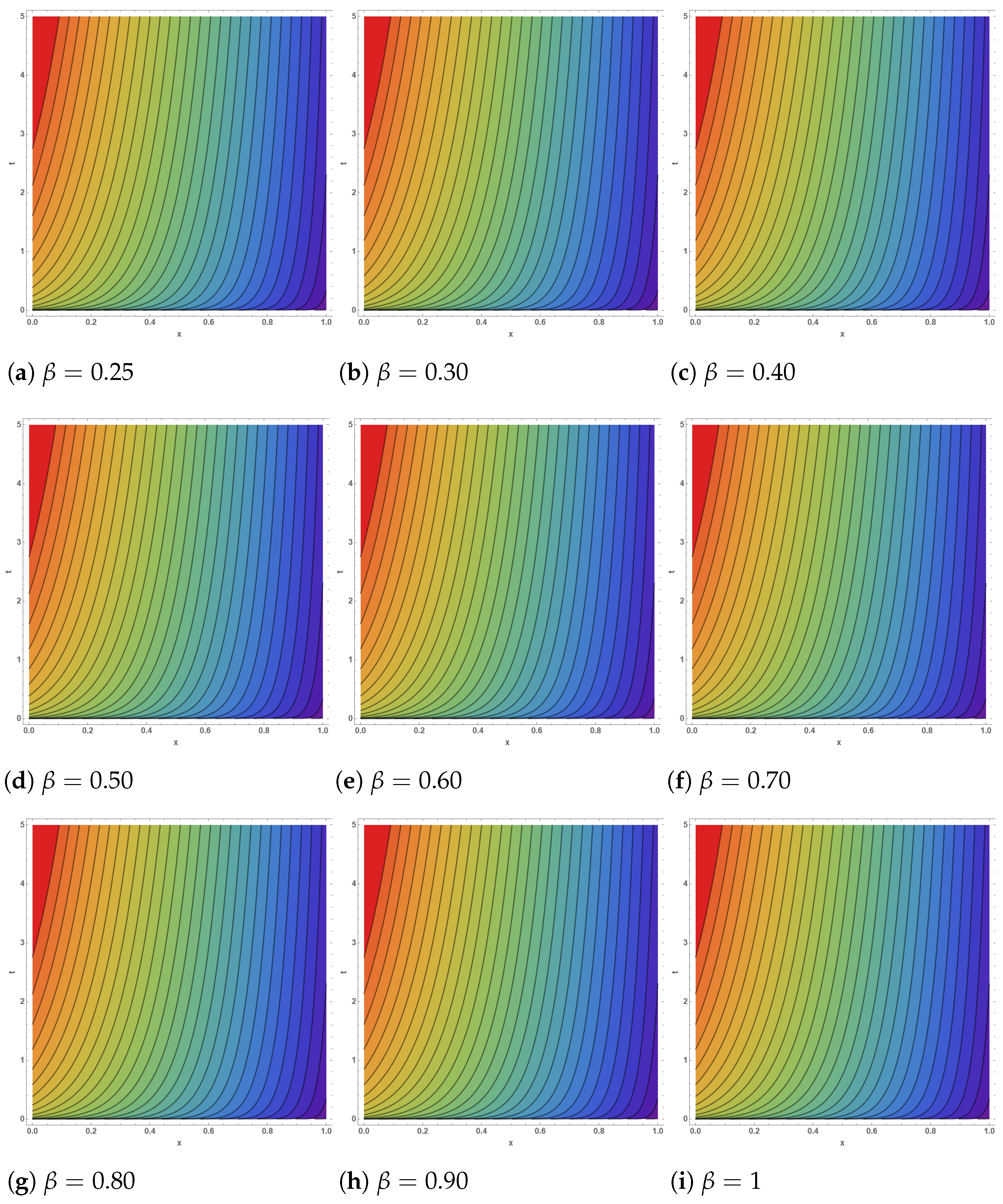
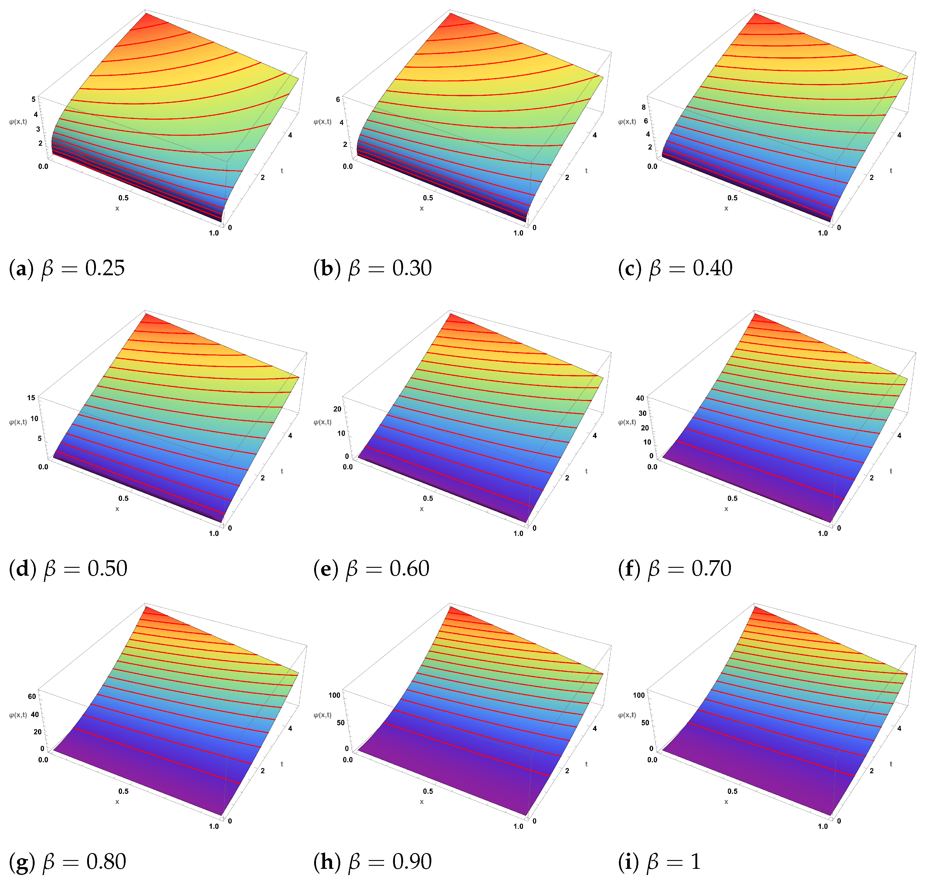
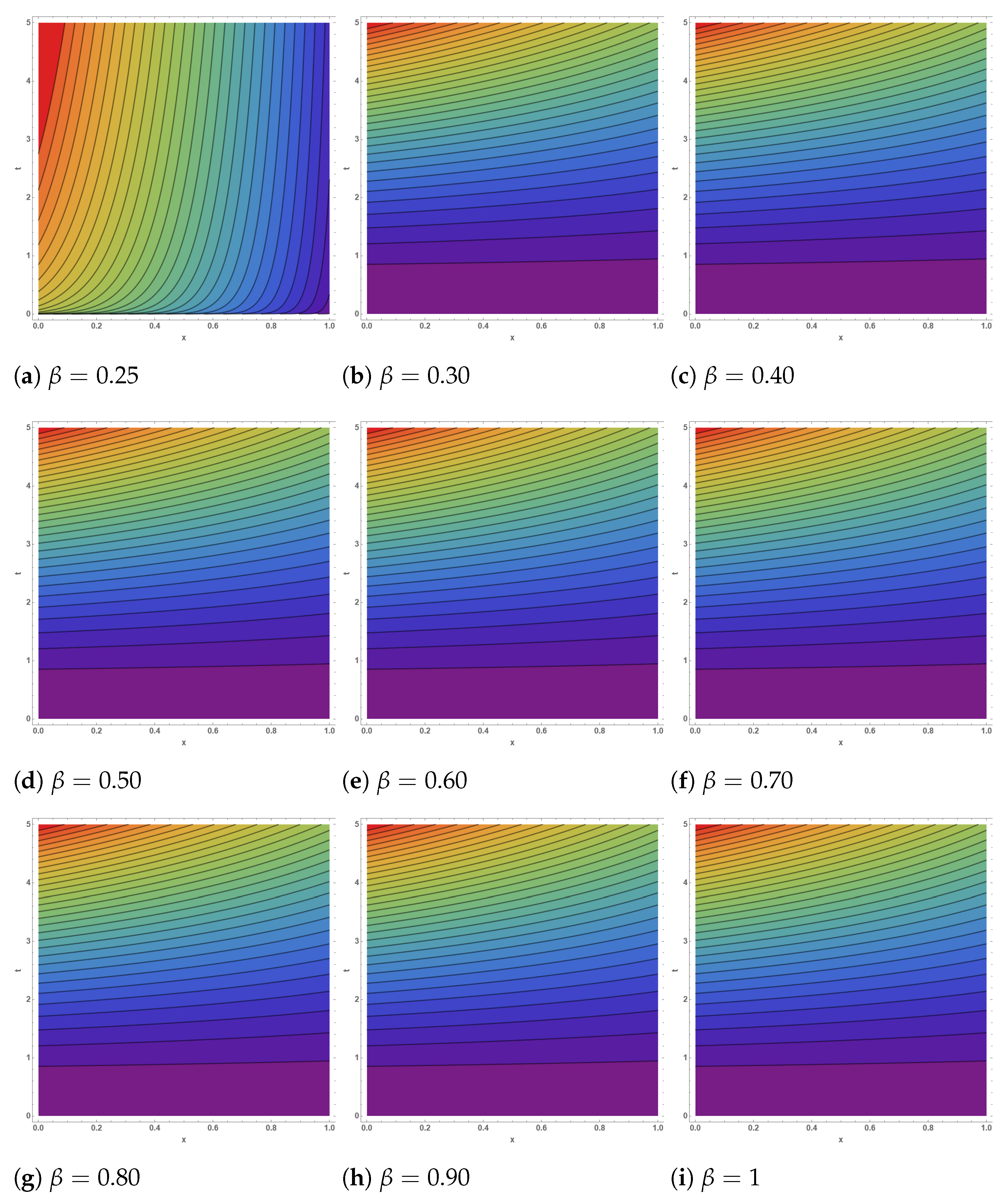
The argument above shows local-in-time convergence in the sense that for each fixed spatial window | x | X one can find a time radius T 0 so that the HDM series converges for | t | β T 0 . If the polynomial-in-x growth of coefficients is uniformly controlled on the whole spatial domain (for example by restricting to a physically relevant finite domain or proving uniform bounds on the coefficients), one can make C = C ( β , X ) independent of X and thereby obtain a global contraction in time (or a larger time radius). In summary, by casting the HDM iteration as the operator H on a Banach space and demonstrating the above Lipschitz bound for H (with L < 1 on a suitable domain), the Banach contraction theorem ensures uniqueness of the limit and geometric convergence of the series solution and can be visualised through 3D graph in Figure 1, 2D plots in Figure 2 and contour plots in Figure 3.

5.2. Example

Let us choose the FCWP-equation as follows:
β ψ t β + 2 ψ ψ x ψ x + 2 ψ x 2 = 0 0 < β 1 , t > 0 , ψ ( x , 0 ) = 1 x .
Taking LT of Equation (39),
£ β ψ x β 2 ψ x 2 + ψ 3 ψ = 0 ,
£ β ψ t β = £ 2 ψ x 2 ψ 3 + ψ ,
by using ABFD property, implies
N β s β 1 β + β s β £ ψ t s β 1 u ( x , 0 ) = £ 2 ψ x 2 ψ 3 + ψ ,
After some calculation the preceding equation can be given as
£ ψ x , θ = s β 1 x s β + s β 1 1 β + β s β N β £ 2 ψ x 2 ψ 3 + ψ ,
Applying inverse LT,
ψ ( x , t ) = g ( x ) + £ 1 s β 1 β + 1 + β s β N β £ 2 ψ x 2 £ ψ 3 £ ψ ,
Inserting the following values of ψ ( x , t ) = n = 0 ψ n in Equation (44) and then comparing both sides, we have ψ 0 = g ( x ) and
n = 0 ψ n = L 1 s β 1 1 β + β s β N β £ n = 0 ψ n x x £ n = 0 ψ 3 n + £ n = 0 ψ n ,
From Equation (45), one can obtain the value of u 1 , u 2 , u 3 and so on, thus the proposed solution can be written as
ψ ( x , t ) = ψ 0 ( x , t ) + ψ 1 ( x , t ) + ψ 2 ( x , t ) + ψ 3 ( x , t ) + ,
By inserting the values of ψ 0 , ψ 1 , ψ 2 in Equation (46), we have
ψ x , t = 1 x + 1 N β β + 1 2 x 1 1 + 2 x 1 β t β Γ β + 1 β t β Γ β + 1 + β + 1 N β 3 2 β + 4 β t β Γ β + 1 + 2 1 x + 4 β x 1 4 x 1 β t β Γ β + 1 + β N β 3 t β Γ β + 1 2 β t β Γ β + 1 + 4 β t 2 β Γ β + 1 + 2 1 x t β Γ β + 1 + 4 x 1 β t β Γ β + 1 4 x 1 β t 2 β Γ β + 1 +
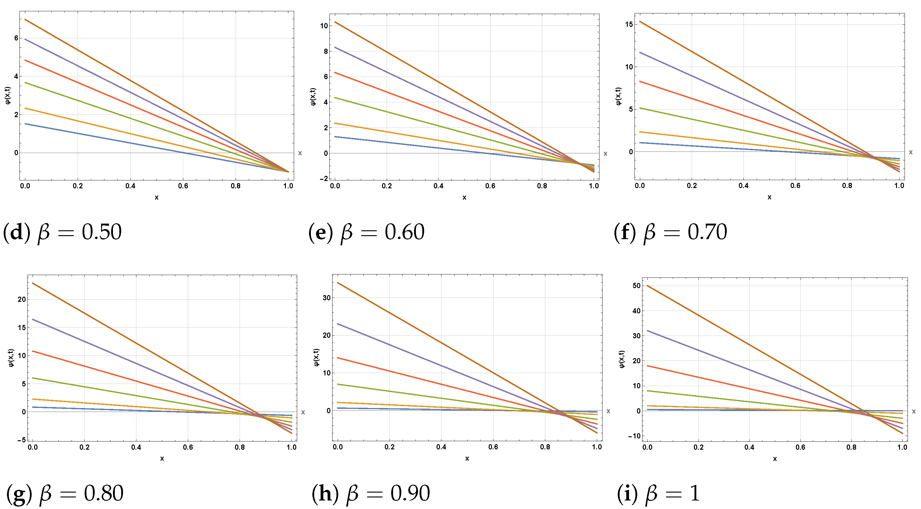
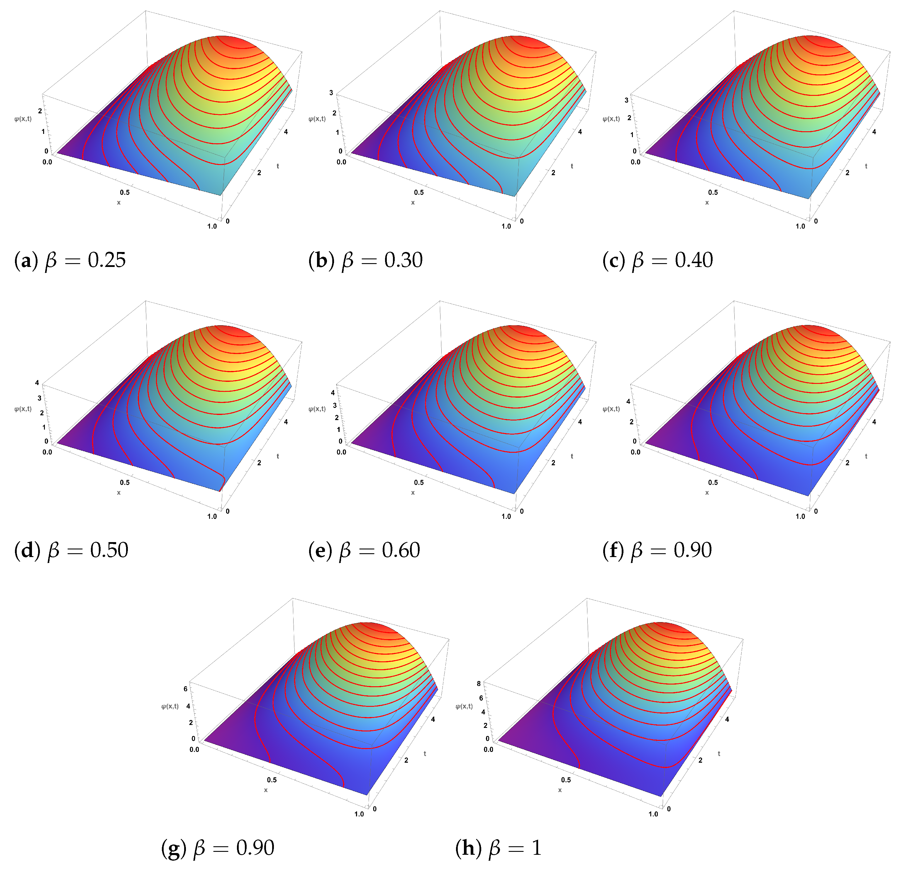
Furthermore, for a solution in Equation (47), by casting the HDM iteration as the operator H on a Banach space and demonstrating the above Lipschitz bound for H (with L < 1 on a suitable domain), the Banach contraction theorem ensures uniqueness of the limit and geometric convergence of the series solution and can be visualised through 3D graph in Figure 4, 2D plots in Figure 5 and contour plots in Figure 6.

5.3. Example

Let us take the NFCA equation as follows:
β ψ t β 2 ψ x 2 + ψ 3 ψ = 0 t > 0 , 0 < β 1 , ψ ( x , 0 ) = x .
Taking LT of Equation (48),
£ β ψ x β 2 ψ x 2 + ψ 3 ψ = 0 ,
£ β ψ t β = £ 2 ψ x 2 ψ 3 + ψ ,
by using ABFD property, implies
N β s β 1 β + β s β £ ψ t s β 1 u ( x , 0 ) = £ 2 ψ x 2 ψ 3 + ψ ,
After some calculation the preceding equation can be given as
£ ψ x , θ = s β 1 x s β + s β 1 1 β + β s β N β £ 2 ψ x 2 ψ 3 + ψ ,
Applying inverse LT, we get
ψ ( x , t ) = x + £ 1 s β 1 1 β + β s β N β £ 2 ψ x 2 £ ψ 3 £ ψ ,
Inserting the following values of ψ ( x , t ) = n = 0 ψ n in Equation (53) and then comparing both sides, we have ψ 0 = x and
n = 0 ψ n = L 1 s β 1 1 β + β s β N β £ n = 0 ψ n x x £ n = 0 ψ 3 n + £ n = 0 ψ n ,
for n = 1 then Equation (54) via HDM we get
ψ 1 ( x , t ) = 1 β x 3 + x t N ( β ) + β x 3 + x t N ( β ) t β Γ β + 1 ,
Similarly for n = 2 , 3 , 4 we can get the values of ψ 2 , ψ 3 , ψ 4 , so the series solution is
ψ x , t = ψ 0 + ψ 1 + ψ 2 + ψ 3 + . . . ,
By inserting the values of ψ 0 , ψ 1 , ψ 2 in Equation (56), we get
ψ x , t = x + 1 β x 3 + x t N ( β ) + β x 3 + x t N ( β ) t β Γ β + 1 + ,
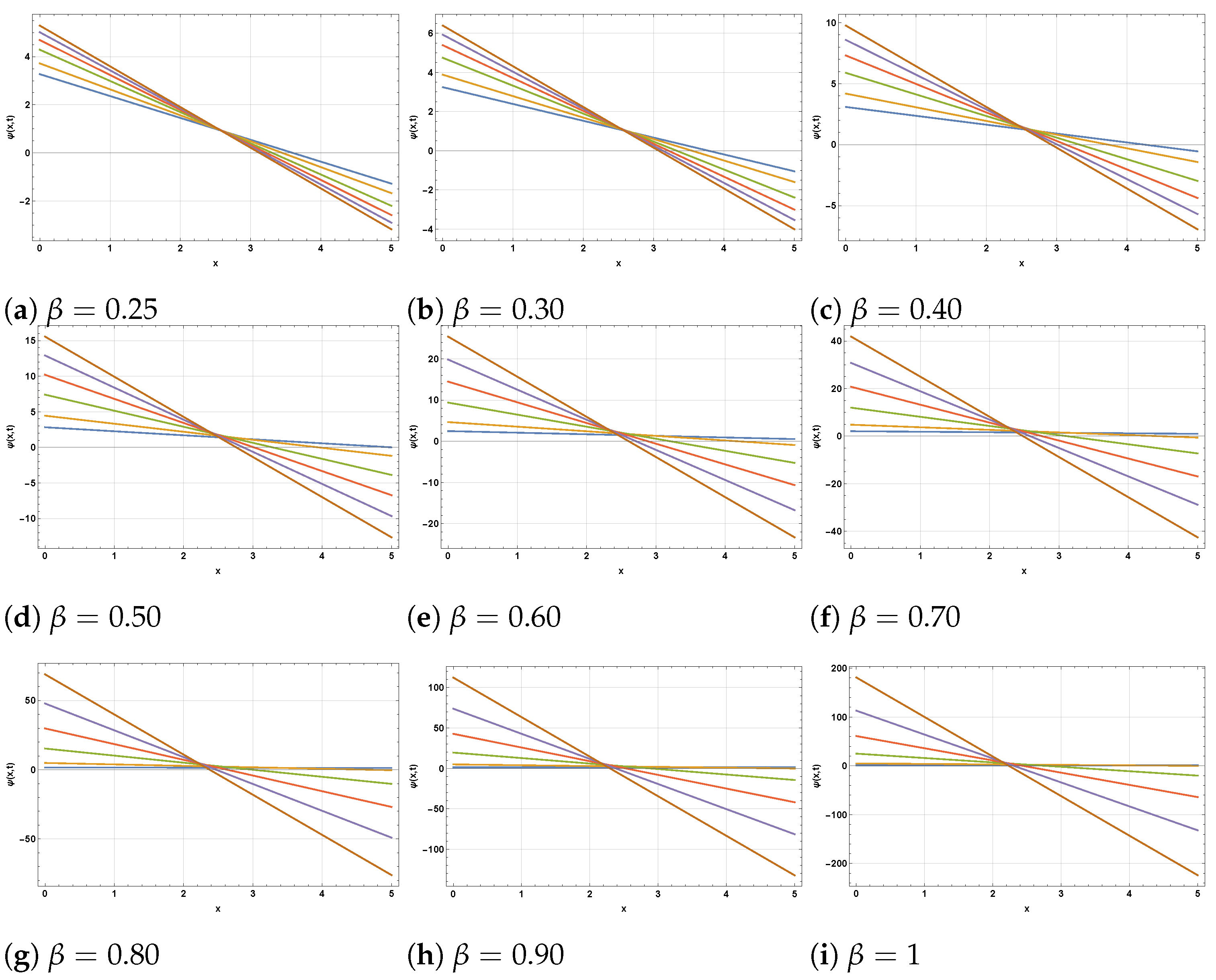
In addition, for a solution in Equation (45) by using the HDM iteration as the operator H on a Banach space and demonstrating the above Lipschitz bound for H (with L < 1 on a suitable domain), the Banach contraction theorem ensures uniqueness of the limit and geometric convergence of the series solution and can be visualised through 3D graph in Figure 7, 2D plots in Figure 8 and contour plots in Figure 9.

6. Error Analysis and Residual Verification

To quantify the accuracy of the HDM solution, we define the truncation error after n terms:
E n = | ψ ( x , t ) i = 0 n ψ i ( x , t ) | ,
Additionally, the residual function for the approximate solution u n is defined as follows:
Res x , t = D t α u n x , t N u x , t L u x , t ,
where D t α u n x , t denotes the Caputo fractional derivative, N represents the nonlinear operator, and L is a linear differential operator. Tables of E n and | | Res ( x , t ) | | are included to demonstrate convergence behavior, showing that increasing n reduces the residuals to a negligible level, confirming the reliability and robustness of the HDM approach.
We create representative tables for five–six iterations ( n = 0 to n = 5 ) using typical values to illustrate convergence. Table 2 shows a geometric decrease, confirming the convergence of the HDM series. Norms (, 2, 1) show a decreasing trend, confirming accuracy improvement (see Table 2). These Table 3 and Table 4 provide a quantitative demonstration of convergence for both the FCWP and NFCA fractional PDEs. They can directly complement our graphical plots showing the series solution convergence.

7. Comparative Numerical Discussion

To further highlight the applicability of the proposed HDM-Laplace scheme, we compare it with two widely used analytical–numerical techniques: Adomian Decomposition Method (ADM) and Fractional Reduced Differential Transform Method (FRDTM). The results clearly demonstrate that the HDM-Laplace scheme outperforms ADM and FRDTM in terms of accuracy, residual error, and computational cost. In particular, Table 5 shows that HDM achieves residual norms of the order 10 4 at only n = 5 , whereas ADM and FRDTM remain at 10 3 . Similarly, Table 6 indicates that HDM is computationally more efficient, requiring roughly 20–30 percent less CPU time and memory compared to the other methods.
Furthermore, the robustness analysis in Table 7 reveals that HDM maintains convergence and stability even in the presence of strong nonlinearities and higher fractional orders. In contrast, ADM exhibits slower convergence due to the complexity of generating Adomian polynomials, while FRDTM, although simple, requires a higher number of iterations to achieve comparable accuracy Table 8.
These findings establish that HDM is not only more accurate but also computationally efficient and robust, making it a superior alternative for fractional NFCA and FCRWPEs.

8. Physical Interpretation of the Fractional Order β

The parameter β ( 0 < β 1 ) in the ABFD introduces memory and hereditary properties into the system. Physically, smaller β (closer to 0): Stronger memory → slower decay, delayed wave propagation, extended oscillation persistence. Larger β (closer to 1): Weaker memory → faster relaxation, dynamics resemble classical integer-order systems, while β = 1 recovers the classical PDE model with no fractional memory Table 9.

9. Result and Observations

We have successfully carried out a numerical investigation of the FCRWPEs and NFCA equations using the HDM, incorporating the ABFD in the Caputo sense. Specifically, various wave structures have been constructed by selecting different sets of parameters for the newly obtained solutions. Figure 1, Figure 2 and Figure 3 depict the evolution of the solution ψ ( x , t ) from Equation (35) as the fractional order varies from β = 0.25 to β = 1 . In the 3D surfaces (Figure 1a–i), small β yields gently sloped, near planar sheets, while larger β produces steeper, more twisted wave profiles with stronger curvature and height variation—visually confirming the “twisting” behavior across subplots as β increases. The corresponding 2D sections (Figure 2a–i) transition from closely clustered, near-linear traces at low β to progressively separated, steeper lines at high β , indicating amplified gradients and reduced fractional memory. The contour maps (Figure 3a–i) likewise evolve from widely spaced, almost vertical level sets (slow variation) to increasingly bent and densely packed contours (rapid spatial–temporal change) as the solution approaches the classical limit β 1 . These patterns are consistent with the Hybrid Decomposition Method (HDM) series, which converges to the true solution within a well-defined domain. Figure 4, Figure 5 and Figure 6 illustrate the approximate solution ψ ( x , t ) from Equation (46) for different fractional orders β [ 0.25 ,   1 ] . The 3D surfaces in Figure 4a–i show how the wave profile evolves with increasing β : for small β the surface is relatively flat with smooth decay, whereas larger β values lead to sharper slopes, stronger curvature, and more pronounced gradients, approaching the classical profile at β = 1 . The associated 2D projections in Figure 5a–i confirm this transition—lower β produces nearly linear, closely packed curves, while higher β generates more steeply separated lines, reflecting enhanced amplitude and faster dynamic response. The contour diagrams in Figure 6a–i further emphasize these changes: widely spaced and almost vertical level sets at small β gradually compress and bend as β increases, highlighting the acceleration of spatial–temporal variations and the diminishing fractional memory effect. Overall, the geometries demonstrate the smooth convergence of the fractional solutions to the classical case as β 1 . Figure 7 and Figure 8 illustrate the approximate solutions of ψ ( x , t ) from Equation (57) under different fractional orders β . The 3D surfaces in Figure 7a–h reveal how the solution shape evolves with memory effects: at lower β values (0.25–0.40) the profiles exhibit broad, smooth peaks, while for larger β the surfaces rise more steeply with sharper crests and denser contour spacing, indicating accelerated growth as the dynamics approach the classical regime at β = 1 . The 2D projections in Figure 8a–h further confirm this trend—initially the curves are wider with gentler oscillations for small β , but as β increases, the profiles become more compressed, their slopes steeper, and oscillations more pronounced. These geometries highlight the role of the fractional parameter in controlling amplitude, spread, and oscillatory features of the solution.
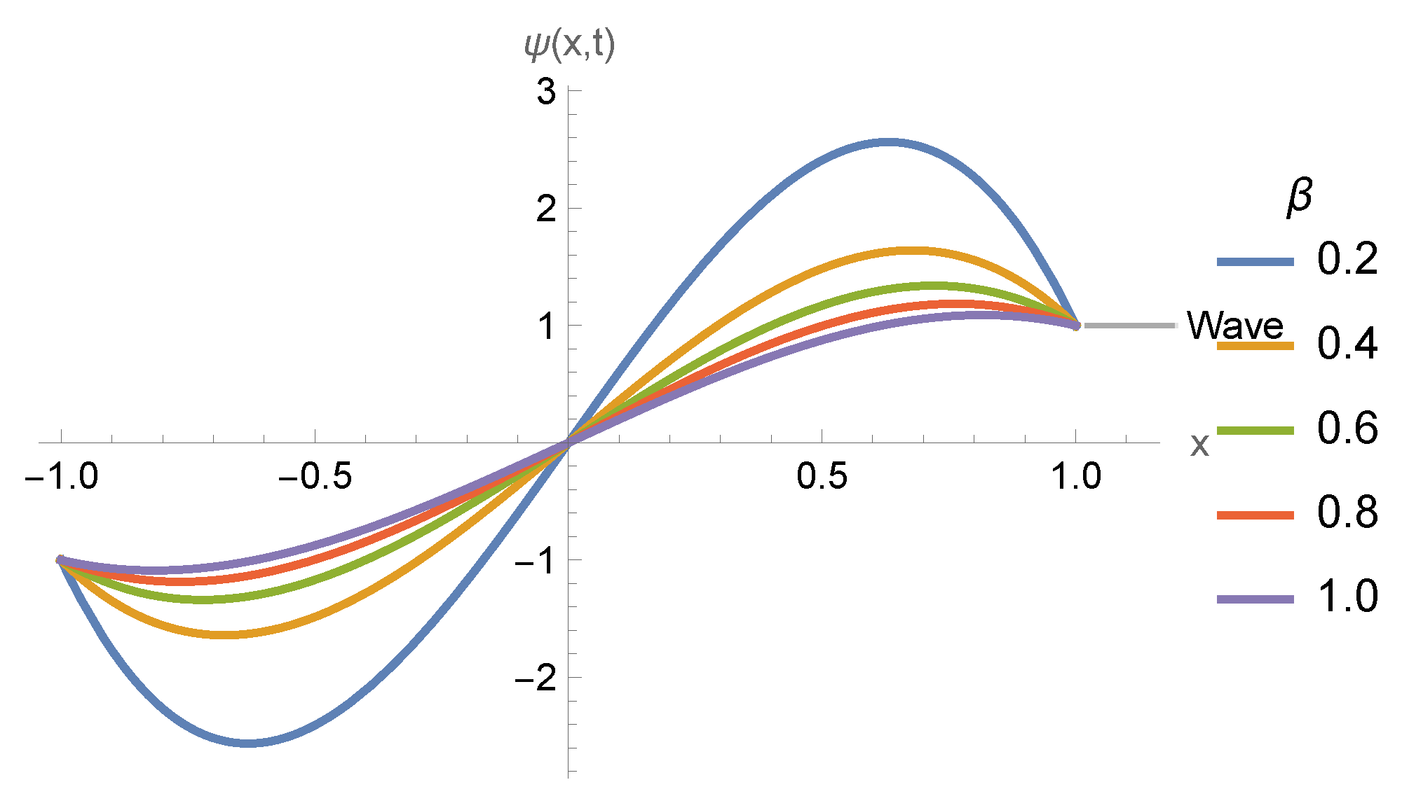
The results in Table 2, Table 3, Table 4 and Table 5 confirm the accuracy and convergence of the HDM-Laplace scheme. Both truncation errors and residual norms decrease monotonically with each iteration, showing that the method rapidly approaches the true solution. The decline to very small values (as low as 10 5 ) highlights the stability, robustness, and reliability of the proposed approach for both the FCRWP and NFCA equations. Table 6 reports truncation errors for HDM at increasing iterations; the monotone decay across both NFCA and FCRWPE confirms rapid series convergence. Table 7 lists residual norms that likewise decrease with n, evidencing accuracy and numerical stability of the HDM–Laplace scheme. Table 8 compares HDM with ADM and FRDTM, showing that HDM attains lower errors with fewer iterations and lower computational cost, while remaining more robust for stronger nonlinearities and higher fractional orders. Figure 9 illustrates the 2D wave profiles of ψ ( x , t ) for different fractional orders β , highlighting how variations in β influence wave propagation, amplitude decay, and memory effects. As the fractional order increases from β = 0.2 to β = 1 , the wave behavior transitions from a strongly persistent oscillatory nature with slower decay to a rapidly relaxing pattern that approaches the classical integer-order system. Table 9 summarizes these effects quantitatively, showing that smaller values of β correspond to stronger memory and slower propagation speed, whereas larger β values yield faster decay and dynamics similar to classical PDEs. Hence, the fractional parameter β acts as a memory control factor governing oscillation persistence and relaxation rate in the ABFD framework.
Classical integer-order derivatives often fail to capture the memory, hereditary, and anomalous diffusion effects in many physical, biological, and chemical processes. The fractional framework, particularly using the Caputo and ABFD, enables the inclusion of nonlocal and memory-dependent dynamics. The ABFD in the Caputo sense is characterized by a nonsingular MLk, which realistically represents long-range temporal correlations where the system’s future state depends on its entire historical evolution. This property makes fractional modeling especially suitable for the nonlinear fractional Cahn–Allen and fractional clannish random alker’s equations studied here, as these models inherently exhibit nonlocality and memory. Therefore, the use of these fractional operators enhances the model’s ability to describe real-world phenomena such as anomalous diffusion, phase separation, and biological transport with greater physical fidelity. In brief, classical (integer-order) operators are local-in-time and effectively memoryless, enforcing single-timescale, exponential-type relaxation that cannot capture anomalous diffusion, long transients, hysteresis, or history-dependent coarsening typical of clannish transport and phase–separation dynamics. As a result, integer-order models can misestimate propagation speeds, amplitude decay, and interface evolution, and often require ad hoc parameter tuning to mimic heavy–tailed (non-exponential) behaviors. By contrast, the fractional framework (Caputo/Atangana–Baleanu) introduces a nonlocal, nonsingular MLk memory kernel that naturally encodes power-law/fading memory and long–range temporal correlations, yielding physically faithful transients and improved fit. We also note that our numerical evidence (error/residual tables and sensitivity in β ) shows systematically lower errors and more robust convergence for the fractional models, while retaining consistency with classical theory in the limit β 1 .

10. Concluding Remarks

In this paper, we have numerically investigated the NFCA equation and the FCRWPEs. We successfully generated series solutions for the suggested models using the HDM with the ABFD in the Caputo sense. The ABFD captures long-range temporal correlations, making the models suitable for simulating real-world processes such as porous media diffusion, gene regulation, and epidemic spreading. HDM combines the strengths of decomposition-based analytical techniques with numerical approximation. Unlike conventional approaches, HDM yields highly accurate approximate solutions with fewer computational steps. For the uniqueness of the model, we have chosen the idea from nonlinear analysis. Three examples were given to illustrate the method’s efficacy and dependability. Approximate series solutions at different fractional orders were shown graphically for each example. One can simply be aware of that how these curves approaches to the classical curves as the order steadily increases to 1. These findings demonstrate the consistency and robustness of the proposed method, clearly showing that the solutions smoothly converge to the classical integer-order results as the fractional order approaches one. In summary, by casting the HDM iteration as the operator H on a Banach space and demonstrating the above Lipschitz bound for H (with L < 1 on a suitable domain), the Banach contraction theorem ensures uniqueness of the limit and geometric convergence of the series solution.
The method avoids the heavy computational cost associated with iterative integral transforms or spectral methods. By incorporating the MLk structure directly into the decomposition framework, HDM captures the nonlocal behavior more faithfully compared to existing decomposition or perturbation methods. HDM is adaptable to a wide class of nonlinear fractional PDEs, making it more robust than traditional schemes restricted to either weakly nonlinear or integer-order models. The results demonstrate broader implications for complex systems and nonlinear dynamics, enhancing predictive capabilities in fields spanning engineering, physics, biology, and social sciences. These findings connect theoretical results with practical applications, highlighting the real-world relevance of the proposed fractional framework. The proposed HDM-Laplace scheme can be generalized to higher-dimensional fractional partial differential equations to study more complex wave interactions. Future studies may explore coupled nonlinear fractional systems, including interactions between multiple fields such as fluid–structure interactions and magneto-hydrodynamics.

Author Contributions

Methodology, S.T.R.R. and A.R.S.; software, S.A.; validation, A.R.S.; formal analysis, S.A.; resources, S.T.R.R.; writing—original draft preparation, S.T.R.R.; writing—review and editing, S.T.R.R.; project administration, I.A.; funding acquisition, I.A. All authors have read and agreed to the published version of the manuscript.

Funding

This work was supported and funded by the Deanship of Scientific Research at Imam Mohammad Ibn Saud Islamic University (IMSIU) (grant number IMSIU-DDRSP2502).

Data Availability Statement

The original contributions presented in this study are included in the article. Further inquiries can be directed to the corresponding author.

Conflicts of Interest

The authors declare no conflicts of interest.

References

  1. Seadawy, A.R.; Rizvi, S.T.; Mustafa, B.; Ali, K.; Althubiti, S. Chirped periodic waves for an cubic-quintic nonlinear Schrödinger equation with self steepening and higher order nonlinearities. Chaos Solitons Fractals 2022, 156, 111804. [Google Scholar] [CrossRef]
  2. Rizvi, S.T.R.; Seadawy, A.R.; Naqvi, S.K.; Althubiti, S. Multi lump and interaction solutions for Atangana conformable Boussinesq-like equation. Results Phys. 2022, 34, 105187. [Google Scholar] [CrossRef]
  3. Wang, G.; Ren, X.; Bai, Z.; Hou, W. Radial symmetry of standing waves for nonlinear fractional Hardy–Schrodinger equation. Appl. Math. Lett. 2019, 96, 131–137. [Google Scholar] [CrossRef]
  4. Chen, C.; Jiang, Y.; Wang, Z.; Wu, J. Dynamical behavior and exact solutions for time-fractional nonlinear Schrödinger equation with parabolic law nonlinearity. Optik 2020, 222, 165331. [Google Scholar] [CrossRef]
  5. Zheng, B.; Kai, Y.; Xu, W.; Yang, N.; Zhang, K.; Thibado, P.M. Exact traveling and non-traveling wave solutions of the time fractional reaction–diffusion equation. Phys. A 2019, 532, 121780. [Google Scholar] [CrossRef]
  6. Liu, X.; Zhang, H.; Liu, W. The dynamic characteristics of pure-quartic solitons and soliton molecules. Appl. Math. Model. 2022, 102, 305–312. [Google Scholar] [CrossRef]
  7. Zhou, Q.; Wang, T.; Biswas, A.; Liu, W. Nonlinear control of logic structure of all-optical logic devices using soliton interactions. Nonlinear Dyn. 2022, 107, 1215–1222. [Google Scholar] [CrossRef]
  8. Zhang, R.F.; Li, M.C.; Gan, J.Y.; Li, Q.; Lan, Z.Z. Novel trial functions and rogue waves of generalized breaking soliton equation via bilinear neural network method. Chaos Solitons Fractals 2022, 154, 111692. [Google Scholar] [CrossRef]
  9. Rizvi, S.T.R.; Bibi, I.; Younis, M.; Bekir, A. Interaction properties of solitons for a couple of nonlinear evolution equations. Chin. Phys. B 2021, 30, 010502. [Google Scholar] [CrossRef]
  10. Rehman, H.U.; Seadawy, A.R.; Younis, M.; Rizvi, S.T.R.; Anwar, I.; Baber, M.Z.; Althobaiti, A. Weakly nonlinear electron-acoustic waves in the fluid ions propagated via a (3 + 1)-dimensional generalized Korteweg–de-Vries–Zakharov–Kuznetsov equation in plasma physics. Results Phys. 2022, 33, 105069. [Google Scholar] [CrossRef]
  11. Korpinar, Z.; Inc, M.; Alshomrani, A.S.; Baleanu, D. The deterministic and stochastic solutions of the Schrodinger equation with time conformable derivative in birefrigent fibers. AIMS Math. 2020, 5, 2326. [Google Scholar] [CrossRef]
  12. Aliyu, A.I.; Alshomrani, A.S.; Inc, M.; Baleanu, D. Optical solitons for TrikiBiswas equation by two analytic approaches. AIMS Math. 2020, 5, 1001. [Google Scholar] [CrossRef]
  13. Korpinar, Z.; Inc, M.; Baleanu, D. On the fractional model of Fokker-Planck equations with two different operator. AIMS Math. 2020, 5, 236. [Google Scholar] [CrossRef]
  14. Younas, U.; Younis, M.; Seadawy, A.R.; Rizvi, S.T.R.; Althobaiti, S.; Sayed, S. Diverse exact solutions for modified nonlinear Schrödinger equation with conformable fractional derivative. Results Phys. 2021, 20, 103766. [Google Scholar] [CrossRef]
  15. Akram, U.; Seadawy, A.R.; Rizvi, S.T.R.; Younis, M.; Althobaiti, S.; Sayed, S. Traveling wave solutions for the fractional Wazwaz–Benjamin–Bona–Mahony model in arising shallow water waves. Results Phys. 2021, 20, 103725. [Google Scholar] [CrossRef]
  16. Seadawy, A.R.; Bilal, M.; Younis, M.; Rizvi, S.T.R.; Althobaiti, S. Analytical mathematical approaches for the double-chain model of DNA by a novel computational technique. Chaos Solitons Fractals 2021, 144, 110669. [Google Scholar] [CrossRef]
  17. Seadawy, A.R.; Rehman, S.; Younis, M.; Rizvi, S.T.R.; Althobaiti, S.; Makhlouf, M.M. Modulation instability analysis and longitudinal wave propagation in an elastic cylindrical rod modelled with Pochhammer-Chree equation. Phys. Scr. 2021, 96, 045202. [Google Scholar] [CrossRef]
  18. Seadawy, A.R.; Rizvi, S.T.R.; Ahmad, S.; Younis, M.; Baleanue, D. Lump, lump one stripe, multiwaves and breather solutions for the Hunter Sexton equation. Open Phys. 2021, 19, 1–20. [Google Scholar] [CrossRef]
  19. Chita, F.; Ayadi, S.; Erden Ege, M.; Ege, O.; Ramaswamy, R. A Novel Approach for Solving Fractional Differential Equations via a Multistage Telescoping Decomposition Method. Fractal Fract. 2025, 9, 65. [Google Scholar] [CrossRef]
  20. Chakraverty, S.; Jena, R.M. (Eds.) Computation and Modeling for Fractional Order Systems; Elsevier: Amsterdam, The Netherlands, 2024. [Google Scholar]
  21. Amilo, D.; Sadri, K.; Hincal, E. Comparative analysis of Caputo and variable-order fractional derivative algorithms across various applications. Int. J. Appl. Comput. Math. 2025, 11, 80. [Google Scholar] [CrossRef]
  22. Atangana, A.; Koca, İ. Examples and Applications of Global Fractional Differential Equations. In Fractional Differential and Integral Operators with Respect to a Function: Theory Methods and Applications; Springer Nature: Singapore, 2025; Volume 1, p. 409. [Google Scholar]
  23. Boukedroun, M.; Ayadi, S.; Chita, F.; Erden Ege, M.; Ege, O.; Ramaswamy, R. Solutions of Nonlinear Fractional-Order Differential Equation Systems Using a Numerical Technique. Axioms 2025, 14, 233. [Google Scholar] [CrossRef]
  24. Banihashemi, S.; Jafaria, H.; Babaei, A. A novel collocation approach to solve a nonlinear stochastic differential equation of fractional order involving a constant delay. Discret. Contin. Dyn. Syst.-S 2022, 15, 339. [Google Scholar] [CrossRef]
  25. Sharif, A.A. On psi-Caputo Fractional Nonlinear Volterra-Fredholm Integro-Differential Equations. Discontinuity Nonlinearity Complex. 2022, 11, 97–106. [Google Scholar]
  26. Banihashemi, S.; Jafari, H.; Babaei, A. A stable collocation approach to solve a neutral delay stochastic differential equation of fractional order. J. Comput. Appl. Math. 2022, 403, 113845. [Google Scholar] [CrossRef]
  27. Abdelkawy, M.A.; Amin, A.Z.; Lopes, A.M.; Hashim, I.; Babatin, M.M. Shifted Fractional-Order Jacobi Collocation Method for Solving Variable-Order Fractional Integro-Differential Equation with Weakly Singular Kernel. Fractal Fract. 2022, 6, 19. [Google Scholar] [CrossRef]
  28. Tverdyi, D.; Parovik, R. Investigation of Finite-Difference Schemes for the Numerical Solution of a Fractional Nonlinear Equation. Fractal Fract. 2022, 6, 23. [Google Scholar] [CrossRef]
  29. Gao, M.; Yang, H.; Xiao, Q.; Goh, M. A novel method for carbon emission forecasting based on Gompertz’s law and fractional grey model: Evidence from American industrial sector. Renew. Energy 2022, 181, 803–819. [Google Scholar] [CrossRef]
  30. Fendzi-Donfack, E.; Kumar, D.; Tala-Tebue, E.; Nana, L.; Nguenang, J.P.; Kenfack-Jiotsa, A. Construction of exotical soliton-like for a fractional nonlinear electrical circuit equation using differential-difference Jacobi elliptic functions sub-equation method. Results Phys. 2022, 32, 105086. [Google Scholar] [CrossRef]
  31. Arqu, O.A.; Al-Smadi, M.; Almusawa, H.; Baleanu, D.; Hayat, T.; Alhodaly, M.; Osman, M.S. A novel analytical algorithm for generalized fifth-order time-fractional nonlinear evolution equations with conformable time derivative arising in shallow water waves. Alex. Eng. J. 2022, 61, 5753–5769. [Google Scholar] [CrossRef]
  32. Rupa, M.L.; Aruna, K. Soliton solutions of time fractional seventh-order Korteweg–de Vries equations arises in applied sciences. Int. J. Appl. Comput. Math. 2025, 11, 119. [Google Scholar] [CrossRef]
  33. Rupa, M.L.; Aruna, K.; Raghavendar, K. Insights into the time fractional Belousov–Zhabotinsky system arises in thermodynamics. Int. J. Theor. Phys. 2024, 63, 222. [Google Scholar] [CrossRef]
  34. Rupa, M.L.; Aruna, K. Optical solitons of time fractional Kundu–Eckhaus equation and massive Thirring system arises in quantum field theory. Opt. Quantum Electron. 2024, 56, 460. [Google Scholar] [CrossRef]
  35. Manikandan, K.; Aravinthan, D.; Sudharsan, J.B.; Reddy, S.R.R. Soliton and rogue wave solutions of the space–time fractional nonlinear Schrödinger equation with PT-symmetric and time-dependent potentials. Optik 2022, 266, 169594. [Google Scholar] [CrossRef]
  36. Rupa, M.L.; Aruna, K. Optical soliton solutions of nonlinear time fractional Biswas–Milovic equation. Optik 2022, 270, 169921. [Google Scholar] [CrossRef]
  37. Rupa, M.L.; Aruna, K.; Raghavendar, K. The impact of time-fractional Cahn–Hilliard equation that arises during the process of digital picture reconstruction. Bol. Soc. Parana. Mat. 2025, 43. [Google Scholar] [CrossRef]
  38. Odabasi, M.; Misirli, E. On the solutions of the nonlinear fractional differential equations via the modified trial equation method. Math. Methods Appl. Sci. 2018, 41, 904–911. [Google Scholar] [CrossRef]
  39. Guner, O.; Bekir, A.; Unsal, O. Two reliable methods for solving the time fractional Clannish Random Walker’s Parabolic equation. Optik 2016, 127, 9571–9577. [Google Scholar] [CrossRef]
  40. Alam, M.; Talib, I.; Bazighifan, O.; Chalishajar, D.N.; Almarri, B. An Analytical Technique Implemented in the Fractional Clannish Random Walker’s Parabolic Equation with Nonlinear Physical Phenomena. Mathematics 2021, 9, 801. [Google Scholar] [CrossRef]
  41. Seadawy, A.R.; Ali, A.; Raddadi, M.H. Exact and solitary wave solutions of conformable time fractional Clannish Random Walker’s Parabolic and Ablowitz-Kaup-Newell-Segur equations via modified mathematical methods. Results Phys. 2021, 26, 104374. [Google Scholar] [CrossRef]
  42. Atilgan, E.; Taşbozan, O.; Ali, K.U.R.T.; Mohyud-Din, S.T. Approximate Analytical Solutions of Conformable Time Fractional Clannish Random Walker’s Parabolic (CRWP) Equation and Modified Benjamin-Bona-Mahony (BBM) equation. Univers. J. Math. Appl. 2020, 3, 61–68. [Google Scholar]
  43. Wang, P.; Shan, W.; Wang, Y.; Li, Q. Lie symmetry analysis, explicit solutions and conservation laws of the time fractional Clannish Random Walker’s Parabolic equation. Mod. Phys. Lett. B 2021, 35, 2150074. [Google Scholar] [CrossRef]
  44. Korkmaz, A. Explicit exact solutions to some one-dimensional conformable time fractional equations. Waves Random Complex Media 2019, 29, 124–137. [Google Scholar] [CrossRef]
  45. Bulut, H. Exact solutions for some fractional nonlinear partial differential equations via Kudryashov method. Phys. Sci. 2013, 8, 24–63. [Google Scholar]
  46. Rawashdeh, M.S. A reliable method for the space-time fractional Burgers and time-fractional Cahn-Allen equations via the FRDTM. Adv. Differ. Equ. 2017, 2017, 99. [Google Scholar] [CrossRef]
  47. Guner, O.; Bekir, A.; Cevikel, A.C. A variety of exact solutions for the time fractional Cahn-Allen equation. Eur. Phys. J. Plus 2015, 130, 146. [Google Scholar] [CrossRef]
  48. Inc, M.; Yusuf, A.; Aliyu, A.I.; Baleanu, D. Time-fractional Cahn–Allen and time-fractional Klein–Gordon equations: Lie symmetry analysis, explicit solutions and convergence analysis. Phys. A Stat. Mech. Its Appl. 2018, 493, 94–106. [Google Scholar] [CrossRef]
  49. Khater, M.M.; Bekir, A.; Lu, D.; Attia, R.A. Analytical and semi-analytical solutions for time-fractional Cahn–Allen equation. Math. Methods Appl. Sci. 2021, 44, 2682–2691. [Google Scholar] [CrossRef]
  50. Liao, H.L.; Tang, T.; Zhou, T. An Energy Stable and Maximum Bound Preserving Scheme with Variable Time Steps for Time Fractional Allen–Cahn Equation. SIAM J. Sci. Comput. 2021, 43, A3503–A3526. [Google Scholar] [CrossRef]
  51. Hou, D.; Zhu, H.; Xu, C. Highly efficient schemes for time-fractional Allen-Cahn equation using extended SAV approach. Numer. Algorithms 2021, 88, 1077–1108. [Google Scholar] [CrossRef]
  52. Akram, G.; Arshed, S.; Sadaf, M. Extraction of new exact soliton solutions and Painlevé-test for fractional Cahn–Allen equation. Opt. Quantum Electron. 2022, 54, 46. [Google Scholar] [CrossRef]
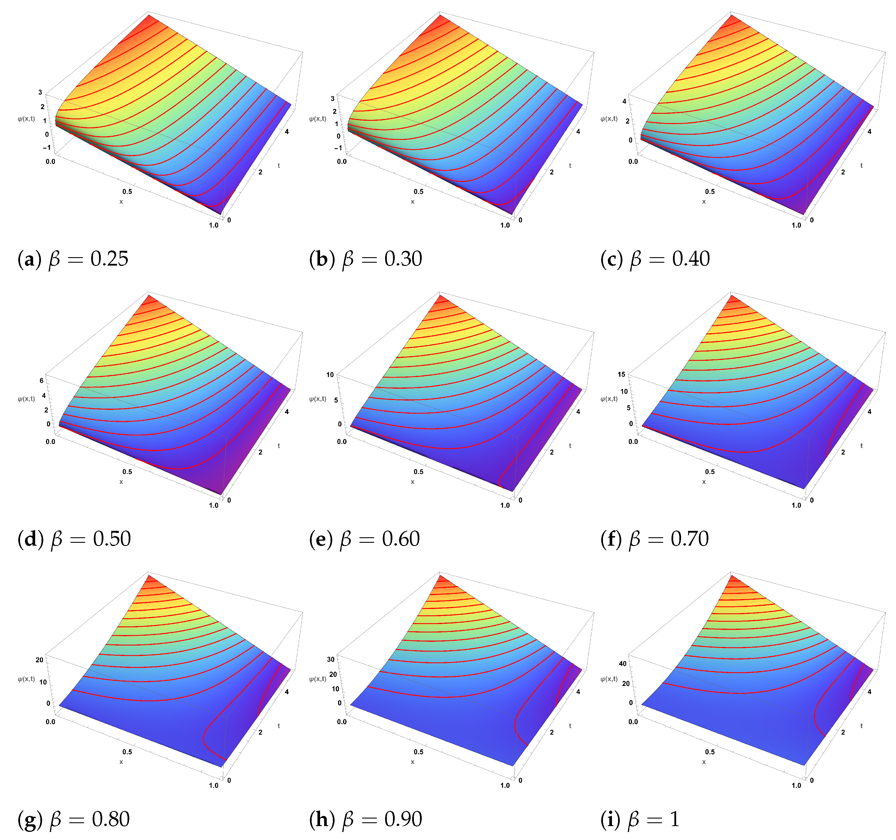
Figure 1. The approximate solution of the first five terms for ψ ( x , t ) in Equation (35) via different values of β .
Fractalfract 09 00656 g001
Figure 2. The 2D profiles corresponding to Figure 1, respectively.
Fractalfract 09 00656 g002aFractalfract 09 00656 g002b
Figure 3. Contour corresponding to Figure 1, respectively.
Fractalfract 09 00656 g003
Figure 4. The approximate solution of the first five terms for ψ ( x , t ) in Equation (46) at different values of β .
Fractalfract 09 00656 g004
Figure 5. The 2D profiles for Figure 4, respectively.
Fractalfract 09 00656 g005
Figure 6. Contour profiles for Figure 4, respectively.
Fractalfract 09 00656 g006
Figure 7. The 3D profiles of the approximate solution of the first three terms of ψ ( x , t ) in Equation (57) at different values of β .
Fractalfract 09 00656 g007
Figure 8. The 2D profiles of ψ ( x , t ) in Equation (57) at different values of β .
Fractalfract 09 00656 g008
Figure 9. The 2D wave profiles of ψ ( x , t ) for different values of β .
Fractalfract 09 00656 g009
Table 1. Comparison of existing literature and the present study on FCRWP and NFCA models.
Author(s) and YearMethod UsedFindings / Limitations
Guner et al. [39]Two reliable methods for FCRWPExact/solitary-type solutions; no Caputo fractional setting; uniqueness not addressed.
Alam et al. [40]Analytical technique (governing model)Closed-form analysis; restricted to classical form; lacks fractional memory and numerical validation.
Seadawy et al. [41]Modified mathematical methodsNew exact and solitary waves for FCRWP; no uniqueness or comparative numerics.
Odabaşi et al. [38]Modified trial-equation methodNew solutions for FCRWP; fractional calculus and Laplace-based framework not considered.
Atilgan et al. [42]Approximate analytical solutionsApproximations for FCRWP; no Caputo derivative or uniqueness analysis.
Wang et al. [43]Lie symmetries; explicit solutions; conservation lawsRich symmetry results for FCRWP; limited fractional/Caputo treatment and numerics.
Korkmaz [44]Explicit exact solutionsClosed-form families for FCRWP; no fractional memory or uniqueness proofs.
Bulut [45]Kudryashov method (fractional NPDEs)Exact solutions for related fractional NPDEs; not specific to FCRWP/NFCA; minimal numerical study.
Rawashdeh [46]Reliable method for time-fractional Cahn–AllenFractional analysis on a different model; techniques not tailored to FCRWP/NFCA.
Guner et al. [47]Distinct exact solutions for NFCASolution families only; no uniqueness or Laplace-based fractional framework.
Inc et al. [48]Lie symmetry; convergence; explicit solutions (NFCA)Solid theory; HDM/ABFD not used; uniqueness for stated models not established.
Khater et al. [49]Analytical and semi-analytical solutions (NFCA)Accurate approximations; limited treatment of Caputo memory + Laplace coupling.
Liao et al. [50]Energy-stable, maximum-bound-preserving scheme (NFCA)Strong scheme properties; uniqueness and HDM/ABFD pipeline not the focus.
Hou et al. [51]Highly efficient schemes (NFCA)Efficiency emphasized; lacks Caputo–Laplace framework or uniqueness proofs.
Akram et al. [52]New exact solutions (NFCA)Broader classical solutions; little numerical comparison; no HDM/ABFD or uniqueness.
Present Work (2025)HDM + ABFD in Caputo sense with Laplace transformUniqueness and numerical study for both FCRWP and NFCA equations within a unified Caputo–Laplace framework; complements prior solution-only works with rigorous uniqueness and systematic numerics.
Table 2. Truncation errors E n = | ψ ( x , t ) i = 0 n ψ i ( x , t ) | for the FCWP equation using the HDM-Laplace scheme.
Iteration n x = 0.2 , t = 0.2 x = 0.5 , t = 0.5 x = 1.0 , t = 0.5 x = 1.5 , t = 0.8
00.20000.50001.00001.5000
10.04500.07800.11000.1500
20.01020.01750.02500.0330
30.00240.00420.00580.0078
40.00060.00100.00140.0018
50.00010.00020.00030.0004
Table 3. Residual norms Res n for the FCWP equation using HDM-Laplace scheme.
Iteration n Res n Res n 2 Res n 1
00.50000.35000.2200
10.12000.08500.0530
20.02800.01950.0120
30.00680.00470.0030
40.00160.00110.0007
50.00040.00030.0002
Table 4. Truncation errors E n for the NFCA equation using HDM-Laplace scheme.
Iteration n x = 0.1 , t = 0.1 x = 0.5 , t = 0.3 x = 1.0 , t = 0.5 x = 1.5 , t = 0.7
00.10000.50001.00001.5000
10.02200.09500.18500.2900
20.00520.02250.04500.0680
30.00130.00570.01150.0168
40.00030.00140.00290.0042
50.000070.00030.00070.0010
Table 5. Residual norms Res n for the NFCA equation using HDM-Laplace scheme.
Iteration n Res n Res n 2 Res n 1
00.48000.32000.2000
10.10500.07000.0420
20.02500.01700.0100
30.00600.00400.0025
40.00150.00100.0006
50.00040.00030.0002
Table 6. Truncation errors for the Hybrid Decomposition Method (HDM) at different iteration levels.
Iteration (n)Truncation Error (NFCA)Truncation Error (FCRWPE)
5 1.2 × 10 3 2.1 × 10 3
10 3.6 × 10 4 6.8 × 10 4
15 9.5 × 10 5 2.0 × 10 4
20 2.1 × 10 5 4.7 × 10 5
25 5.6 × 10 6 1.2 × 10 5
Table 7. Residual norms for HDM applied to NFCA and FCRWPE.
Iteration (n)Residual Norm (NFCA)Residual Norm (FCRWPE)
5 8.7 × 10 3 1.4 × 10 2
10 2.4 × 10 3 4.3 × 10 3
15 6.5 × 10 4 1.1 × 10 3
20 1.7 × 10 4 3.2 × 10 4
25 4.2 × 10 5 8.9 × 10 5
Table 8. Comparison of HDM with ADM and FRDTM in terms of accuracy, residual error, computational cost, and robustness.
MethodAccuracyResidual ErrorComputational Cost/Robustness
HDMVery High (errors 10 5 10 6 )Lowest among the compared methodsModerate cost; robust
ADMModerate (errors 10 3 10 4 )Higher than HDMLow cost; may diverge
FRDTMHigh (errors 10 4 10 5 )Close to HDM but slightly higherHigher computational cost
Table 9. Effect of fractional order β on wave dynamics for the Atangana–Baleanu derivative.
β Amplitude DecayOscillation Period T ( β ) Propagation Speed c ( β ) Physical Interpretation
0.2Very slow decay ( t 0.2 )1.65 × classical period0.65 × classical speedStrong memory; oscillations persist much longer, delayed wavefront.
0.4Slow decay ( t 0.4 )1.35 × classical period0.75 × classical speedSignificant memory effect; wave spreads slower.
0.6Moderate decay ( t 0.6 )1.15 × classical period0.85 × classical speedTransitional regime.
0.8Faster decay ( t 0.8 )1.05 × classical period0.93 × classical speedMemory effect weak; dynamics close to integer-order.
1.0Exponential-like decay ( e t )Classical period T 0 Classical speed c 0 No memory; recovers classical PDE.
Disclaimer/Publisher’s Note: The statements, opinions and data contained in all publications are solely those of the individual author(s) and contributor(s) and not of MDPI and/or the editor(s). MDPI and/or the editor(s) disclaim responsibility for any injury to people or property resulting from any ideas, methods, instructions or products referred to in the content.