Abstract
Hemodynamic management is extremely important in cardiac patients undergoing surgery. Traditionally, the approach towards hemodynamic stabilization included the control of both mean arterial pressure (MAP) and cardiac output (CO) using Sodium Nitroprusside and Dopamine. More efficient and safer drugs have been introduced, such as Norepinephrine. The focus of this manuscript is to provide some preliminary results regarding the closed loop control of MAP using Norepinephrine. However, to design a dedicated control system, a mathematical model describing the effect of Norepinephrine on mean arterial pressure is required. Only a handful of papers describe a pharmacokinetic–pharmacodynamic (PK-PD) model. In this paper, a simplified model suitable for designing a controller is determined based on PK-PD insights and existing clinical data. Existing closed loop controllers are based on the simple proportional integral derivative (PID) controller, with limited robustness to patient variability. In this paper, two advanced control strategies are proposed to replace PID. The closed loop simulation results include reference tracking and disturbance rejection and show the efficiency and robustness of the proposed control algorithms. The preliminary results set the background for further research in this area.
1. Introduction
The accurate and correct management of hemodynamic variables is of major importance in both the operating room and intensive care unit. It is important to keep hemodynamic variables within suitable ranges for each patient and their respective needs. Manual drug administration is the basic method used, but it comes with faults, since in some cases, the calculations can even be incorrectly performed, resulting in complications during the procedure or later on during the patient’s life [1]. One way to avoid this is to use closed loop control, an idea that has recently emerged, especially in anesthesia problems. Hemodynamics is closely related to anesthesia, which ultimately leads to an increasing interest in hemodynamic modeling and control. The focus usually lies on ensuring a better setting for immunodeficiency, cancer, or diabetes treatments, as well as for anesthetized patients in intensive care units or undergoing surgery.
Currently, the hemodynamic system is modeled as a matrix of first-order transfer functions with delays, to indicate the effect of two drugs and both mean arterial pressure and cardiac output. A mathematical representation of this highly interactive multivariable system is given as follows [2]:
where SNP stands for Sodium Nitroprusside and DP stands for Dopamine. The two drugs come with advantages and disadvantages, as follows.
DP is considered one of the most effective intravenous vasopressors. However, its hemodynamic effects are dose-dependent and often unpredictable, complicating intraoperative management, and in some cases, postoperative issues may appear. For example, patients who underwent open abdominal aortic aneurysm repair presented postoperative acute kidney injury [3]. These substantial risks make the use of other drugs more suitable.
SNP is considered to be an effective intravenous vasodilator [4], with a rapid onset of action and a very short duration of effect. It is also suitable for increasing cardiac output in patients with heart failure [5]. However, it also poses significant risks. Because of its extremely short half-life, the side effects appear very quickly, as SNP is quickly transformed into inactive metabolites such as thiocyanate and cyanogen [4]. For high doses maintained over an extended period of time, the SNP becomes toxic. Patient variability can lead to a rapid onset of toxicity, even when the drug is dosed per recommendations [6]. The substantial risk of systemic hypotension makes the use of other drugs more suitable [5].
The disadvantages mentioned above have lead to new approaches for hemodynamic management and steps have been taken towards a new multivariable hemodynamic system. For example, newly developed patient simulators have attempted to replace SNP and DP with other types of drugs [7,8]. One of these is Norepinephrine (NOR), the first choice in septic shock patients, being used to maintain MAP within a safety range. Unwanted high MAPs raise the risk of NOR-related side effects and needlessly lengthen the infusion of vasopressors. Inadequate regulation of blood pressure could jeopardize tissue survival and perfusion. Therefore, it is important to efficiently change NOR doses as required in order to keep MAP within strict parameters. In clinical practice, maintaining MAP within predefined targets remains a challenge. Studies have shown that computer-aided adjustment of drug infusion in the case of Norepinephrine administration in intermediate- and high-risk surgeries significantly decreases the incidence of hypotension compared to manual control [1].
Both Sodium Nitroprusside and Norepinephrine are vasoactive drugs, but they function differently. Sodium Nitroprusside induces vasodilation, which decreases blood pressure by generating nitric oxide, while Norepinephrine causes vasoconstriction, which raises blood pressure. They are not interchangeable; rather, Sodium Nitroprusside relaxes blood vessels while Norepinephrine acts on adrenergic receptors to alter vascular tone and sympathetic responses.
Additional recent studies on the use of Norepinephrine to regulate MAP have also concluded that this drug had a limited effect on CO [9] or that it would serve to improve cardiac function during septic shock [10,11]. From a control engineering perspective, the hemodynamic model in (1) is a highly interactive, multivariable system. Thus, the replacement of DP with Norepinephrine leads to a less interactive system, making the control of the hemodynamic variables much easier, by removing the undesirable antagonistic effects of the classical drugs, SNP and DP. To design a dedicated controller, a mathematical model for the Norepinephrine effect upon MAP is required.
A pharmacokinetic–pharmacodynamic (PK-PD) model is ideally suitable for target control infusion, which is already being used in anesthesia, but a simplified model is desirable for the purpose of designing a dedicated controller. Currently, no research has reported such a model suitable for controller design and only a few papers discuss PK-PD modeling [12,13,14], even though Norepinephrine has been widely used in anesthesia for hemodynamic management in hypotensive patients.
In this paper, instead of the PK-PD model, a simple transfer function is derived based on experimental data available in [15]. Compared to the more complicated PK-PD models, the simplified transfer function offers a more straightforward way to design the controllers. The mathematical model in this paper is suitable for adult patients in septic shock. For other types of patients, the model must be adjusted. Once the simplified model has been obtained, two different types of controllers are designed to maintain the MAP signal in a safe operating range, despite possible fluctuations. The implemented methods are an Extended Prediction Self-Adaptive Controller (EPSAC) and a fractional order proportional integral controller (FO-PI). To tune the controllers, a nominal patient model was used. Robustness tests are performed considering parameter variations that account for patient variability. The simulation results demonstrate that such an approach can be considered as an alternative to current hemodynamic control solutions that focus on the use of Dopamine, instead of Norepinephrine.
The choice of control algorithms is based on several reasons. Existing research papers that tackle the idea of closed loop control using Norepinephrine are based on the simple PID controller, without actual tuning rules exemplified or detailed. Instead, the clinical trials included in this papers prove the efficiency of using closed loop control to maintain MAP, with advantages such as the minimization of perioperative hypotension in subjects undergoing moderate or high-risk surgery [1,16] or those admitted to the intensive care unit after cardiac [17], brain [18], or high-risk abdominal surgery [19]. The fractional order controller was chosen due to its resemblance to the classical and widely used proportional integral derivative (PID) controller. In contrast to the traditional PID controller, the fractional order counterpart exhibits enhanced flexibility and is able to directly tackle robustness issues [20,21], an important aspect when it comes to patient variability. Fractional order controllers have also been applied in biomedical applications, including the control of the hemodynamic system in (1). Research reported in this regard [22,23,24] sets the premise for a successful application of fractional order controllers in regulating MAP using closed loop Norepinephrine infusion, as proposed in this manuscript.
The predictive control strategy has an intrinsic ability to mimic the anticipatory, adaptive actions of the clinician. The EPSAC controller is able to predict future states and make decisions, similar to how a clinician anticipates changes during surgery and adjusts drug infusions [25]. Additionally, predictive control has been previously proven to minimize epistemic uncertainty and ensure increased robustness to patient variability [26,27,28]. This sets the premise for an efficient and robust control strategy for hemodynamic control. Predictive control algorithms have been also applied to the traditional hemodynamic system from (1) to maintain MAP and CO levels by manipulating DP and SNP drug rates. Several research papers deal with this topic, such as [29,30,31]. Other papers discuss the benefit of using predictive strategies in hemodynamic management, such as blood pressure control [32] or vagal nerve stimulation to improve hemodynamic response [33]. Experimental studies and clinical trials where predictive control was successful have also been reported in [2,34], indicating that the strategy is suitable in biomedical applications, including hemodynamic control.
This paper presents some preliminary results in developing a multivariable hemodynamic system based on using NOR and other drugs to replace DP and SNP. The research objectives of this paper are to develop a preliminary simplified NOR-MAP mathematical model, suitable for designing advanced control strategies. An additional objective consists in the design of two advanced control algorithms (compared to the simple PIDs currently reported in the literature) and the comparative analysis of the closed loop results. The main contributions of this research reside in the following:
- The development of a simplified mathematical model for Norepinephrine infusion and its effect on mean arterial pressure, with links to existing PK-PD models;
- The design of two advanced control strategies to regulate mean arterial pressure;
- The implementation, testing, and analysis of the advanced control strategies;
- A comparative analysis of the results.
The novelty of the manuscript resides first in the development of a simplified mathematical model for Norepinephrine effect upon MAP and, second, in the closed loop control based on advanced control strategies. To the best of the author’s knowledge, very few papers report a PK-PD model [12,13,14] and one basic PID controller has been reported for the closed loop control of MAP using NOR infusion, as previously stated.
The paper is structured as follows. The mathematical model linking Norepinephrine to MAP is developed in Section 2. Section 3 and Section 4 present the basic principles of the two methods used in the paper: predictive control and fractional order control strategies. Section 5 contains the closed-loop simulation results, while the last section contains the concluding remarks and future research ideas.
2. Norepinephrine to Mean Arterial Pressure Model
Very few papers address the mathematical modeling of the effect of Norepinephrine upon MAP. Most of them use compartmental models that are more difficult to be used in the tuning of control strategies. For this, a simplified mathematical model is preferred. In [14], a three-compartment PK model is considered, consisting of a central, a peripheral, and a depot compartment. The peripheral one is a theoretical buffer, while the depot compartment models the administration of NOR. As such, the central compartment remains the most important one, characterized by the plasma volume . The effect site concentration of NOR contains an endogenous plasma concentration (), assumed to be constant, and the administered NOR from the central compartment:
where is the NOR concentration in the central compartment. The three-compartment model is simplified to a one-compartment model in [13] or [12]. In this case and assuming a first-order elimination rate, the NOR concentration in the central compartment is given by
which can be further written as follows:
where is the NOR administration rate and is the elimination rate constant, with the clearance rate. The time delay has been introduced, similarly as in [14], to account for the time lag between the drug infusion and rise in plasma concentration in the central compartment.
In this paper, the standard PD model in [12], [13], or [14] is used:
where and represent the basal arterial pressure in the absence of Norepinephrine and the maximal value. is the NOR concentration that induces 50% of the maximal effect on MAP and is the Hill exponent. In steady state, (5) can be approximated to a gain. Under this assumption and combining (2), (4) and (5), it follows that the mathematical model of NOR effect upon MAP can be simplified to a first-order plus dead time (FOPDT) model, similarly to the MAP models in (1).
In this research, we attempt to develop a FOPDT transfer function, which models the effect of NOR upon MAP:
where K stands for the gain, is the time constant, and T represents the dead time. To determine the three parameters in (6), simple system identification theory for step response models of first-order systems has been used. The model must fit the experimental data in [15], which is given in Figure 1 and indicated by red dots. A step input as given in (7) is used. The gain K is computed as in (8) and the dead-time is taken to be equal to the period of time that the MAP signal does not react to changes in NOR. The time constant is estimated based on , with , the moment in time when changes in MAP signal occur, and , the time where the output is at of the steady-state.
Here, mcg/kg/min and mmHg are the initial values, and mcg/kg/min and mmHg are the steady-state values of the input and output, respectively. Based on the proposed system identification method, parameters for a nominal patient model have been estimated and are given in Table 1. The step response of the resulting nominal model is given in Figure 1, along with the experimental data used to estimate the parameters. The dynamics of the obtained model corresponds to that in [12,13,14,35].
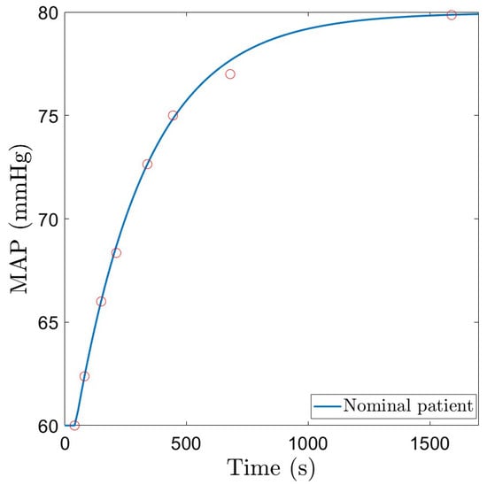
Figure 1.
Nominal patient model response to a constant infusion of Norepinephrine.

Table 1.
Nominal patient parameters and possible variation range.
The simplified mathematical model in (6) represents a generalized adult patient model, as it was developed based on the assumptions in [12,13,14,35]. The nominal patient model corresponds to an adult septic shock patient, as the parameters of the model have been estimated using clinical data from [15]. Different patients and different conditions would lead to different values of the model parameters. As such, in Table 1, the model parameters are varied to correspond to different types of adult patients.
The nominal patient model in Table 1 is further utilized in designing the dedicated control strategies. To account for patient variability, a robustness test is also performed. This is simulated via parameter variations of the model in (6), in the range indicated in Table 1 (variations in the gain K are included). The MAP signals corresponding to these patients as a function of a step change in the administered drug NOR(s) are given in Figure 2.
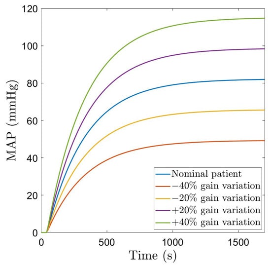
Figure 2.
Patient variability: MAP as a function of a step change in the administered drug NOR.
Remark 1.
The model developed in this paper and given in (6) could be further refined using synthetic data created based on two existing patient simulators [7,8], as well as using clinical data from the VitalDB database [36].
Two different control strategies have been designed, tested, and validated to control MAP, by manipulating the NOR drug dosage. In all cases, the model in (6) has been used to design the controllers. In contrast to existing control strategies that focus on the use of the simple PID controller, advanced control strategies are proposed in this paper to enhance the closed loop performance and robustness.
3. The Predictive Control Strategy
In this section, some theoretical aspects regarding the implementation of an EPSAC controller [29] will be given. The reader is referred to [37] for more details. The block diagram that depicts the EPSAC control strategy is given in Figure 3 [37].
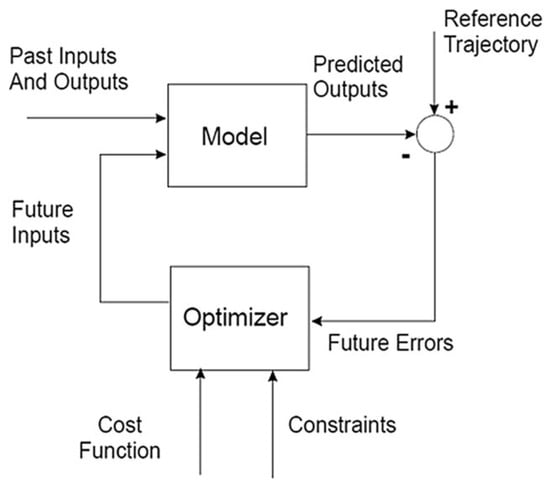
Figure 3.
EPSAC control scheme [37].
The measurable process output can be defined as follows:
where denotes the model output and denotes the real disturbance of the process, which is a non-measurable signal, including all the effects that may appear in the measured output that are not caused by the process input via . The disturbance is considered to have a stochastic character with non-zero average value that is modeled as colored noise:
where is white noise, is the backward shift operator, and is a filter that models the disturbance.
The signal from (9) can be defined as a generic dynamic model that depends on previous inputs and possibly also on previous outputs:
with a known function that implements the recurrent relation linking the model output to the input signal.
A fundamental part of a predictive controller is to calculate the predicted process output based on the postulated values of the input together with the measurements available at each sample time. At each current moment t, the process output will be predicted over a time horizon , where is the prediction horizon. From the generic process model, the following equation is obtained:
The prediction of depends on and . The prediction of is performed by recursion of the process model in (11) [37]. The current value of the disturbance is computed using the measured process output and the model output as . The prediction in the EPSAC methodology is based on filtering techniques. As such, the filtered disturbance signal is computed:
Based on (10) and (13), the signal is in fact white noise . Since white noise is uncorrelated, its best prediction is its mean value; thus, , with . Then, the prediction of the disturbance can be easily computed using
The recursive relation computed based on (14) allows for the computation of the predicted values for the disturbance , for , since .
In the EPSAC methodology, the objective is to find the control vector with , which minimizes a cost function defined as follows:
where and , for . The signal is the reference trajectory, beginning at and describing over the entire prediction horizon how the process output should evolve. Several other parameters in (15) are defined as follows: is the control horizon and is a weighting factor. The default values, considered also in this paper, are and .
For linear models, as in the case of the current paper, the predicted future response is viewed as the combined result of two components: , which represents the evolution of the system based on the process model, and , which accounts for the effect of future (postulated) control actions [37]:
The component can be easily computed using the procedure previously described, taking . The component represents the effect of a succession of unit step inputs with amplitude at time t, resulting in contributions to the process output k sampling periods later, to the process output sampling periods later, etc. The effect of all these contributions can be mathematically expressed as follows:
where the parameters , , …, … represent the coefficients of the unit step response of the system. For linear systems, these parameters can be easily determined by applying a unit step input to the process model. The signal computed over the prediction horizon can be written based on (17):
where is the minimum prediction horizon, with in most of the cases [37].
The cost function firstly introduced in (15) is now defined in a matrix form as
where is a vector that defines the reference trajectory. The objective is to maintain a constant setpoint throughout the entire simulation period, regardless of any disturbances. Using the identity matrix and minimizing (21) with respect to the input signal U, the optimal solution is obtained:
For the purpose of calculating the real control input , only the first element is necessary due to the principle of ‘receding horizon’, in which the steps presented in this section are recalculated at each sampling instant using the new measured information [37]. Further details regarding a more extensive explanation of the EPSAC algorithm are included in [37].
4. The Fractional Order Control Strategy
Fractional order controllers are generalizations of the integer order ones [38]. To control MAP, a fractional order PI (FO-PI) controller is designed, having a transfer function given as follows:
where and are the proportional and integral gains, and is the fractional order. The supplementary tuning parameter , as indicated in (23), allows for an increased flexibility and robustness of the closed loop system. As indicated in (23), there are three parameters to tune. Hence, three frequency domain performance specifications are imposed to determine the parameters. These performance criteria refer to a certain gain crossover frequency , a specific phase margin PM, and robustness to gain variations.
The gain crossover frequency specification implies that the closed loop system will exhibit a specific settling time. Mathematically, this specification is expressed using the magnitude of the open loop transfer function :
The second performance specification refers to the phase margin, which indirectly implies that the closed loop system will exhibit a specific overshoot. Mathematically, this specification is expressed using the phase of the open loop transfer function at the gain crossover frequency:
The third performance specification refers to the robustness to gain variations, a criterion that was imposed to account for patient variability. This implies that the PM remains constant despite gain variations and is mathematically represented as follows:
The equations in (24)–(26) require the frequency response of the controller and process, along with the corresponding magnitude, phase, and derivative of the phase with respect to the gain crossover frequency . They are computed hereafter.
The frequency response of the controller in (23) is obtained as follows:
yielding the following magnitude, phase, and derivative of the phase to be replaced in (24)–(26):
The magnitude of the controller frequency response in (28) and of the process in (31) are now replaced into (24), resulting in
Finally, the derivatives of the process and controller phases from (30) and (33) are replaced into (26), resulting in
Note that in (34)–(36), the only unknown parameters are those of the FO-PI controller. The last two Equations (35) and (36) contain two unknown parameters, namely and . This system of two nonlinear equations with two unknown parameters can be solved using graphical approaches [39] to determine first and . The algorithm assumes that the integral gain is computed as a function of the fractional order based on (35). The results are stored in a vector, denoted as . At the same time, the integral gain is again computed as a function of the fractional order using (36), with results stored in a vector denoted as . The two vectors and are plotted as a function of and the solution is obtained at the intersection point. The pseudo-code is described as follows:
| For , |
| Solve (35) and determine . Store values in vector . |
| Solve (36) and determine . Store values in vector . |
| Plot and as a function of and determine intersection point: and . |
The values estimated at the intersection point ( and ) correspond to the final values for and that meet both the phase margin and the robustness criteria in (35) and (36). Once the integral gain and the fractional order have been estimated, the proportional gain is computed using (34).
To design the FO-PI controller for the MAP, specific values for the and PM need to be selected and used in the design Equations (34)–(36). Several choices for the phase margin and gain crossover frequency are possible. In the case of MAP, a small overshoot implies a significantly large settling time, whereas a smaller settling time comes with the drawback of a larger overshoot. A compromise was made between the duration of the settling time and the overshoot, with the final choice for the performance specifications being = 0.009 rad/s and PM = 50o, along with the robustness to gain variations condition. The selected values for and are now replaced into (35) and (36). The algorithm described above is used to estimate the integral gain as a function of and to determine the vectors and . Figure 4 shows the two vectors as a function of the fractional order . The intersection point yields and . Replacing these values into (34) results in . The final transfer function of the resulting FO-PI controller is then given as
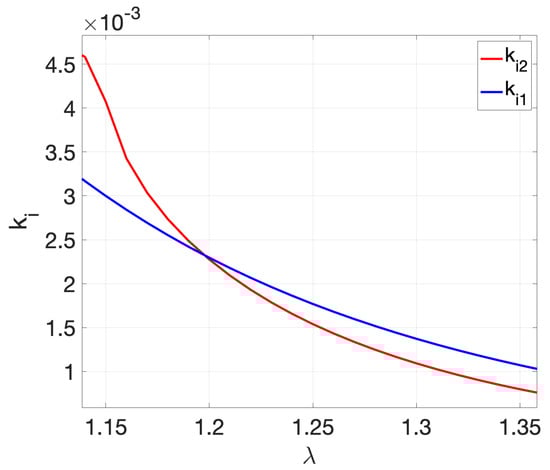
Figure 4.
Graphical solution to determine and .
To implement the fractional order controller, a continuous-time approximation is produced using the Oustaloup Recursive Approximation method [40]. The approximation is valid in the range of (0.0001–0.01) rad/s, which includes the gain crossover frequency. The order of approximation is , resulting in a higher-order transfer function with poles and zeros. The continuous-time transfer function is further approximated with a discrete-time transfer function using the Zero-Order Hold method and a sampling period equal to 20 s. The Bode diagram of the original FO-PI controller in (37) and the discrete-time approximation is given in Figure 5 and clearly shows that the discrete-time approximation is accurate.
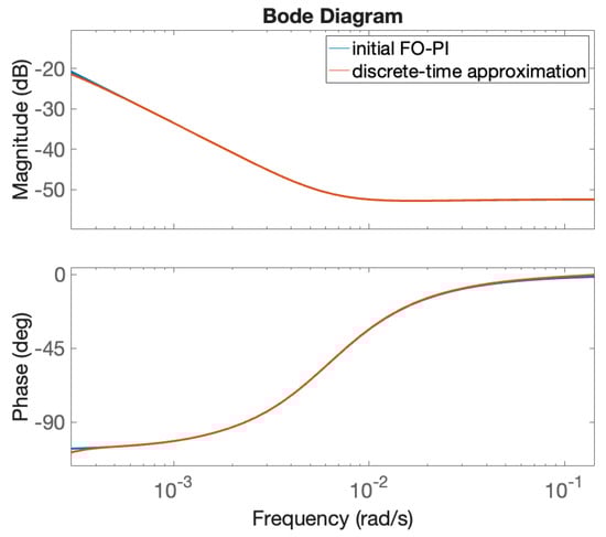
Figure 5.
Frequency response of the original FO-PI controller in (37) and its discrete-time approximation.
The closed loop simulation results are included in the following section.
5. Closed Loop Simulation Results
Different case studies have been considered to test the advantages and limitations of the two control strategies. Both reference tracking and disturbances rejection case studies were considered. The closed loop results were evaluated for a nominal patient, as well as for various gain variations. This type of parameter variation has been chosen since the fractional order PI controller has been specifically designed to be robust to such variations.
In the closed loop simulation results included in this section, the nominal patient model corresponds to parameter values taken as , , and . Gain variations of are also considered to test the robustness of the two control strategies, with K taking values such as 470, 940, 1410, and 1645. In both cases, the initial value for the MAP is considered to be 60 mmHg, and it is driven using the two control strategies to a new setpoint equal to 80 mmHg. The initial dose of administered Norepinephrine infusion starts at a constant value, suited for each patient. The controller indicated in (37) is used to evaluate the closed loop performance of the fractional order control algorithm. For the EPSAC controller, a first-order Padé approximation has been used for the time delay of the nominal patient. This approximation does not affect the overall closed loop results and solely results in a nonminimum phase effect visible when step changes in the reference signal are considered. To implement the EPSAC controller, a sampling period of 10 s was considered, the minimum and maximum prediction horizons were taken as and , as a compromise between robustness and faster settling time.
The closed loop simulation results considering the fractional order controller and the nominal patient, as well as gain variations are given in Figure 6. The corresponding NOR signal is indicated in Figure 7. For the nominal patient, an overshoot of and a settling time of 675 s are obtained. For and gain variations, the overshoot remains quasi constant, ranging from to . This demonstrates the robustness of the designed FO-PI controller to gain variations. The settling time ranges from 570 s to 900 s. The NOR drug rate remains within the usual clinically accepted values.
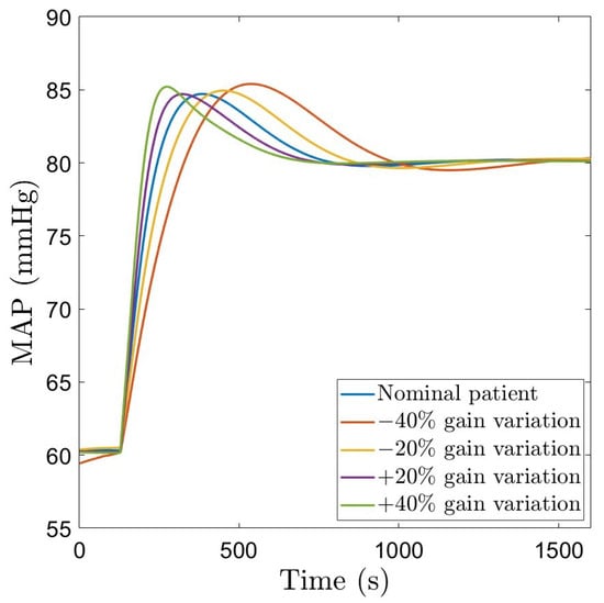
Figure 6.
Closed loop simulation results using a robust FO-PI controller.
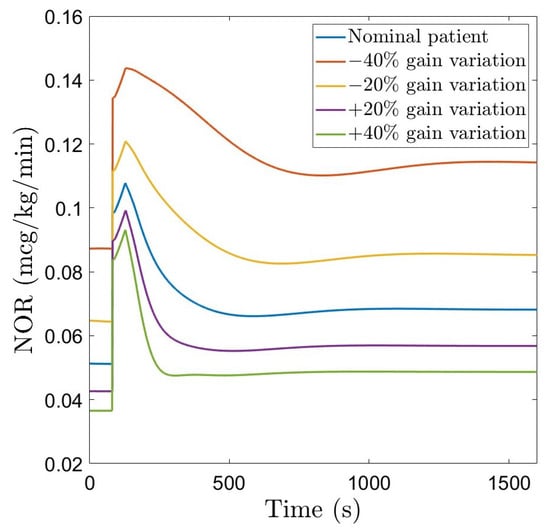
Figure 7.
NOR drug rate using the robust FO-PI controller.
The closed loop simulation results with the EPSAC controller for the nominal patient, as well as gain variations are given in Figure 8, with the corresponding NOR signal given in Figure 9. For the nominal patient, as well as for gain variations, the overshoot remains at , a clear advantage of this approach compared to the fractional order PI controller. The settling time for the nominal patient is approximately 600 s, smaller than that obtained with the fractional order controller. In terms of gain variations, the system output remains without overshoot, with a larger variation of the settling time (500–950 s), compared to the fractional order controller. The NOR infusion rate remains within the limits.
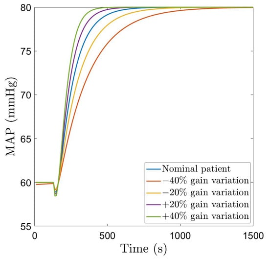
Figure 8.
Closed loop simulation results using robust EPSAC.
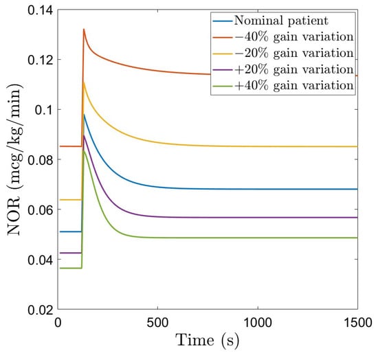
Figure 9.
NOR drug rate using the robust EPSAC.
The manipulated variable (dose of Norepinephrine) indicated in Figure 7 and Figure 9 has a larger amplitude spike at the beginning, when the controller is trying to reach the setpoint chosen by the user, and afterwards, it stabilizes at a constant value. Nevertheless, throughout the entire simulation, the NOR dose rate remains within realistic values.
A step disturbance causing a drop of 5 mmHg in MAP is considered to test the ability of the controllers to reject disturbances. Figure 10a and Figure 11a show the closed loop simulation results obtained with the FO-PI and the EPSAC controller, respectively. The FO-PI controller manages to reject the disturbance in approximately 500 s, with some slight oscillations. The EPSAC controller, on the other hand, is more efficient in resolving the disturbance with a rejection time of approximately 400 s and no oscillations. The drug doses in both cases are kept within normal limits (Figure 10b and Figure 11b). A pseudo-random binary sequence (PRBS)-type signal is also implemented as a disturbance. The PRBS signal was created using the Matlab function idinput with a magnitude of 0.5 mmHg. This kind of disturbance impacts MAP with deviations between 80.5 mmHg and 79.3 mmHg from the standard 80 mmHg, which we imposed as a setpoint for the two advanced controllers. In a similar manner, the input presents a deviation of ±0.003 μg/kg/min from the usual induced dose. For the fractional order controller, this disturbance was introduced at the second 900 and lasts for approximately 1100 s, while for the EPSAC controller, this disturbance starts later in the simulation, at the second 1000, and lasts for the same amount of time. The closed loop simulation results are included in Figure 10c and Figure 11c, with the corresponding drug inputs given in Figure 10d and Figure 11d.
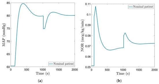
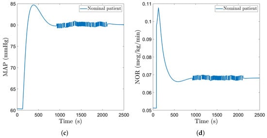
Figure 10.
Disturbances–fractional order controller: (a) MAP of nominal patient with step disturbance. (b) Administered NOR for nominal patient with step disturbance. (c) MAP of nominal patient with PRBS disturbance. (d) Administered NOR for nominal patient with PRBS disturbance.
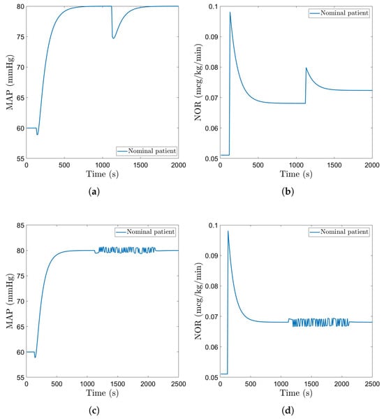
Figure 11.
Disturbances–EPSAC: (a) MAP of nominal patient with step disturbance. (b) Administered NOR for nominal patient with step disturbance. (c) MAP of nominal patient with PRBS disturbance. (d) Administered NOR for nominal patient with PRBS disturbance.
6. Comparative Analysis, Advantages, and Limitations
The two control strategies are evaluated comparatively in this section. First of all, in terms of reference tracking, the EPSAC controller achieves better overshoot compared to the FO-PI controller. The settling time of the EPSAC controller ranges between 500 and 950 s, slightly poorer compared to the FO-PI controller with a settling time between 570 and 900 s. Both the EPSAC and FO-PI controllers are robust to the gain variations (maintaining a constant overshoot despite the significant gain variations of .
A simple PI controller is also designed for comparative purposes. To the best of the author’s knowledge, only PID-type controllers have been so far reported as a closed loop control strategy for MAP regulation using NOR [1,16,17,18,19]. No details regarding the actual tuning of this PID controller are included. Hence, the PI controller is designed similarly to the FO-PI, for a fair comparison. The transfer function of the PI controller is similar to (23), with . The same gain crossover frequency rad/s and phase margin are used to tune the parameters of the PI controller. Since the PI controller has only two tuning parameters, the proportional and integral gain, only two tuning equations are necessary: the magnitude equation in (34) and (35). The integral gain is computed first using the (35), where now , yielding . The proportional gain is computed next using (34), with , resulting in . The closed loop simulation results using this PI controller are included in Figure 12.
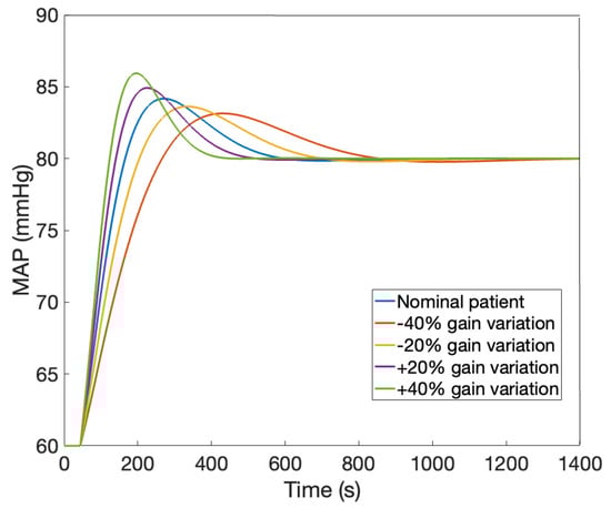
Figure 12.
Closed loop simulation results using a PI controller.
Table 2 presents a quantitative comparison between the closed loop results obtained with the EPSAC, the FO-PI, and the PI controller, in terms of reference tracking. The results are compared in terms of overshoot and settling time, for both the nominal patient and gain variations.
Table 2.
Comparative results for reference tracking.
Based on the results in Table 2, the EPSAC controller is a better choice if the overshoot is more important. In terms of settling time, the traditional PI controller achieves a faster response time compared to the EPSAC and the FO-PI. The drawback of this PI controller is the reduced robustness compared to the EPSAC or the FO-PI controller. In both of the proposed control algorithms, the overshoot remains constant despite the significant gain variations, whereas in the case of the PI controller, the overshoot varies between and nearly double .
In what follows, the two proposed control methods are evaluated also in terms of required NOR drug rate and disturbance rejection. Regarding the control signal, the NOR drug rate, the two methods are similar. They both present a slightly increased amplitude spike when fluctuations in the MAP appear, with the fractional order proportional integral controller reaching a higher value. Despite that, the FO-PI also seems to present a more gradual decrease in the command value than the EPSAC. Otherwise, the manipulated variable presents a similar behavior in both cases.
For step disturbance rejection, the two controllers require a similar control effort (increase in the administered drug). The EPSAC controller has a slightly better response time (approximately 400 s) compared to that achieved by the FO-PI (approximately 500 s). The disturbance rejection time of the FO-PI controller could be further reduced by using a more complex fractional order controller that includes the derivative component, as well.
A comparison of the disturbance rejection scenario when the PRBS-type disturbance signal is considered shows a similar control effort. A comparison of the closed loop responses in terms of the mean square error (MSE) leads to the following results: the MSE of the EPSAC is equal to 0.2403 and the MSE of the FO-PI is equal to 0.2665. These results show once more that the EPSAC has a slightly better response than the FO-PI. A larger amplitude of the PRBS signal would lead to larger values of the MSE, but the EPSAC controller would still prevail over the FO-PI.
Several limitations of the proposed control algorithms need to be mentioned here. First of all, the design and implementation of the predictive controller requires multiple resources involving matrix computations and optimizations. On the other hand, the implementation of the fractional order controller firstly undergoes an approximation using standard techniques such as the Oustaloup Recursive Approximation method [40] to produce a continuous-time approximation, as indicated in Section 4. Then, a discrete-time approximation is performed using standard discretization techniques, which finally leads to a recurrent relation for the control signal. For the case study considered in this manuscript, the discrete-time approximation of the FO-PI controller in (37) is obtained as detailed in Section 4:
with the computed drug rate and the error signal at every sample. Here, refers to the MAP setpoint or reference value and is the measured MAP signal. The polynomials are obtained as follows: and , with the backward shift operator. For a practical implementation, the discrete-time transfer function in (38) leads to a recurrent relation of the control signal (NOR drug rate) computed based on (38):
According to (39), the computation of the control signal is based on simple mathematical operations such as scalar summation and multiplication. The FO-PI controller requires a lower computational power with a better run time of the algorithm overall. In both cases, the control algorithm can be implemented on a computer, connected to the MAP monitor in order to pass the measured patient signal to the control algorithm.
Secondly, the tuning of the FO-PI controller is not trivial. Several combinations of and PM have been considered and tested for designing the fractional order PI controller. A smaller overshoot can be obtained by imposing a larger phase margin PM and a smaller gain crossover frequency . However, this would have led to an increased settling time. This represents an important limitation of the fractional order PI controller. The values selected and mentioned in this manuscript = 0.009 rad/s and were considered to be optimal. To diminish the settling time and reduce the overshoot, a more complex fractional order controller could be designed by altering the FO-PI controller to include a derivative component, as well.
Lastly, the model developed in this manuscript is based on a limited dataset of clinical data. The results are thus preliminary but demonstrate that advanced control strategies could be successfully used in a automatic Norepinephrine drug dosing to maintain the MAP signal within a safe range. Further research includes the use of the very recent patient simulators in [7,8] to generate artificial data, as well as clinical data available in the VitalDB database [36] to further refine and validate the simplified model developed in this manuscript. The existing PK-PD models, used as a starting point in the development of the simplified model in this manuscript, are valid for a specific class of patients, under septic shock. A universally applicable patient model is the scope of further research, which implies access to a larger dataset of clinical data.
7. Conclusions
The current paper aimed to develop a mathematical model which describes the effect that Norepinephrine infusion has on mean arterial pressure, one that is suitable for designing controllers. A subsequent aim was to implement, test, compare, and analyze advanced control strategies. These were designed in order to shorten the settling time and handle problems such as setpoint changes, patient variability, and disturbances.
The scarcity of real clinical data and established PK-PD relationships presents a major hurdle when developing a mathematical model for controller design. That being said, the model derived for this paper draws from available information on the aforementioned, and it is therefore limited to a certain type of patient.
Regarding automated drug administration, an important part of implementing any type of controller is having a good understanding of both the manipulated and controlled variables and maintaining them within the limits recommended by medical professionals. Consequently, all of the principles implemented in this paper respect these arguments. The EPSAC and FO-PI methods are therefore suitable for further studies regarding the automatic control of MAP using NOR infusion.
The results in this paper are preliminary, based on a reduced clinical dataset. Information from available databases, such as the VitalDB [36], could be further used to develop a more accurate model and a better design of the controllers. Additionally, a model for cardiac output and related drugs to obtain a multivariable hemodynamic system similar to (1) might enhance the perspectives upon the hemodynamic system and automatic regulation of hemodynamic variables.
Author Contributions
Conceptualization, T.M.P. and C.I.M.; methodology, T.M.P.; software, T.M.P. and I.R.B.; validation, T.M.P., N.E.B. and C.I.M.; formal analysis, T.M.P. and N.E.B.; investigation, A.M.T. and A.C.M.; resources, T.M.P. and I.R.B.; data curation, A.M.T. and A.C.M.; writing—original draft preparation, T.M.P. and N.E.B.; writing—review and editing, C.I.M. and I.R.B.; visualization, T.M.P., A.M.T. and A.C.M.; supervision, C.I.M.; project administration, C.I.M.; funding acquisition, C.I.M. All authors have read and agreed to the published version of the manuscript.
Funding
This work was supported in part by a grant of the Romanian Ministry of Research, Innovation and Digitization, PNRR-III-C9-2022–I8, grant number 760068/23.05.2023. I. R. Birs acknowledges the support of Flanders Research Foundation, Postdoc grant 1203224N, 2023–2026. I.R.Birs was financed by a grant of the Ministry of Research, Innovation and Digitization, CNCS-UEFISCDI, project number PN-IV-P2-2.1-TE-2023-0831.
Institutional Review Board Statement
Not applicable; all data was generated using simulations and mathematical models.
Informed Consent Statement
Not applicable; all data was generated using simulations and mathematical models.
Data Availability Statement
All data presented in this research can be easily generated using the provided mathematical models and controllers.
Conflicts of Interest
The authors declare no conflicts of interest.
References
- Joosten, A.; Chirnoaga, D.; Van der Linden, P.; Barvais, L.; Alexander, B.; Duranteau, J.; Vincent, J.L.; Cannesson, M.; Rinehart, J. Automated closed-loop versus manually controlled norepinephrine infusion in patients undergoing intermediate- to high-risk abdominal surgery: A randomised controlled trial. Br. J. Anaesth. 2021, 126, 210–218. [Google Scholar] [CrossRef]
- Rao, R.; Aufderheide, B.; Bequette, B. Experimental studies on multiple-model predictive control for automated regulation of hemodynamic variables. IEEE Trans. Biomed. Eng. 2003, 50, 277–288. [Google Scholar] [CrossRef]
- Lee, S.; Park, D.; Ju, J.W.; Bae, J.; Cho, Y.J.; Nam, K.; Jeon, Y. Relationship between intraoperative dopamine infusion and postoperative acute kidney injury in patients undergoing open abdominal aorta aneurysm repair. BMC Anesthesiol. 2022, 22, 82. [Google Scholar] [CrossRef] [PubMed]
- Campese, V.M.; Lakdawala, R.S. Chapter 53—The Challenges of Blood Pressure Control in Dialysis Patients. In Handbook of Dialysis Therapy, 5th ed.; Nissenson, A.R., Fine, R.N., Eds.; Elsevier: Amsterdam, The Netherlands, 2017; pp. 603–626.e2. [Google Scholar] [CrossRef]
- Sniecinski, R.M.; Wright, S.; Levy, J.H. Chapter 3—Cardiovascular Pharmacology. In Cardiothoracic Critical Care; Sidebotham, D., Mckee, A., Gillham, M., Levy, J.H., Eds.; Butterworth-Heinemann: Philadelphia, PA, USA, 2007; pp. 33–52. [Google Scholar] [CrossRef]
- Pimenta, E.; Calhoun, D.A.; Oparil, S. CHAPTER 28—Hypertensive Emergencies. In Cardiac Intensive Care, 2nd ed.; Jeremias, A., Brown, D.L., Eds.; W.B. Saunders: Philadelphia, PA, USA, 2010; pp. 355–367. [Google Scholar] [CrossRef]
- Aubouin–Pairault, B.; Dang, T.; Fiacchini, M. PAS: A Python Anesthesia Simulator for drug control. J. Open Source Softw. 2023, 8, 5480. [Google Scholar] [CrossRef]
- Hosseinirad, S.; Merlo, M.; Trovò, F.; Tognoli, E.; Metelli, A.M.; Dumont, G.A. AReS: A patient simulator to facilitate testing of automated anesthesia. Comput. Methods Programs Biomed. 2025, 269, 108901. [Google Scholar] [CrossRef]
- van Limmen, J.; Iturriagagoitia, X.; Verougstraete, M.; Wyffels, P.; Berrevoet, F.; de Carvalho, L.A.; Hert, S.D.; Baerdemaeker, L.D. Effect of norepinephrine infusion on hepatic blood flow and its interaction with somatostatin: An observational cohort study. BMC Anesth. 2022, 22, 202. [Google Scholar] [CrossRef]
- Backer, D.D.; Pinsky, M. Norepinephrine improves cardiac function during septic shock, but why? Br. J. Anaesth. 2018, 120, 421–424. [Google Scholar] [CrossRef]
- Hamzaoui, O.; Jozwiak, M.; Geffriaud, T.; Sztrymf, B.; Prat, D.; Jacobs, F.; Monnet, X.; Trouiller, P.; Richard, C.; Teboul, J. Norepinephrine exerts an inotropic effect during the early phase of human septic shock. Br. J. Anaesth. 2018, 120, 517–524. [Google Scholar] [CrossRef]
- Beloeil, H.; Mazoit, J.X.; Benhamou, D.; Duranteau, J. Norepinephrine kinetics and dynamics in septic shock and trauma patients. Br. J. Anaesth. 2005, 95, 782–788. [Google Scholar] [CrossRef] [PubMed]
- Oualha, M.; Tréluyer, J.M.; Lesage, F.; de Saint Blanquat, L.; Dupic, L.; Hubert, P.; Spreux-Varoquaux, O.; Urien, S. Population pharmacokinetics and haemodynamic effects of norepinephrine in hypotensive critically ill children. Br. J. Clin. Pharmacol. 2014, 78, 886–897. [Google Scholar] [CrossRef]
- Joachim, J.; Cartailler, J.; Vallee, F.; Lefevre, T.; Callebert, J.; Gayat, E.; Lavielle, M. Design of a pharmacokinetic/pharmacodynamic model for administration of low dose peripheral norepinephrine during general anaesthesia. Br. J. Clin. Pharmacol. 2024, 90, 2861–2869. [Google Scholar] [CrossRef]
- Tang, Y.; Brown, S.; Sorensen, J.; Harley, J. Physiology-Informed Real-Time Mean Arterial Blood Pressure Learning and Prediction for Septic Patients Receiving Norepinephrine. IEEE Trans. Biomed. Eng. 2021, 68, 181–191. [Google Scholar] [CrossRef]
- Joosten, A.; Alexander, B.; Duranteau, J.; Taccone, F.S.; Creteur, J.; Vincent, J.L.; Cannesson, M.; Rinehart, J. Feasibility of closed-loop titration of norepinephrine infusion in patients undergoing moderate- and high-risk surgery. Br. J. Anaesth. 2019, 123, 430–438. [Google Scholar] [CrossRef]
- Desebbe, O.; Rinehart, J.; der Linden, P.V.; Cannesson, M.; Delannoy, B.; Vigneron, M.; Curtil, A.; Hautin, E.; Vincent, J.; Duranteau, J.; et al. Control of Postoperative Hypotension Using a Closed-Loop System for Norepinephrine Infusion in Patients After Cardiac Surgery: A Randomized Trial. Anesth. Analg. 2022, 134, 964–973. [Google Scholar] [CrossRef]
- Joosten, A.; Rinehart, J.; Cannesson, M.; Coeckelenbergh, S.; Pochard, J.; Vicaut, E.; Duranteau, J. Control of mean arterial pressure using a closed-loop system for norepinephrine infusion in severe brain injury patients: The COMAT randomized controlled trial. J. Clin. Monit. Comput. 2024, 38, 25–30. [Google Scholar] [CrossRef] [PubMed]
- Coeckelenbergh, S.; Soucy-Proulx, M.; der Linden, P.V.; Clanet, M.; Rinehart, J.; Cannesson, M.; Duranteau, J.; Joosten, A. Tight control of mean arterial pressure using a closed loop system for norepinephrine infusion after high-risk abdominal surgery: A randomized controlled trial. J. Clin. Monit. Comput. 2024, 38, 19–24. [Google Scholar] [CrossRef]
- Coronel-Escamilla, A.; Gomez-Aguilar, J.; Stamova, I.; Santamaria, F. Fractional order controllers increase the robustness of closed-loop deep brain stimulation systems. Chaos Solitons Fractals 2020, 140, 110149. [Google Scholar] [CrossRef] [PubMed]
- Alavi, M.B.; Tabatabaei, M. Control of depth of anaesthesia using fractional-order adaptive high-gain controller. IET Syst. Biol. 2019, 13, 36–42. [Google Scholar] [CrossRef] [PubMed]
- Hegedus, E.; Ghita, M.; Birs, I.R.; Copot, D.; Muresan, C.I. Robustness analysis of a fractional order control system for the hemodynamic variables in anesthetized patients. In Proceedings of the 2023 European Control Conference (ECC), Bucharest, Romania, 13–16 June 2023; pp. 1–6. [Google Scholar] [CrossRef]
- Badau, N.E.; Popescu, T.M.; Mihai, M.D.; Birs, I.R.; Muresan, C.I. A Robust Fractional-Order Controller for Biomedical Applications. Fractal Fract. 2025, 9, 597. [Google Scholar] [CrossRef]
- Muresan, C.I.; Mihai, M.D.; Hegedus, E.; Badau, N.; Popescu, T.; Birs, I.R. Robust Fractional Order Control of a Multivariable Hemodynamic System. In Proceedings of the 2025 33rd Mediterranean Conference on Control and Automation (MED), Tangier, Morocco, 10–13 June 2025; pp. 678–683. [Google Scholar] [CrossRef]
- Ionescu, C.M.; Copot, D.; De Keyser, R. Anesthesiologist in the Loop and Predictive Algorithm to Maintain Hypnosis While Mimicking Surgical Disturbance. IFAC-PapersOnLine 2017, 50, 15080–15085. [Google Scholar] [CrossRef]
- Ionescu, C.M.; De Keyser, R.; Copot, D.; Yumuk, E.; Birs, I.R.; Hegedus, E.; Muresan, C.I.; Neckebroek, M. Minimizing Epistemic Uncertainty for Predictive Control of General Anesthesia. IFAC-PapersOnLine 2024, 58, 490–495. [Google Scholar] [CrossRef]
- Aubouin–Pairault, B.; Fiacchini, M.; Dang, T. PID and Model Predictive Control Approach for Drug Dosage in Anesthesia During Induction: A Comparative Study. IFAC-PapersOnLine 2024, 58, 210–215. [Google Scholar] [CrossRef]
- Ionescu, C.M.; Neckebroek, M.; Ghita, M.; Copot, D. An Open Source Patient Simulator for Design and Evaluation of Computer Based Multiple Drug Dosing Control for Anesthetic and Hemodynamic Variables. IEEE Access 2021, 9, 8680–8694. [Google Scholar] [CrossRef]
- Maxim, A.; Copot, D. Closed-loop control of anesthesia and hemodynamic system: A Model Predictive Control approach. IFAC-PapersOnLine 2021, 54, 37–42. [Google Scholar] [CrossRef]
- Farbakhsh, H.; Yumuk, E.; Othman, G.B.; Keyser, R.D.; Copot, D.; Birs, I.; Ionescu, C.M. Model predictive control of hemodynamics during intravenous general anesthesia. In Proceedings of the 2023 27th International Conference on System Theory, Control and Computing (ICSTCC), Timisoara, Romania, 11–13 October 2023; pp. 362–367. [Google Scholar] [CrossRef]
- Popescu, T.; Birs, I.R.; Othman, G.B.; Yumuk, E.; Mihai, M.; Hegedus, E.; Copot, D.; De Keyser, R.; Ionescu, C.M.; Muresan, C.I. Uncertainty and its Effect on Optimal Multidrug Control of Hemodynamic Variables. In Proceedings of the 2024 American Control Conference (ACC), Toronto, ON, Canada, 8–9 July 2024; pp. 3891–3896. [Google Scholar] [CrossRef]
- Ahmadpour, M.R.; Ghadiri, H.; Hajian, S.R. Model predictive control optimisation using the metaheuristic optimisation for blood pressure control. IET Syst. Biol. 2021, 15, 41–52. [Google Scholar] [CrossRef]
- Adeodu, O.; Gee, M.; Mahmoudi, B.; Vadigepalli, R.; Kothare, M. Nonlinear Model Predictive Control of Vagal Nerve Stimulation to regulate hemodynamic variables. IFAC-PapersOnLine 2023, 56, 6525–6530. [Google Scholar] [CrossRef]
- Neckebroek, M.; Ionescu, C.; van Amsterdam, K.; Smet, T.D.; Baets, P.D.; Decruyenaere, J.; Keyser, R.D.; Struys, M. A comparison of propofol-to-BIS post-operative intensive care sedation by means of target controlled infusion, Bayesian-based and predictive control methods: An observational, open-label pilot study. J. Clin. Monit. Comput. 2019, 33, 675–686. [Google Scholar] [CrossRef]
- He, H.W.; Liu, W.L.; Zhou, X.; Long, Y.; Liu, D.W. Effect of mean arterial pressure change by norepinephrine on peripheral perfusion index in septic shock patients after early resuscitation. Chin. Med. J. 2020, 133, 2146–2152. [Google Scholar] [CrossRef] [PubMed]
- Lee, H.; Park, Y.; Yoon, S.e.a. VitalDB, a high-fidelity multi-parameter vital signs database in surgical patients. Sci. Data 2022, 9, 279. [Google Scholar] [CrossRef]
- De Keyser, R. Model based predictive control for linear systems. In UNESCO Encyclopaedia of Life Support Systems; UNESCO: Paris, France, 2003. [Google Scholar]
- Tejado, I.; Vinagre, B.M.; Traver, J.E.; Prieto-Arranz, J.; Nuevo-Gallardo, C. Back to Basics: Meaning of the Parameters of Fractional Order PID Controllers. Mathematics 2019, 7, 530. [Google Scholar] [CrossRef]
- Birs, I.; Muresan, C.; Nascu, I.; Ionescu, C. A Survey of Recent Advances in Fractional Order Control for Time Delay Systems. IEEE Access 2019, 7, 30951–30965. [Google Scholar] [CrossRef]
- Reddy, A.; Reddy, G. Novel applications of oustaloup recursive approximation and modified oustaloup recursive approximation methods in linear fractional order control design. Int. J. Dyn. Control 2024, 12, 2236–2246. [Google Scholar] [CrossRef]
Disclaimer/Publisher’s Note: The statements, opinions and data contained in all publications are solely those of the individual author(s) and contributor(s) and not of MDPI and/or the editor(s). MDPI and/or the editor(s) disclaim responsibility for any injury to people or property resulting from any ideas, methods, instructions or products referred to in the content. |
© 2025 by the authors. Licensee MDPI, Basel, Switzerland. This article is an open access article distributed under the terms and conditions of the Creative Commons Attribution (CC BY) license (https://creativecommons.org/licenses/by/4.0/).