Abstract
Exoskeleton-assisted bodyweight support training (BWST) has demonstrated enhanced neurorehabilitation outcomes in which joint motion prediction serves as the critical foundation for adaptive human–machine interactive control. However, joint angle prediction under dynamic unloading conditions remains unexplored. This study introduces an adaptive wavelet-denoising fusion (AWDF) model to predict lower-limb joint angles during BWST. Utilizing a custom human-tracking bodyweight support system, time series data of surface electromyography (sEMG), and inertial measurement unit (IMU) from ten adults were collected across graded bodyweight support levels (BWSLs) ranging from 0% to 40%. Systematic comparative experiments evaluated joint angle prediction performance among five models: the sEMG-based model, kinematic fusion model, wavelet-enhanced fusion model, late fusion model, and the proposed AWDF model, tested across prediction time horizons of 30–150 ms and BWSL gradients. Experimental results demonstrate that increasing BWSLs prolonged gait cycle duration and modified muscle activation patterns, with a concomitant decrease in the fractal dimension of sEMG signals. Extended prediction time degraded joint angle estimation accuracy, with 90 ms identified as the optimal tradeoff between system latency and prediction advancement. Crucially, this study reveals an enhancement in prediction performance with increased BWSLs. The proposed AWDF model demonstrated robust cross-condition adaptability for hip and knee angle prediction, achieving average root mean square errors (RMSE) of 1.468° and 2.626°, Pearson correlation coefficients (CC) of 0.983 and 0.973, and adjusted R2 values of 0.992 and 0.986, respectively. This work establishes the first computational framework for BWSL-adaptive joint prediction, advancing human–machine interaction in exoskeleton-assisted neurorehabilitation.
1. Introduction
Bodyweight-supported training (BWST) is employed in neurological rehabilitation to facilitate gait training through partial weight unloading. This therapeutic approach reduces biomechanical loads for non-ambulatory patients while maintaining postural stability, thereby enabling safe completion of locomotor protocols and fall prevention during therapeutic sessions [1]. Clinical evidence confirms that exoskeleton-assisted BWST enhances locomotor recovery through adaptive BWSL modulation during repetitive gait training, particularly benefiting patients with stroke-induced or age-related mobility impairments [2,3].
Building on the therapeutic benefits of BWST, accurate motion intention recognition constitutes the foundation of active compliance control in lower-limb exoskeletons [4,5]. Human motion intention recognition encompasses discrete movement classification and continuous motion intention prediction. Current research prioritizes continuous motion intention prediction over discrete movement classification, particularly in exoskeleton control applications. However, current methodologies conflate estimation with prediction by employing synchronous joint angle estimation during motion execution, relying on biomechanical signals as post hoc data labels [6,7,8]; current research on lower-limb joint angle prediction remains limited. Importantly, continuous predictive algorithms outperform estimation-based approaches in compensating system latency and signal transmission delay inherent in human–robot interaction systems.
Surface electromyography (sEMG) captures the bioelectric potentials reflecting neuromuscular activation patterns associated with movement intention. In our previous studies, we have conducted research on sEMG-based gait pattern recognition and knee angle prediction [9,10]. Other researchers, such as Foroutannia et al. [11], developed a deep learning framework that decodes sEMG signals for hip joint position prediction and exoskeleton assistive torque calculation. Subsequent studies by Lu et al. [12] and Han et al. [13] further advanced the sEMG-based prediction using Conv-BiLSTM and ensemble XGBoost regression models, respectively. However, current research predominantly focuses on natural locomotion patterns (walking, running, stair ascent/descent), and prediction algorithms specifically adapted to BWST environments remain unexplored. The unique biomechanical context of BWST modulates lower-limb muscle strength, neuromuscular activation levels, coordination patterns, and movement characteristics. Liu et al. [14] demonstrated that different bodyweight support levels (BWSL), 0–40%, can lead to significant changes in the root mean square and other sEMG features of muscles. Consistent with these findings, Kristiansen et al. [15] and Bu et al. [16] quantified BWSL-induced changes in muscle activation levels and fiber dynamics during gait training. Das et al. [17] used Higuchi’s fractal dimension analysis to estimate fractal dimension of the sEMG signal, and implemented Detrended Fluctuation Analysis to examine the change in sEMG signals with varying weights. Critically, these neuromuscular adaptations may compromise the reliability of sEMG-based motion intention recognition. Nevertheless, the influence of BWSL variations on joint angle prediction accuracy has not been systematically investigated.
The selection of sEMG features under varying BWSLs critically influences motion intention prediction accuracy. Traditional methods primarily employ three categories of handcrafted features: time-domain, frequency-domain, and time-frequency domain. Lu et al. [12] systematically compared these features in regression models, while Song et al. [18] utilized RMS time features for joint angle prediction. Although these handcrafted features achieve moderate performance in controlled environments, their reliance on linear assumptions fails to address the non-stationary nature of sEMG signals and muscle synergy patterns under BWSL-induced neuromuscular adaptations. In contrast, deep learning approaches, such as CNN-based automatic feature extraction and unified spatiotemporal-frequency frameworks like Deep-STF [19,20], exhibit enhanced capability in modeling complex sEMG patterns. Despite the demonstrated superiority of model-based learning approaches for feature extraction in automatically capturing sEMG patterns, their performance becomes inherently constrained under varying BWSLs conditions. Specifically, sEMG signals are influenced by BWSL variations with changing muscle activation patterns. To address these challenges, adaptive signal processing techniques capable of capturing both temporal and spectral dynamics are imperative. This necessitates a paradigm shift toward methods that inherently accommodate the time-frequency variability of sEMG under dynamic unloading conditions.
Wavelet transform (WT) demonstrates unique advantages in addressing sEMG signal degradation through multi-resolution time-frequency analysis. Empirical studies validate the effectiveness of discrete wavelet transform (DWT) coefficients as discriminative features. Xi et al. [7] successfully estimated joint angles using wavelet coefficients, while Duan et al. [21] enhanced pattern recognition by selecting maximum absolute DWT coefficients. The robustness of this approach is further evidenced by Zafar et al. [22], who applied the DWT technique to extract features from the filtered sEMG signal for hand gesture recognition. These successes stem from WT’s ability to decompose non-stationary signals while preserving neuromuscular activation patterns through threshold-optimized coefficient selection. However, current implementations face critical limitations in BWST scenarios: fixed decomposition levels and static thresholds fail to adapt to BWSL-dependent SNR variations. Therefore, DWT coefficient features can be optimized with adaptive thresholds, effectively preserving neuromuscular activation features while mitigating BWSL-induced activation changes.
To address the challenges of predicting joint angles under dynamic BWSL conditions, this study proposes a novel adaptive wavelet-denoising fusion (AWDF) model for continuous joint angle prediction during BWST. To the best of our knowledge, this work represents the first systematic exploration of adaptive sEMG denoising and joint kinematics prediction tailored for BWST.
This applied contribution is designed to tackle the core hypothesis that (1) variations in BWSLs induce significant changes in the characteristics of muscle activation, which consequently affect joint angle prediction accuracy; (2) an optimal prediction time horizon exists that effectively balances the compensation for system latency against the degradation in prediction fidelity, and this horizon is feasible for real-time exoskeleton control; and (3) the proposed adaptive multi-feature fusion model will outperform baseline models in predicting hip and knee joint angles across all BWSLs.
Moving beyond these applied innovations, this work also ventures into a scientific exploration of the nonlinear dynamic properties of neuromuscular systems under BWST. We hypothesize that BWSL alterations not only change muscle activation intensity, but also fundamentally modulate the complexity and regularity of motor control strategies. To test this, we employ a multidimensional feature analysis—Higuchi’s fractal dimension [23,24], sample entropy [25], and root mean square [26]—to uncover the nuanced influences of BWSL on lower-limb muscle activities from complementary perspectives.
The rest of this paper is organized as follows: Section 2 introduces the architecture of the proposed AWDF prediction model and details the methodology for the feature analysis of sEMG signals. Section 3 describes the experimental platform and the detailed protocol designed for data collection. Section 4 presents the results, analyzing the impact of both BWSL and prediction time on model performance, as well as the trends observed in the sEMG feature analysis. Finally, the findings are thoroughly discussed in Section 5, and Section 6 outlines our conclusions.
2. Methods
2.1. Prediction Framework Overview
Time series predictive tasks aim to learn models to complete downstream tasks such as classification and forecasting [27]. In this work, we use a learning approach to predict joint angles based on time series signal data, sEMG and IMU. The methodological framework for lower-limb joint angle prediction comprises three synergistic components, as depicted in Figure 1. The pipeline initiates with multimodal data acquisition and preprocessing, where four-channel sEMG signals, IMU kinematics, and BWSL parameters undergo filtering followed by Z-score normalization. A sliding window segments the synchronized data streams, preserving temporal continuity across BWSL gradients. This study proposes an AWDF that dynamically selects wavelet key features based on varying BWSLs. The framework integrates Long Short-Term Memory (LSTM)-processed sEMG features, joint kinematics, and BWSL contextual parameters for model training and continuous prediction. Three evaluation metrics, adjusted R2, root mean square error (RMSE), and correlation coefficient (CC), are employed for comparative evaluation of discrepancies between predicted and real joint angles.
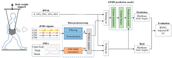
Figure 1.
Flowchart of joint angle prediction.
2.2. AWDF Prediction Model
The proposed AWDF model addresses critical challenges in predicting lower-limb joint angles during BWST, where neuromuscular activation patterns exhibit non-stationary characteristics under varying BWSLs. Traditional Fourier-based methods inadequately resolve the time–frequency tradeoff for dynamic sEMG signals, while fixed-threshold wavelet denoising often discards motion-relevant high-frequency components.
As shown in Figure 2, preprocessed sEMG signals are concurrently fed into two parallel modules: a LSTM network to capture temporal neuromuscular activation patterns, and an adaptive wavelet threshold learning module (ADTLM) that dynamically adjusts denoising parameters based on BWSL conditions. These learned features are then fused with real-time joint kinematics and BWSL vectors at the feature level, forming a hybrid representation that encodes both neuromuscular dynamics and biomechanical context. The fused features are processed through fully connected layers to predict lower-limb joint angles, explicitly compensating for electromechanical delay through phase-shifted labeling. In general, the end-to-end AWDF model eliminates the manual feature engineering of sEMG signals by employing a learning mechanism that autonomously extracts and filters discriminative sEMG features through wavelet coefficient optimization. By passing subjective human-designed feature thresholds, the model integrates sEMG/IMU inputs with kinematic outputs via a unified training framework, enabling automatic gradient propagation across wavelet denoising layers and kinematic decoders.
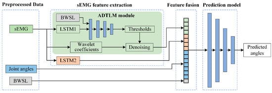
Figure 2.
Architecture of the proposed AWDF model for joint angle prediction.
2.2.1. ADTLM-Based Features
The proposed ADTLM addresses sEMG non-stationarity signals during BWST through a hybrid architecture combining LSTM-based temporal modeling and adaptive wavelet denoising. As depicted in Figure 2, the module processes preprocessed four-channel sEMG sliding window data alongside BWSL inputs.
Discrete wavelet transform (DWT) enables multiscale time-frequency analysis of nonstationary signals like sEMG. Unlike Fourier transform, DWT does not require signal stationarity assumptions and preserves localized temporal and spectral features through dyadic scaling and translation operations. Its hierarchical decomposition isolates neuromuscular activation patterns across frequency sub-bands while maintaining computational efficiency [21,28,29].
The DWT of a discrete signal
is defined as
where the basis function
is derived from its mother wavelet
by dilating and time-shifting. This relation can be defined as
where j, k, and n are integers, j is the depth of decomposition, and k is the translation parameter.
and
represent the scaling factor and the translation factor, respectively. Haar wavelets and Daubechies Db8 are commonly used mother wavelets, and this paper has employed both for experimental analysis.
For orthogonal or biorthogonal wavelets, the maximum decomposition level j is constrained by signal length L and filter length l [30]:
In this study, the obtained sEMG signals were decomposed by DWT level 3 decomposition according to Equation (3). For each sEMG channel, the signal yields one set of low-frequency coefficients and three sets of high-frequency coefficients derived from different decomposition scales, resulting in a total of 192 wavelet coefficient features.
The module architecture consists of a cascaded structure comprising an LSTM network and a fully connected network. The input to the model is preprocessed four-channel sEMG sliding window data along with BWSL inputs. The LSTM network extracts deep temporal features from the raw sEMG input to dynamically generate the denoising thresholds for wavelet coefficient selection, constructed by stacking two unidirectional LSTM layers, each containing 128 hidden units. The LSTM is intrinsically associated with wavelet feature selection because it automatically learns and dictates the thresholding parameters that determine which wavelet coefficients are retained (representing true neuromuscular activity) and which are discarded (considered noise). This adaptive process is superior to using fixed thresholds, especially under varying BWSLs where signal-to-noise characteristics change dynamically. The final hidden state of the LSTM is fed into the fully connected network to output wavelet thresholds. The fully connected network in ADTLM comprises three dense layers (256, 128, 64 nodes) with batch normalization (BN) and rectified linear unit (ReLU) activation. This hierarchical design progressively compresses temporal features extracted by LSTM into channel-specific thresholds, balancing nonlinear representation capacity and computational efficiency. The BN layers mitigate covariate shift during real-time operation, while ReLU ensures gradient stability in deep network training [19].
The ADTLM adaptively computes denoising thresholds by selectively weighting the wavelet coefficients of individual sEMG channels, where the number of output nodes equals the input channel count. This design preserves low-frequency wavelet coefficients representing neuromuscular activation trends while performing adaptive denoising on high-frequency components. Threshold determination involves two interdependent strategies: threshold selection and threshold function design.
We define the dynamic thresholds
for the decomposition level j of sEMG channel c, (c = 1–4) as
where
represents the adaptive denoising threshold output by for channel c and
denotes the wavelet high-frequency coefficients at decomposition level j for channel c.
This study employs soft thresholding denoising to preserve signal smoothness, where the denoised wavelet coefficients retain the capability to represent the original signal morphology [31]. Consequently, we adopt the soft thresholding method for denoising the high-frequency wavelet coefficients of sEMG signals; the threshold function mathematical definition is
where
denotes the sign function. Substituting this into Equation (4), we obtain the denoised wavelet coefficient features
after adaptive thresholding.
2.2.2. LSTM-Based Features
The LSTM is highly effective for processing time series data and has been proved to be suitable for regression problems in recent years [32]. Human lower-limb motion relies on sequential activation and inhibition of muscle groups to achieve coordinated joint angle transitions. sEMG signals reflect this neuromuscular coordination, where time-domain and frequency-domain features alone fail to capture cross-channel synergies. To address this limitation, we use LSTM architecture to learn the sEMG features. Figure 3a shows the memory channel and gate mechanism of the LSTM, including the cell state (which holds hidden state information for the current time step), the forgetting gate, input gate, update gate, and output gate. The hidden state integrates the previous time step’s hidden state and the current temporary state, while the gate structure regulates information flow by adding or removing content from the cell state. Let sEMG signal data
denote input at time t,
the prior hidden state, and
the previous cell state. The LSTM cell works as follows:
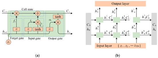
Figure 3.
LSTM-based feature learning. (a) LSTM cell, (b) dual-stacked LSTM network.
(1) Forget Gate Activation: Determines retention proportion of historical cell state, the forgotten gate reads
, and
and outputs a number between 0 and 1 for each cell state number.
(2) Input Gate Modulation: The input gate determines which new candidate state and be added to the cell state.
(3) Cell State Update: The function of the update gate is to transform old cell data
into new cell data
. Combines historical preservation and novel information.
(4) Output Gate Operation: After updating the cell state, the output cell state based on the input values
and
. The output
is the output vector result of the memory cell at the present and propagates to downstream layers and next timestep.
We propose a dual-stacked LSTM architecture, as shown in Figure 3b, where the input layer processes continuous sEMG signals through a sliding time window comprising 4 channels with 80 data points each, yielding an input dimension of 320.
In addition, Figure 2 shows the two specialized LSTM networks used in this work: LSTM1, with a 128-dimensional hidden layer output, focuses on wavelet coefficient threshold feature extraction, addressing signal variability induced by BWSL fluctuations. LSTM2 captures intra-channel temporal dependencies and inter-channel synergies across 4-channel sEMG inputs. The resulting 256-dimensional hidden state encodes muscle group activation patterns across the four sEMG channels, balancing computational efficiency with physiological coverage.
2.2.3. Feature Fusion and Prediction
The proposed AWDF module integrates four complementary modalities to address the challenges of attenuated sEMG activation patterns and BWSL-induced kinematic variability. As shown in ADTLM-based features, the derived denoised wavelet coefficients preserve high-frequency components for detecting transient neuromuscular activations while suppressing motion artifacts. LSTM-based features encode temporal dependencies and cross-channel interactions through stacked recurrent layers, effectively modeling muscle activation sequences [33]. Joint kinematics provide biomechanical priors to resolve ambiguity in weakened sEMG-force relationships under partial weight-bearing conditions [14]. BWSL dynamically recalibrates feature weights to adapt to gravitational unloading effects (i.e., reduced biomechanical load), ensuring consistent neuromuscular coupling across support levels. The fusion synergizes high-frequency sEMG resolution, temporal-spatial muscle coordination, kinematic constraints, and gravitational context, overcoming single-modality limitations such as motion artifact susceptibility and reduced sEMG discriminability under BWST. This framework achieves physiologically plausible feature representation while maintaining computational efficiency for real-time exoskeleton control.
The fused 1449-dimensional feature vector is processed through a fully connected network consisting of four sequential layers with 1024, 512, 128, and 64 hidden nodes, respectively. Each fully connected layer is followed by batch normalization to mitigate internal covariate shifts and accelerate training convergence, as well as a rectified linear unit (ReLU) activation function to introduce nonlinearity while avoiding gradient saturation. The progressive dimensionality reduction (1449→1024→512→128→64) balances feature abstraction and computational efficiency, enabling the network to hierarchically learn nonlinear mappings from multimodal inputs to joint angle kinematics. The final layer employs linear activation to output continuous predictions of hip and knee angles at future timesteps.
The proposed AWDF model employs an early fusion strategy, integrating denoised sEMG features, kinematic data, and BWSL parameters at the feature level before the final regression layers. An alternative paradigm is late fusion (or decision-level fusion), where predictions from multiple unimodal or simpler models are combined. To rigorously evaluate the superiority of our feature-level fusion approach, we implement late fusion models for comparative analysis [34,35].
2.3. Data Preprocessing
2.3.1. Filtering and Normalization
sEMG signals exhibit inherent susceptibility to multisource interference. Filtering is a standard procedure in sEMG signal processing, and to achieve optimal data processing outcomes, most research protocols prioritize the acquisition of raw signals followed by the tailored selection of filtering methods and parameters [21,22]. A zero-phase fourth-order Butterworth bandpass filter (20–450 Hz) was implemented to attenuate motion artifacts (<20 Hz) and high-frequency noise (>500 Hz) while preserving physiologically relevant spectral components. To mitigate 50 Hz powerline interference, a second-order IIR notch filter with ±2 Hz stopband was applied, achieving attenuation at the target frequency.
To address inter-channel amplitude variability and accelerate neural network convergence, Z-score standardization was applied per channel:
where
and
denote the channel-specific mean and standard deviation, respectively. This transformation ensures normalized input distributions (
,
) across all channels, a prerequisite for stable gradient computation in deep architectures. The normalization protocol effectively decouples amplitude variations caused by electrode-skin impedance differences from neuromuscular activation patterns [22].
2.3.2. Data Segmentation and Labeling
The selection of window length involves balancing signal information capture and latency. Overlapping analysis windows reduce data dimensionality and enhance computational efficiency. For physiological signal processing in motion prediction tasks, the literature suggests an optimal range of 100–250 ms, balancing temporal resolution and computational efficiency. We adopted a 160 ms window to optimize this tradeoff [11,12,13].
A sliding window protocol with 87.5% partial overlap was implemented for continuous angle prediction, the length of the sliding window was 160 ms, and the increment was 20 ms. The sEMG data were segmented into 160 ms windows (80 samples per channel at 500 Hz), while joint angles of hip and knee were interpolated to match the sEMG concatenating four-channel sEMG segments
and interpolated hip/knee joint angles
, yielding a 336-dimensional input vector:
where
denotes the instantaneous value from each sEMG channel and
denotes the calculated knee angles from IMU measurements.
As shown in Figure 4, conventional studies employed synchronous joint angle labeling (black point) relying on biomechanical signals as post hoc data labels [6,7,8,9,10]. To compensate for the electromechanical delay, we adopted a future-time labeling approach. The angle labels
(red point) were advanced by prediction time T. In this study, we evaluated T values ranging from 30 ms to 150 ms to determine the optimal prediction time, enabling an ahead-of-time control capability critical for exoskeleton applications.
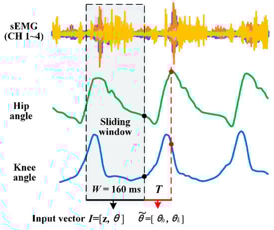
Figure 4.
Data window scheme and data labeling. Input vectors are labeled by angles measured by the IMU-calculated joint angle and the four-channel sEMG instantaneous value. W denotes window length. T denotes prediction time.
denotes the labeled angle.
2.4. Evaluation Criteria for the Models
To assess the performance of the proposed joint angle prediction model, three complementary metrics were adopted. Root mean square error (RMSE) quantifies the amplitude deviation between the predicted and actual joint angles, as seen in Equation (14). Pearson correlation coefficient (CC) evaluates the linear similarity of temporal patterns, with values closer to 1 indicating stronger phase synchronization, as seen in Equation (15). Adjusted R2 measures goodness-of-fit while penalizing model complexity to mitigate overfitting risks, as seen in Equation (16). This multi-metric approach addresses the limitations of single-criterion evaluations, balancing amplitude accuracy, temporal consistency, and model generalizability, while rigorous hypothesis testing identifies performance differences exceeding random variability. The calculation formulas are shown as follows:
where N is the number of samples and
represents the covariance between predicted angles
and real measured angles
.
and
correspond to the standard deviations of predicted and real measured angles, respectively. p indicates the number of input features in the prediction model.
2.5. Features Analysis for sEMG Signals
To comprehensively evaluate sEMG signals under different BWSL conditions, this study employs fractal dimension, sample entropy, and root mean square for multiscale characterization.
2.5.1. Fractal Analysis Via Higuchi’s Fractal Dimension
The application of fractal dimension in sEMG signal analysis provides a powerful framework for quantifying the inherent complexity and self-similarity of neuromuscular activities. Among various fractal dimension algorithms, Higuchi’s fractal dimension (HFD) stands out as a computationally efficient and physiologically interpretable metric for characterizing nonlinear dynamics in sEMG signals. This index, developed based on fractal theory, quantifies the complexity and irregularity of time series through multiscale curve length measurement. HFD exhibits high sensitivity to both local and global feature variations within time series, enabling it to capture complex signal information across different temporal scales. Higher HFD values reflect the greater signal irregularity that arises from asynchronous motor-unit firing patterns, which is indicative of nuanced neuromuscular control strategies [24,36,37]. HFD derivation involves the following:
(1) Reconstruction: For signal
, construct
new series:
where
stands for the initial time value,
denotes the discrete time interval between points.
(2) Length calculation: Compute the length of each new time series as defined above:
(3) Averaging: Compute the length of the curve for the time interval k as the average of the k values:
(4) Fractal dimension: Estimate HFD can be obtained by finding the slope of the curve of
versus
:
This study selects a 4 s window with a 500 Hz sEMG sampling frequency, resulting in sampling points
, and sets the maximum
.
2.5.2. Entropy Analysis Via Sample Entropy
Sample entropy (SampEn) quantifies the complexity and irregularity of physiological time series, reflecting neuromuscular adaptability under dynamic conditions, and captures amplitude-based irregularity in motor unit synchronization [23,25].
SampEn measures signal regularity by computing the conditional probability that similar amplitude sequences (m-length vectors) remain similar at the next point (m + 1), excluding self-matches to reduce bias. For an sEMG signal z(i), SampEn is calculated as follows:
(1) Define the template vectors:
(2) The distance between the
and
:
(3) The probability
that any
vector is close to
is determined. The
stands for a number of
vectors (1 ≤ j ≤ N − m, j ≠ i).
(4) The SampEn is negative logarithm of the conditional probability that two sequences similar for m points remain similar for the m + 1 points.
2.5.3. Time-Domain Analysis Via Root Mean Square
While SampEn and HFD capture nonlinear dynamics, the root mean square (RMS) provides time-domain energy normalization, RMS quantifies motor unit recruitment and myofiber discharge synchronization by computing the root mean square of sEMG signal amplitude [26].
Its calculation is defined as
where
denotes the sEMG signal in the k-th time window of the i-th channel and N represents the number of sampling points within the window. Its physiological relevance stems from directly reflecting motor unit recruitment and firing rate dynamics, where higher RMS values correlate with increased muscle force output during voluntary contractions.
3. Platform and Experiment
3.1. Human-Tracking Bodyweight Support System (BWSS)
Exoskeleton-integrated BWST has emerged as a neurorehabilitation breakthrough. Current clinical implementations predominantly utilize two architectural paradigms [2], as illustrated in Figure 5a: overhead rail-mounted systems with spatial constraints; and fixed treadmill-based configurations with limited gait variability.
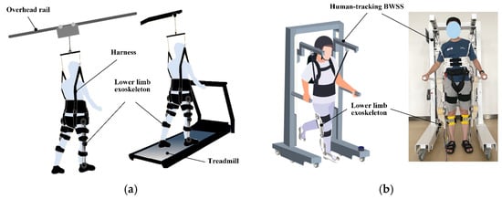
Figure 5.
Exoskeleton-integrated BWST. (a) Overhead rail-mounted and fixed treadmill-based BWSS. (b) Proposed overground exoskeleton-integrated BWSS.
Our research team has developed an overground exoskeleton-integrated BWSS, as shown in Figure 5b, which comprises two synergistic subsystems: human-tracking BWSS (mobile platform with real-time position synchronization) and lower-limb exoskeleton (powered joints for gait assistance). Exoskeleton has four active joints, hip/knee bilaterally, driven by brushless DC motors with harmonic drives to amplify torque output. All joints operate exclusively in the sagittal plane to provide physiological gait assistance during weight-supported training. The exoskeleton features length-adjustable thigh and shank segments to accommodate users across 155–185 cm height ranges. In contrast, the proposed robotic system enables a more natural overground walking pattern, thereby offering greater adaptability during rehabilitation training. The real-time BWSL adjustment through PID-controlled servo mechanisms, achieving across 0–40% BWSL via strain gauge feedback and lead screw actuation. The system’s mobile platform maintains human-tracking accuracy within 10 cm positional tolerance during dynamic locomotion while enabling natural walking pattern rehabilitation synchronization.
Figure 6 details the developed human-tracking BWSS. The robotic system detects slider displacement along linear guide rails using laser displacement sensors, enabling precise human motion perception. Synchronized motion tracking is achieved through servo motors, while tension sensors continuously monitor bodyweight support force. A screw motor dynamically regulates this force via closed-loop control. The system architecture comprises four integrated subsystems for power delivery, multimodal sensing, real-time control, and electromechanical actuation.
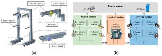
Figure 6.
Composition of the proposed human-tracking BWSS. (a) Structural composition. (b) Block diagram of the developed system.
3.2. Signal Acquisition System
In this study, sEMG signals and IMU data were synchronously acquired through the integrated system illustrated in Figure 7.

Figure 7.
Signal acquisition system. (a) The positions of IMUs and sEMG electrodes. (b) Subject wearing the acquisition system with human-tracking BWSS. (c) Composition of the signal acquisition system.
sEMG signals from the right lower-limb were captured using a four-channel wired acquisition system (Sichiray Co., Ltd., Kunshan, China) equipped with pre-gelled Ag/AgCl electrodes. The system operated at a sampling rate of 500 Hz, with a signal amplification gain of 2000 and a 12-bit analog-to-digital converter resolution. The electrodes were placed on the muscle bellies of four critical locomotor muscles after standard skin preparation, cleaning with alcohol swabs, to ensure inter-electrode impedance below 3 kΩ.
Joint kinematics were captured using three wireless IMU sensors (WT901WIFI, Wit Motion Co., Ltd., Shenzhen, China). Each IMU, streaming data at 100 Hz, integrates a triaxial accelerometer with a range of ±16 g, a triaxial gyroscope with a range of ±2000°/s, and a triaxial magnetometer. The sensors were calibrated prior to data collection using the manufacturer’s proprietary procedure to minimize offset and scale factor errors.
The raw data were streamed at 100 Hz via a WIFI connection to a host router and then forwarded to an embedded industrial computer. The orientation data output by the sensors were used to compute hip and knee joint angles. A multi-unit parallelization strategy was implemented using serial communication cables (23,400 bps baud rate) for the sEMG system, achieving stable 500 Hz real-time sampling via an Arduino UNO microcontroller-based signal conditioning hardware. Temporal synchronization across all sensor nodes (sEMG and IMU) was ensured through a hardware-triggered timestamp alignment protocol implemented on the industrial computer. A custom Python 3.12 script sent a simultaneous start command and generated a shared trigger pulse; temporal synchronization across all sensor nodes was ensured through hardware triggered timestamp alignment implemented on the industrial computer, maintaining inter-device clock deviation below 1 ms during trials.
The human upper body, thigh, and shank were simplified into a three-link mechanism, as shown in Figure 7a.
is the rotation matrix of the upper body relative to the thigh.
is the rotation matrix of the thigh relative to the shank.
are the rotation matrixes of three links relative to the ground, and can be calculated using an algorithm of the Euler-angle-to-rotation matrix based on IMU dates. Consequently, the hip and knee joint angles were derived using an algorithm for converting rotation matrices to Euler angles, as defined in Equations (27) and (28):
3.3. Experimental Protocol
Ten subjects (5 males and 5 females; age range: 23–27 years; mass range: 60–75 kg; height range: 158–182 cm), who had no history of lower-limb disorders, volunteered to participate in the experiment. All experiments were approved by the Ethical Committee of Anhui University of Science and Technology, and all participants provided written informed consent before the experiment.
As shown in Figure 7, the subject wore the multisource signal acquisition system and walked on the ground with a natural gait pattern while the developed bodyweight support system followed them automatically. The BWSLs were set to 0%, 10%, 20%, 30%, and 40% in this study. The maximum support level 40% was based on the clinic study about bodyweight supported training on gait rehabilitation [2]. Four muscles from one leg were selected to incorporate most functional muscles relative to normal walking, including rectus femoris (RF), vastus lateralis muscle (VL), biceps femoris (BF), semitendinosus (ST). Subjects were first required to become familiar with the experimental equipment, and walked along a straight for 8 m walkway on a flat ground environment. Each participant completed two consecutive trials under each BWSL, yielding 100 datasets (10 participants × 5 BWSLs × 2 trials). To mitigate muscle fatigue and ensure data reliability, a 5 min rest interval was enforced after each BWSL condition.
The sEMG signal precedes muscular contraction by about 50–100 ms and occurs approximately 30–150 ms prior to the actual movement [4]. The current sEMG features represent the movement of the future moment, and we use prediction time to compensate the electromechanical delay during model training. To assess the influence of prediction time and define its optimal range, six intervals were selected (30 ms, 60 ms, 90 ms, 120 ms, and 150 ms), aligning with physiological electromechanical delay ranges and data synchronization requirements.
To evaluate the predictive performance of the proposed model, a Leave-One-Out Cross-Validation (LOOCV) protocol was implemented. In each iteration, one participant’s dataset served as the test set, while data from the remaining four participants were used for training. The model was trained using the Adam optimizer with an initial learning rate of 0.0001, a batch size of 128, and 2000 epochs. Computational implementation utilized PyTorch 2.1.0 on a system equipped with an Intel i5-12700K CPU (Intel Corporation, Santa Clara, CA, USA), 64GB DDR5 RAM (Samsung Corporation, Suwon, Republic of Korea), and an NVIDIA GeForce RTX 4080 GPU (NVIDIA Corporation, Santa Clara, CA, USA). Training convergence was monitored using real-time visualization of loss landscapes and gradient distributions. Four ablation baseline models were systematically constructed to isolate feature contributions and evaluate the effectiveness of the proposed AWDF model. A one-way ANOVA was used to determine whether there was a statistically significant difference between the models in the ablation study.
(1) sEMG-based model: Integrated LSTM2-based sEMG features with BWSL parameters, serving as the foundational architecture for neuromuscular activation pattern analysis.
(2) Kinematic fusion model: Augmented the EMG-baseline model by incorporating real-time joint angle feedback through biomechanical sensor fusion.
(3) Wavelet-enhanced fusion model: Introduced threshold-free wavelet denoising coefficients to the kinematic fusion framework. This configuration validated the AWDF’s core innovation in adaptive bodyweight support influence while preserving transient neuromuscular activation characteristics.
(4) Late fusion model: This method first generated independent joint angle predictions from three separate models, each trained exclusively on one feature subset: ADTLM-based features, LSTM-based features, or joint kinematic features. The final prediction was then obtained by a learnable weighted fusion of these three model outputs.
In summary, the experimental protocol systematically analyzed three critical factors across five prediction time horizons (30–150 ms at 30 ms increments), five BWSLs (0–40% in 10% increments), and five prediction models (sEMG-based model, kinematic fusion model, wavelet-enhanced fusion model, late fusion model), and five prediction models (sEMG-based model, kinematic fusion model, wavelet-enhanced fusion model, late fusion model, and the proposed AWDF model)..
4. Results
4.1. Results of Gait Cycle and Muscle Activation with BWSLs
Analysis of gait cycle duration, normalized sEMG RMS variations, and factual analysis across incremental BWSLs revealed distinct neuromuscular adaptation patterns. As shown in Figure 8a,b, gait cycle duration progressively increased from 1.01 s at 0% BWSL to 1.57 s at 40% BWSL, indicating prolonged muscle activation intervals during BWST. Muscle-specific RMS analysis demonstrated heterogeneous neuromuscular responses: RF and VL muscles exhibited an initial decline from 0% to 20% BWSL, a subsequent increase at 30% BWSL, and a final reduction at 40% BWSL in RMS values, resulting in an overall downward trend. Conversely, ST muscle RMS values showed a progressive increase from 0% to 30% BWSL followed by gradual reduction at 40% BWSL. Notably, BF muscle activation followed a U-shaped trajectory, reaching minimal RMS at 20% BWSL before increasing at higher BWSLs. These findings quantitatively characterize the differential effects of BWSL modulation on temporal gait parameters and muscle activation intensity during BWST.
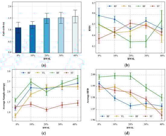
Figure 8.
Influence on gait cycle and muscle activation features with BWSLs. (a) Gait cycle variation, (b) sEMG RMS variation, (c) variation in of SampEn, (d) variation in average HFD.
As shown in Figure 8c, SampEn analysis was performed on the sEMG data from all channels and across all subjects under different BWSL conditions. The analysis was conducted with embedding dimension m = 2 and tolerance r = 0.5, as seen in Equations (22)–(25). The sample entropy metric, which quantifies the irregularity and predictability of sEMG time series data, was evaluated for four muscles. BF and RF exhibit a statistically significant increase in sample entropy within the 0–10% BWSL range, indicating heightened signal complexity during initial unloading phases; however, this trend stabilizes without notable changes in the subsequent 10–40% BWSL interval. In contrast, ST demonstrates no significant alterations in entropy across the entire BWSL spectrum, reflecting consistent neuromuscular control irrespective of support adjustments. For VL, sample entropy rises significantly from 0 to 20% BWSL, but plateaus beyond this point, showing minimal variation in higher support levels.
The average HFD was calculated for the sEMG signals across varying BWSLs for all subjects. The resulting HFD values for each muscle under different BWSL conditions are presented in Figure 8d. Overall, the HFD exhibited a general decreasing trend as the BWSL increased. Specifically, within the 0–10% BWSL range, the HFD values across muscles remained relatively stable with minimal changes. However, in the 10–40% BWSL range, a statistically significant decreasing trend in HFD was observed. The decrease in HFD values reflects alterations in the complexity and self-similarity properties of the neuromuscular signals. This reduction suggests a simplification of the motor control strategy or a loss of adaptive variability in muscle activation patterns under higher levels of bodyweight support.
4.2. Results of Model Prediction with Increased Prediction Time
To systematically evaluate the influence of prediction time window duration on joint angle prediction accuracy, we conducted comparative analyses of RMSE, CC, and Adjusted R2 across multiple time intervals (30–150 ms) using the AWDF model and ablation baseline models. Figure 9a–c demonstrates the performance degradation patterns across metrics as prediction time increases, with different colors denoting different prediction models.
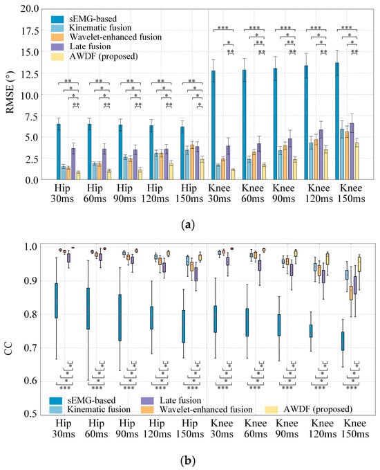
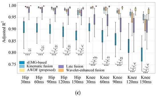
Figure 9.
Results of model prediction with increased prediction time. (a) RMSE, (b) CC, (c) Adjusted R2 (*, p < 0.05. **, p < 0.01. ***, p < 0.001).
As shown in Figure 9a, for hip joint predictions, the AWDF model achieved the best RMSE value 0.99° at 30 ms, compared to the sEMG-based model 6.31°, the kinematic fusion model 1.49°, and the Wavelet-enhanced fusion model 1.25°, respectively. A significant difference exists between the AWDF model and other ablation baseline models (p < 0.05). For knee joint predictions, the AWDF model maintains significant advantages over the sEMG-based model (p < 0.001) and the Wavelet-enhanced fusion model (p < 0.05). The AWDF model achieved the best RMSE value 1.23° at 30 ms, compared to sEMG-based model 12.72°, kinematic fusion model 2.08°, and Wavelet-enhanced fusion model 2.48°, respectively. However, the AWDF model shows marginal differences with the kinematic fusion model at 30 ms (p > 0.05). In general, the averaged RMSE of all prediction models presents a generally increasing trend as the prediction time increases.
Figure 9b reveals a progressive decline in CC value for all models as prediction time increased from 30 ms to 150 ms. The best results are 0.997 for 30 ms with hip angle prediction and 0.992 for 30 ms with knee angle prediction using the AWDF model, respectively. The AWDF model has a significant difference between other ablation baseline models (p < 0.05) for hip angle prediction. The statistical analysis shows that there is also no significant difference between the AWDF model and kinematic fusion model for 120 ms and 150 ms with knee prediction (p > 0.05).
Figure 9c reveals a progressive decline in averaged Adjusted R2 for all models as prediction time increased from 30 ms to 150 ms. The best results are 0.998 for 30 ms with hip angle prediction and 0.995 for 30 ms with knee angle prediction using the AWDF model, respectively. The AWDF model shows significant differences compared to most other ablation baseline models (p < 0.05) for both hip and knee angle predictions.
To systematically evaluate the temporal adaptability of the proposed AWDT model, we quantified its joint angle prediction performance across incremental prediction. As illustrated in Figure 10a,b, both hip and knee joint predictions exhibited time-dependent performance degradation. The hip joint demonstrated an RMSE escalation from 0.99° at 30 ms to 2.57° at 150 ms, while knee joint errors increased from 1.15° to 4.34° over the same interval. CC and Adjusted R2 exhibited analogous decay trends, with hip joint correlations declining from 0.996 to 0.964 and Adjusted R2 from 0.998 to 0.982, while knee joint metrics followed a comparable deterioration. A pronounced inflection point emerged at 90 ms, where RMSE, CC, and Adjusted R2 began to change significantly; therefore, this point was selected as the optimal prediction time in this study.
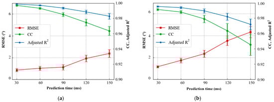
Figure 10.
The prediction performance of AWDF model with increased prediction time. (a) Hip angle prediction. (b) Knee angle prediction.
4.3. Results of Model Prediction with BWSLs
Building upon the optimized 90 ms prediction window established in prior analyses, we systematically evaluated the AWDF model against three ablation baselines under incremental BWSLs, 0–40%. Figure 11a–c illustrates the RMSE, CC, and Adjusted R2 distributions across hip and knee joints, revealing critical insights into BWSLs-dependent prediction dynamics.
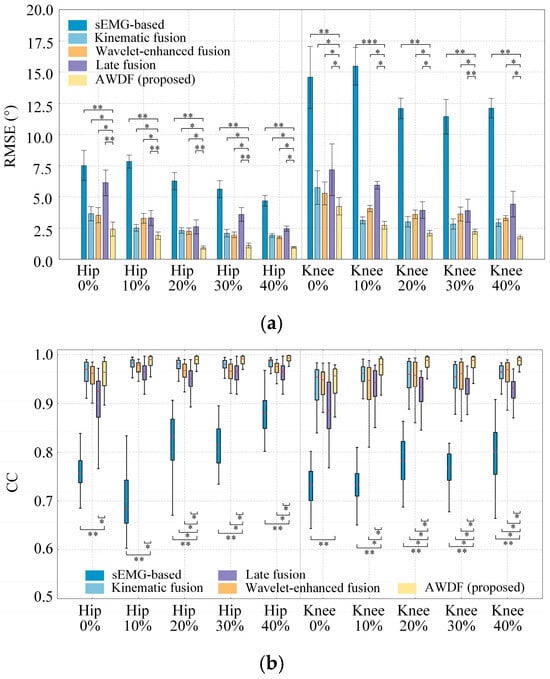
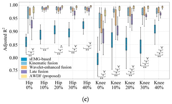
Figure 11.
Results of model prediction with BWSLs for different models. (a) RMSE, (b) CC, (c) Adjusted R2. Statistically significant difference (*, p < 0.05. **, p < 0.01, ***, p < 0.001).
As shown in Figure 11a, the RMSE of models presents a generally decreasing trend as the BWSL increases. The AWDF model demonstrates superior RMSE values across all BWSLs compared to sEMG-based (p < 0.01), kinematic fusion (p < 0.05), and Wavelet-enhanced models (p < 0.05) for hip angle prediction. Additionally, the statistical analysis shows that there is no significant difference (p > 0.05) between the AWDF model and the kinematic fusion model at knee prediction 10–30%. The best hip and knee prediction RMSE results are 1.14° and 2.06° at 40%, respectively.
As shown in Figure 11b, the AWDF model achieved CC values of hip and knee, significantly outperforming the sEMG-based (p < 0.01) across all BWSLs. For knee angle prediction, the AWDF model also showed a significant difference with the kinematic fusion and the Wavelet-enhanced models (p < 0.05). But for hip prediction, the difference between kinematic fusion and Wavelet-enhanced models appears at high BWSL, 20–40%. The best hip and knee prediction CC results by the AWDF model are 0.988 and 0.976 at 40%, respectively. In general, the CC values generally increase as BWSL increases.
In Figure 11c, the Adjusted R2 also generally increased as BWSL increases. The AWDF model achieves significant outperformance in Adjusted R2 values compared to the sEMG-based model for both hip and knee predictions (p < 0.01). Across the most BWSLs in hip and knee prediction, the AWDF model exhibits a significant advantage. The best hip and knee prediction of Adjusted R2 results using the AWDF model are 0.994 and 0.991 at 40%, respectively.
Figure 12a–e illustrates the hip and knee joint angle prediction trajectories for one subject across incremental BWSLs, 0–40%, with distinctive color-coded trajectories representing the performance of the AWDF model versus ablation prediction models. The 5 s test set excerpts demonstrate AWDF’s superior kinematic fidelity, showing near-perfect alignment with real joint angle measurements. In general, all prediction models exhibited progressive accuracy improvements with increasing BWSL. Analysis of continuous joint angle trajectories reveals a progressive prolongation of gait cycle duration with increasing BWSLs. Specifically, the mean gait cycle duration increased from 1.01 s at 0% BWSL to 1.57 s at 40% BWSL, with sEMG analysis revealing corresponding extensions in muscle activation durations across all channels.
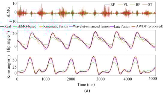
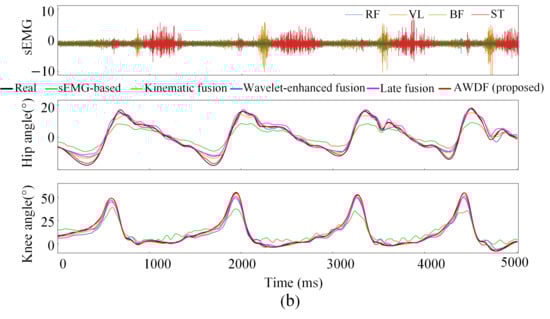
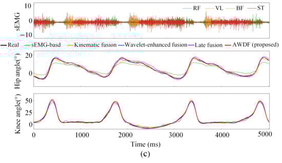
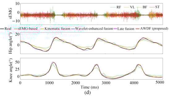
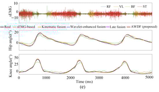
Figure 12.
Results of joint angle prediction with BWSLs of one subject: (a) 0% BWSL, (b) 10% BWSL, (c) 20% BWSL, (d) 30% BWSL, (e) 40% BWSL.
The predictive performance of the proposed AWDF model was quantitatively evaluated against comparative models through aggregated test set predictions across all BWSLs from five subjects. As shown in Table 1, the AWDF model demonstrates superior performance in both hip and knee joint angle predictions compared to baseline models. Specifically, achieving a lower RMSE of 1.073°–4.923° for hip and 0.907°–10.516° for knee, improving higher CC values of 0.008–0.190 for hip and 0.021–0.212 for knee, and enhancing Adjusted R2 values of 0.009–0.099 for hip and 0.018–0.137 for knee. These results indicate the AWDF model’s consistent advantage in minimizing prediction errors while maintaining robust correlation and goodness-of-fit with real joint angle measurements.

Table 1.
Average prediction metrics of BWSLs for different models.
4.4. Ablation and Sensitivity Analysis for AWDF
To justify the architectural choices of the proposed AWDF model, we conducted a series of ablation and sensitivity analyses. This section investigates the impact of two critical hyperparameters: the depth of the stacked LSTM network and the type of mother wavelet used in the ADTLM.
The performance of the AWDF model with varying LSTM depths (1–5 layers) was evaluated under the optimal 90 ms prediction horizon. The results are summarized in Table 2, and the two-layer LSTM configuration consistently achieved the best performance. Conversely, deeper networks (three or more layers) showed no further improvement, and even a slight degradation in performance, indicative of increased risk of overfitting and computational overhead without corresponding gains in predictive accuracy. Therefore, the two-layer architecture was selected as the optimal tradeoff.
Table 2.
Ablation and sensitivity analysis of model parameters.
Furthermore, the choice of the mother wavelet was critically examined by comparing the Daubechies Db8 against the Haar wavelet. The Db8 wavelet yielded statistically superior results, and this performance advantage is attributed to Db8’s smoother shape and better frequency localization, which are more suited to the non-stationary character of sEMG signals.
In conclusion, the sensitivity analyses confirm that the specific hyperparameters chosen for the final AWDF model—a two-layer LSTM and the Daubechies Db8 wavelet—are not arbitrary, but are empirically optimal for the task of joint angle prediction under BWST conditions. These design choices contribute directly to the model’s robust performance.
5. Discussion
5.1. Performance of Joint Angle Prediction with Various BWSLs
This study investigates joint angle prediction performance during BWST and demonstrates an enhancement in joint angle prediction accuracy with increasing BWSLs, a trend consistently observed across all evaluated models (Figure 11). While the existing literature extensively documents BWST applications, to our knowledge, this study represents the first systematic investigation of joint angle prediction under BWST experimental conditions.
As detailed in Section 4.1, BWST significantly alters gait patterns and sEMG characteristics, and increasing BWSL prolongs gait cycle duration and modifies RMS values of muscle activations. Previous studies have established BWSL-dependent biomechanical changes. Kristiansen et al. [15] demonstrated differential activation patterns in lower-limb muscles during BWSL escalation, with most muscles exhibited reduced activation intensities, while others like the BF displayed non-monotonic variations, which aligns with our results shown in Figure 8b. Similarly, Liu et al. [14] reported BWSL-dependent changes in lower-limb kinematics and muscular properties, notably, a BWSL-correlated reduction in step frequency, which aligns with our findings demonstrated in Figure 8a. While previous studies collectively confirm BWST’s biomechanical impacts, the key findings of our study reveal a counterintuitive relationship between BWSL modulation and prediction accuracy: despite progressive reductions in bodyweight, from 0% to 40%, joint angle prediction performance exhibited significant improvements.
From a rehabilitation perspective, this finding has significant implications. The enhanced prediction accuracy under higher BWSL conditions suggests that adaptive exoskeleton control may be most effective during early rehabilitation phases when bodyweight support is maximized. This aligns perfectly with clinical rehabilitation paradigms, where support is gradually reduced as patient capability improves. Our results provide a computational foundation for developing BWSL-aware control strategies that can dynamically adjust prediction models based on support levels.
The AWDF model’s ability to maintain high prediction accuracy across varying BWSL conditions demonstrates its robustness in handling these fundamental changes in neuromuscular dynamics. By adaptively filtering sEMG features and integrating multimodal data, the model effectively captures the essential neuromuscular information relevant for prediction, regardless of the support level. This adaptability underscores the importance of developing BWSL-aware algorithms for robust human–robot interaction in adaptive rehabilitation scenarios.
5.2. Analysis of Joint Angle Prediction in Advance
The extension of prediction time can mitigate electromechanical system delay; our study reveals a progressive degradation in prediction accuracy with longer time intervals. As shown in Table 3, Yi et al. [38] quantified this tradeoff, demonstrating performance degradation in LSTM models as prediction time increased, with optimal intervals identified at 54–81 ms. Fu et al. [20] investigated the impact of varying prediction horizons on joint angle prediction accuracy using Deep-STF model, suggesting an optimal prediction horizon of 250 ms for continuous ambulatory scenarios. Song et al. [18] systematically evaluated the impact of prediction horizons on LSTM-based joint angle prediction accuracy, reporting a progressive degradation in prediction fidelity with extended prediction intervals, achieving optimal performance at 50 ms.
Table 3.
Comparation with previous studies on prediction time.
The present study identified an optimal prediction time of approximately 90 ms, diverging from previous studies, notably, a difference of 250 ms. This discrepancy arises because discrete locomotion modes prediction using plantar pressure sensors necessitated extended prediction horizons, inherently requiring a longer prediction horizon compared to IMU-driven continuous kinematic tracking systems. Furthermore, the various prediction model may lead to different optimal prediction horizons. These results emphasize that prediction horizon selection represents a tradeoff between electromechanical delay compensation (requiring longer horizons) and motion intention prediction performance (favored by shorter horizons). The determination of optimal prediction time is influenced by sensor system heterogeneity, task-specific requirements, and model architectural variations. However, we choose the pronounced inflection points that emerged at 90 ms, where RMSE, CC, and Adjusted R2 start to change significantly. The inflection point is not the only standard to decide optimal prediction time; it depends on the delay of the deployed exoskeleton system. In this study, the inference time of executing the proposed AWDF algorithm is about 12 ms, achieved using a CPU i5-12700K and GPU GeForce RTX 4080. Therefore, the prediction time is large enough to cover the execution of the prediction algorithm and still leaves enough room for compensating the mechanical transmission delay.
5.3. Effectiveness of the Proposed AWDF Prediction Model
This study proposes an AWDF model to address joint angle prediction under varying BWSLs. The AWDF model integrates adaptive threshold denoising for sEMG wavelet coefficients, along with multimodal fusion of sEMG, joint angle kinematics, and BWSL features. Comparative experiments with four baseline models demonstrate AWDF’s superior accuracy and effectiveness. As shown in Figure 9 and Figure 11, results indicate that the sEMG-based model (solely relying on LSTM features) exhibited the lowest prediction accuracy, highlighting the limitations of isolated sEMG features for BWST applications. Incorporating joint angle kinematic features significantly improved prediction performance, validating the positive effects of feature fusion. To further verify the efficacy of the ADTLM in sEMG feature learning, the wavelet-enhanced fusion model was compared against the AWDF. Experimental results confirm the superiority of the ADTLM in automatically selecting threshold-filtered wavelet coefficients with higher relevance to prediction tasks.
As shown in Table 1, the superior performance of the proposed AWDF model over the late fusion variants underscores a key advantage of feature-level fusion for this specific continuous regression task. While late fusion strategies like graph-regularized combination are powerful for classification, their comparative shortcomings here can be attributed to a fundamental limitation: the loss of rich, cross-modal information during the intermediate decision-making stage [34,35]. In contrast, our AWDF model’s early fusion strategy integrates these heterogeneous data streams before they are transformed into predictions. This allows for the model to learn a unified, discriminative feature representation where interactions between a specific sEMG pattern, a particular joint angle, and a given BWSL can be directly discovered and exploited by the subsequent nonlinear mapping network. Comprehensive comparisons demonstrate that the AWDF model adaptively accommodates BWSL variations during BWST application, thereby improving joint angle prediction accuracy.
Although joint angle estimation and joint angle prediction represent distinct conceptual frameworks, their divergence primarily manifests in data labeling protocols rather than fundamentally impacting regression models’ inherent performance. To broaden comparative analyses, this study disregards these distinctions; relevant studies are illustrated in Table 4. Adjusted R2 and R2 values are consolidated into a single column, with RMSE metrics rounded to two decimal places. Existing studies employ diverse regression models for joint angle prediction (estimation); however, the proposed AWDF model does not achieve optimal performance across all benchmarks. BWST conditions and prediction time horizons are identified as critical factors influencing model efficacy. Nevertheless, the AWDF model prediction satisfies the fundamental accuracy requirements for lower-limb exoskeleton control applications.
Table 4.
Comparation with previous studies on joint angle prediction (estimation).
The ablation studies further substantiate the AWDF model’s design. As shown in Table 2, the superiority of the Db8 wavelet over Haar confirms that a wavelet matched to sEMG’s non-stationary nature—with better frequency localization—yields more physiologically relevant features. Conversely, the Haar wavelet’s discontinuous nature proved to be less capable of preserving these subtle patterns. Similarly, the optimal performance of the two-layer LSTM suggests that this depth sufficiently captures the temporal dynamics of muscle synergies without over-parameterization. Thus, the model’s efficacy is rooted in these principled, validated architectural choices.
5.4. Fractal Nature of Muscle Control Under BWST: Insights from HFD Analysis
While RMS and SampEn remain valuable indicators of muscle activation intensity and signal irregularity, respectively, their responses to BWSL variations in our study were heterogeneous and less consistent. In contrast, HFD demonstrated a strong, systematic negative correlation with increasing BWSL across all conditions, underscoring its superior utility as an indicator of neuromuscular adaptation under dynamic unloading. The unique capability of HFD makes it a promising indicator for decoding neuromuscular adaptations under dynamic unloading.
The theoretical supremacy of HFD stems from its ability to quantify the fractal nature—the self-similarity and complexity—of the underlying motor control strategy. The observed decrease in HFD signifies a fundamental simplification and regularization of the neural drive to muscles as BWSL increases. This suggests that, under reduced biomechanical load, the central nervous system adopts a more stereotyped and less adaptive motor unit recruitment pattern [26,43]. Thus, the reduction in HFD provides a profound explanation for the BWSL-induced changes: it reveals a shift in the fractal characteristics of the control signal itself, marking a transition towards a simpler neuromuscular control regime.
Furthermore, the exceptional performance of our AWDF model can be reinterpreted through this lens of fractal analysis. The model’s core innovation lies in its adaptive wavelet thresholding, which is inherently designed to preserve and leverage the fractal properties of the sEMG signal. By dynamically tuning its denoising parameters based on BWSL, the AWDF model effectively compensates for the loss of signal complexity (HFD decrease) quantified in our analysis. This intrinsic alignment between the model’s architecture and the fractal nature of the signal provides a deeper theoretical foundation for its superior prediction accuracy and cross-condition robustness.
5.5. Limitations and Future Directions
This study introduced a novel AWDF model for joint angle prediction during BWST, yet several limitations must be noted, pointing to clear avenues for future work.
First, while the inclusion of ten healthy young adults enhanced generalizability, the absence of clinical populations and older age groups remains a constraint. Future work will therefore prioritize clinical validation in patient cohorts to evaluate the model’s utility in real-world rehabilitation settings.
Second, the scope of this work was limited to overground walking in the sagittal plane. To assess the model’s full versatility, future studies will extend the framework to more complex tasks such as stair climbing, sit-to-stand transitions, and balance control. Additionally, the long-term repeatability of predictions and robustness to muscle fatigue during prolonged use warrants further investigation.
Third, although ablation studies justified key model choices and desktop tests confirmed computational feasibility, the model has not been deployed on embedded hardware. The critical next step is to port and validate the AWDF model on a portable exoskeleton system, ensuring real-time performance in a closed-loop control environment.
By addressing these aspects, the AWDF model can evolve from a proof-of-concept into a robust, clinically viable technology for adaptive neurorehabilitation.
6. Conclusions
This study presents a systematic investigation of continuous lower-limb joint angle prediction under dynamic BWST conditions. To address the unique challenges posed by varying BWSLs, an AWDF model was developed, integrating multimodal features from sEMG, IMU kinematics, and BWSL parameters. The core findings and contributions of this work are fourfold:
First, this study was the first to report and quantify a previously unreported phenomenon: joint angle prediction accuracy improves with increasing BWSL. This counterintuitive finding was analyzed through multidimensional perspectives, revealing that reduced gravitational load leads to a simplification of neuromuscular control, which in turn yields more predictable sEMG patterns for data-driven models.
Second, the proposed AWDF model demonstrated superior performance and robust cross-condition adaptability against several baseline models. The average RMSE, CC, and Adjusted R2 for hip and knee angle prediction are 1.468°–2.626°, 0.983–0.973, and 0.992–0.986, respectively. Its novel adaptive wavelet thresholding module effectively preserves discriminative neuromuscular features while mitigating noise induced by BWSL variations, establishing a new state-of-the-art framework for BWST applications.
Third, the influence of prediction time was thoroughly explored, identifying an optimal prediction horizon of 90 ms that effectively balances the compensation for system latency against the degradation in prediction accuracy. This finding provides a crucial design parameter for real-time exoskeleton control systems.
Fourth, using a multiscale feature analysis, we provide a novel interpretation of the fractal nature of neuromuscular control under BWST. The systematic decrease in HFD emerged as the most consistent biomarker, offering profound insights into how the central nervous system simplifies control strategies under reduced gravitational loading.
Author Contributions
Conceptualization, methodology, software, and writing, L.J.; validation, formal analysis, and investigation, Z.Y.; data curation, Y.L.; visualization, L.W.; supervision, project administration, and funding acquisition, L.L. writing—original draft preparation, L.J.; writing—review and editing, L.J.. All authors have read and agreed to the published version of the manuscript.
Funding
This work was supported in part by the Research and the Development Fund of the Institute of Environmental Friendly Materials and Occupational Health, Anhui University of Science and Technology, Grant/Award Number: ALW2022YF06.
Data Availability Statement
The raw data supporting the conclusions of this article will be made available by the authors on request.
Conflicts of Interest
The authors declare no conflicts of interest.
References
- Yang, F.-A.; Chen, S.-C.; Chiu, J.-F.; Shih, Y.-C.; Liou, T.-H.; Escorpizo, R.; Chen, H.-C. Body Weight-Supported Gait Training for Patients with Spinal Cord Injury: A Network Meta-Analysis of Randomised Controlled Trials. Sci. Rep. 2022, 12, 19262. [Google Scholar] [CrossRef]
- Yamamoto, R.; Sasaki, S.; Kuwahara, W.; Kawakami, M.; Kaneko, F. Effect of Exoskeleton-Assisted Body Weight-Supported Treadmill Training on Gait Function for Patients with Chronic Stroke: A Scoping Review. J. NeuroEng. Rehabil. 2022, 19, 143. [Google Scholar] [CrossRef]
- Siviy, C.; Baker, L.M.; Quinlivan, B.T.; Porciuncula, F.; Swaminathan, K.; Awad, L.N.; Walsh, C.J. Opportunities and Challenges in the Development of Exoskeletons for Locomotor Assistance. Nat. Biomed. Eng. 2022, 7, 456–472. [Google Scholar] [CrossRef]
- Li, L.-L.; Cao, G.-Z.; Liang, H.-J.; Zhang, Y.-P.; Cui, F. Human Lower Limb Motion Intention Recognition for Exoskeletons: A Review. IEEE Sens. J. 2023, 23, 30007–30036. [Google Scholar] [CrossRef]
- Yan, T.; Cempini, M.; Oddo, C.M.; Vitiello, N. Review of Assistive Strategies in Powered Lower-Limb Orthoses and Exoskeletons. Robot. Auton. Syst. 2015, 64, 120–136. [Google Scholar] [CrossRef]
- Lu, Y.; Wang, H.; Zhou, B.; Wei, C.; Xu, S. Continuous and Simultaneous Estimation of Lower Limb Multi-Joint Angles from sEMG Signals Based on Stacked Convolutional and LSTM Models. Expert Syst. Appl. 2022, 203, 117340. [Google Scholar] [CrossRef]
- Xi, X.; Jiang, W.; Hua, X.; Wang, H.; Yang, C.; Zhao, Y.-B.; Miran, S.M.; Luo, Z. Simultaneous and Continuous Estimation of Joint Angles Based on Surface Electromyography State-Space Model. IEEE Sens. J. 2021, 21, 8089–8099. [Google Scholar] [CrossRef]
- Qin, P.; Shi, X.; Zhang, C.; Han, K. Continuous Estimation of the Lower-Limb Multi-Joint Angles Based on Muscle Synergy Theory and State-Space Model. IEEE Sens. J. 2023, 23, 8491–8503. [Google Scholar] [CrossRef]
- Ling, L.; Wei, L.; Feng, B.; Lin, Z.; Jin, L.; Wang, Y.; Li, W. A Lightweight Multi-Scale Convolutional Attention Network for Lower Limb Motion Recognition with Transfer Learning. Biomed. Signal Process. Control 2025, 99, 106803. [Google Scholar] [CrossRef]
- Ling, L.; Wang, Y.; Ding, F.; Jin, L.; Feng, B.; Li, W.; Wang, C.; Li, X. An Efficient Method for Identifying Lower Limb Behavior Intentions Based on Surface Electromyography. Comput. Mater. Contin. 2023, 77, 2771–2790. [Google Scholar] [CrossRef]
- Foroutannia, A.; Akbarzadeh-T, M.-R.; Akbarzadeh, A. A Deep Learning Strategy for EMG-Based Joint Position Prediction in Hip Exoskeleton Assistive Robots. Biomed. Signal Process. Control 2022, 75, 103557. [Google Scholar] [CrossRef]
- Lu, Z.; Chen, S.; Yang, J.; Liu, C.; Zhao, H. Prediction of Lower Limb Joint Angles from Surface Electromyography Using XGBoost. Expert Syst. Appl. 2025, 264, 125930. [Google Scholar] [CrossRef]
- Han, J.; Tian, Y.; Wang, H.; Peyrodie, L. Continuous Limb Joint Angle Prediction from sEMG Using SA-FAWT and Conv-BiLSTM. Biomed. Signal Process. Control 2024, 97, 106681. [Google Scholar] [CrossRef]
- Liu, B.; Li, S.; Liang, B.; Xie, L. Exploring the Effects of Body Weight Support Systems on Lower Limb Kinematics and Muscle Characteristics. Biomed. Signal Process. Control 2023, 85, 104947. [Google Scholar] [CrossRef]
- Kristiansen, M.; Odderskær, N.; Kristensen, D.H. Effect of Body Weight Support on Muscle Activation during Walking on a Lower Body Positive Pressure Treadmill. J. Electromyogr. Kinesiol. 2019, 48, 9–16. [Google Scholar] [CrossRef]
- Bu, A.; MacLean, M.K.; Ferris, D.P. EMG-Informed Neuromuscular Model Assesses the Effects of Varied Bodyweight Support on Muscles during Overground Walking. J. Biomech. 2023, 151, 111532. [Google Scholar] [CrossRef]
- Kumar Das, S.; Das, N.; Chakraborty, M. Power Spectral Density, Higuchi’s Fractal Dimension and Detrended Fluctuation Analysis of sEMG at Varying Weights. In Proceedings of the 2023 International Conference on Computer, Electrical & Communication Engineering (ICCECE), Kolkata, India, 20 January 2023; pp. 1–7. [Google Scholar]
- Song, Q.; Ma, X.; Liu, Y. Continuous Online Prediction of Lower Limb Joints Angles Based on sEMG Signals by Deep Learning Approach. Comput. Biol. Med. 2023, 163, 107124. [Google Scholar] [CrossRef] [PubMed]
- Zhu, M.; Guan, X.; Li, Z.; He, L.; Wang, Z.; Cai, K. sEMG-Based Lower Limb Motion Prediction Using CNN-LSTM with Improved PCA Optimization Algorithm. J. Bionic Eng. 2023, 20, 612–627. [Google Scholar] [CrossRef]
- Fu, P.; Zhong, W.; Zhang, Y.; Xiong, W.; Lin, Y.; Tai, Y.; Meng, L.; Zhang, M. Predicting Continuous Locomotion Modes via Multidimensional Feature Learning from sEMG. IEEE J. Biomed. Health Inform. 2024, 28, 6629–6640. [Google Scholar] [CrossRef]
- Duan, F.; Dai, L.; Chang, W.; Chen, Z.; Zhu, C.; Li, W. sEMG-Based Identification of Hand Motion Commands Using Wavelet Neural Network Combined with Discrete Wavelet Transform. IEEE Trans. Ind. Electron. 2016, 63, 1923–1934. [Google Scholar] [CrossRef]
- Zafar, M.H.; Falkenberg Langås, E.; Sanfilippo, F. Human-Robot Interaction Using sEMG Sensor: Hybrid Deep Learning Model for Accurate Hand Gesture Recognition. Results Eng. 2023, 20, 101639. [Google Scholar] [CrossRef]
- Kosmidou, V.E.; Hadjileontiadis, L.J. Sign Language Recognition Using Intrinsic-Mode Sample Entropy on sEMG and Accelerometer Data. IEEE Trans. Biomed. Eng. 2009, 56, 2879–2890. [Google Scholar] [CrossRef] [PubMed]
- Armonaite, K.; Conti, L.; Laura, L.; Primavera, M.; Tecchio, F. Linear and Non-Linear Methods to Discriminate Cortical Parcels Based on Neurodynamics: Insights from sEEG Recordings. Fractal Fract. 2025, 9, 278. [Google Scholar] [CrossRef]
- Čukić, M.B.; Platiša, M.M.; Kalauzi, A.; Oommen, J.; Ljubisavljević, M.R. The Comparison of Higuchi’s Fractal Dimension and Sample Entropy Analysis of sEMG: Effects of Muscle Contraction Intensity and TMS. arXiv 2018. [Google Scholar] [CrossRef]
- Cui, W.; Chen, X.; Cao, S.; Zhang, X. Muscle Fatigue Analysis of the Deltoid during Three Head-Related Static Isometric Contraction Tasks. Entropy 2017, 19, 221. [Google Scholar] [CrossRef]
- Li, J.; Wang, C.; Su, W.; Ye, D.; Wang, Z. Uncertainty-Aware Self-Attention Model for Time Series Prediction with Missing Values. Fractal Fract. 2025, 9, 181. [Google Scholar] [CrossRef]
- Ait Yous, M.; Agounad, S.; Elbaz, S. Automated Detection and Removal of Artifacts from sEMG Signals Based on Fuzzy Infer-ence System and Signal Decomposition Methods. Biomed. Signal Process. Control 2024, 94, 106307. [Google Scholar] [CrossRef]
- Subasi, A. Classification of EMG Signals Using Combined Features and Soft Computing Techniques. Appl. Soft Comput. 2012, 12, 2188–2198. [Google Scholar] [CrossRef]
- Xiong, F.; Qi, X.; Nattel, S.; Comtois, P. Wavelet Analysis of Cardiac Optical Mapping Data. Comput. Biol. Med. 2015, 65, 243–255. [Google Scholar] [CrossRef]
- Guo, D.-F.; Zhu, W.-H.; Gao, Z.-M.; Zhang, J.-Q. A Study of Wavelet Thresholding Denoising. In Proceedings of the WCC 2000—ICSP 2000, 2000 5th International Conference on Signal Processing Proceedings, 16th World Computer Congress 2000, Beijing, China, 21–25 August 2000; IEEE: Beijing, China, 2000; Volume 1, pp. 329–332. [Google Scholar]
- Özçelik, Y.B.; Altan, A. Overcoming Nonlinear Dynamics in Diabetic Retinopathy Classification: A Robust AI-Based Model with Chaotic Swarm Intelligence Optimization and Recurrent Long Short-Term Memory. Fractal Fract. 2023, 7, 598. [Google Scholar] [CrossRef]
- Wang, Z.; Xiong, C.; Zhang, Q. Enhancing the Online Estimation of Finger Kinematics from sEMG Using LSTM with Attention Mechanisms. Biomed. Signal Process. Control 2024, 92, 105971. [Google Scholar] [CrossRef]
- Salazar, A.; Safont, G.; Vergara, L.; Vidal, E. Graph Regularization Methods in Soft Detector Fusion. IEEE Access 2023, 11, 144747–144759. [Google Scholar] [CrossRef]
- Gadzicki, K.; Khamsehashari, R.; Zetzsche, C. Early vs Late Fusion in Multimodal Convolutional Neural Networks. In Proceedings of the 2020 IEEE 23rd International Conference on Information Fusion (FUSION), Rustenburg, South Africa, 6–9 July 2020; IEEE: Rustenburg, South Africa, 2020; pp. 1–6. [Google Scholar]
- Li, Y.; Zhang, S.; Liang, L.; Ding, Q. Multivariate Multiscale Higuchi Fractal Dimension and Its Application to Mechanical Signals. Fractal Fract. 2024, 8, 56. [Google Scholar] [CrossRef]
- Ancillao, A.; Galli, M.; Rigoldi, C.; Albertini, G. Linear Correlation between Fractal Dimension of Surface EMG Signal from Rectus Femoris and Height of Vertical Jump. Chaos Solitons Fractals 2014, 66, 120–126. [Google Scholar] [CrossRef]
- Yi, C.; Jiang, F.; Zhang, S.; Guo, H.; Yang, C.; Ding, Z.; Wei, B.; Lan, X.; Zhou, H. Continuous Prediction of Lower-Limb Kinematics From Multi-Modal Biomedical Signals. IEEE Trans. Circuits Syst. Video Technol. 2022, 32, 2592–2602. [Google Scholar] [CrossRef]
- Sun, N.; Cao, M.; Chen, Y.; Chen, Y.; Wang, J.; Wang, Q.; Chen, X.; Liu, T. Continuous Estimation of Human Knee Joint Angles by Fusing Kinematic and Myoelectric Signals. IEEE Trans. Neural Syst. Rehabil. Eng. 2022, 30, 2446–2455. [Google Scholar] [CrossRef]
- Li, G.; Li, Z.; Su, C.-Y.; Xu, T. Active Human-Following Control of an Exoskeleton Robot With Body Weight Support. IEEE Trans. Cybern. 2023, 53, 7367–7379. [Google Scholar] [CrossRef]
- Shi, X.; Li, S.; Li, X.; Lu, H.; Tang, J. Research on Prediction of Human Lower Limb Joint Angle Based on sEMG Signal. IET Conf. Proc. 2025, 2024, 944–951. [Google Scholar] [CrossRef]
- Yang, J.; Lu, Z.; Chen, S.; Liu, C.; Zhao, H. Continuous Knee Joint Angle Prediction with Surface EMG. Biomed. Signal Process. Control 2024, 95, 106354. [Google Scholar] [CrossRef]
- Sriram, S.; Rajagopal, K.; Krejcar, O.; Namazi, H. DECODING OF THE EXTRAOCULAR MUSCLES ACTIVATIONS BY COMPLEXITY-BASED ANALYSIS OF ELECTROMYOGRAM (EMG) SIGNALS. Fractals 2024, 32, 2450067. [Google Scholar] [CrossRef]
Disclaimer/Publisher’s Note: The statements, opinions and data contained in all publications are solely those of the individual author(s) and contributor(s) and not of MDPI and/or the editor(s). MDPI and/or the editor(s) disclaim responsibility for any injury to people or property resulting from any ideas, methods, instructions or products referred to in the content. |
© 2025 by the authors. Licensee MDPI, Basel, Switzerland. This article is an open access article distributed under the terms and conditions of the Creative Commons Attribution (CC BY) license (https://creativecommons.org/licenses/by/4.0/).