Fractal–Fractional Coupled Systems with Constant and State- Dependent Delays: Existence Theory and Ecological Applications

Abstract

This study introduces a new class of coupled differential systems described by fractal–fractional Caputo derivatives with both constant and state-dependent delays. In contrast to traditional delay differential equations, the proposed framework integrates memory effects and geometric complexity while capturing adaptive feedback delays that vary with the system’s state. Such a formulation provides a closer representation of biological and physical processes in which delays are not fixed but evolve dynamically. Sufficient conditions for the existence and uniqueness of solutions are established using fixed-point theory, while the stability of the solution is investigated via the Hyers–Ulam (HU) stability approach. To demonstrate applicability, the approach is applied to two illustrative examples, including a predator–prey interaction model. The findings advance the theory of fractional-order systems with mixed delays and offer a rigorous foundation for developing realistic, application-driven dynamical models.

1. Introduction

Recent studies have increasingly focused on the inclusion of time delays in biological models to more accurately capture natural processes such as feeding intervals, maturation periods, resource renewal, and response delays. The presence of such lags introduces memory effects into the dynamics, which can significantly alter system behavior. Both classical and modern research (see [1,2,3,4]) have shown that delay differential equations (DDEs) are capable of producing complex phenomena, including instability, bifurcation, and persistent oscillations, primarily due to the influence of past states on current dynamics. Alongside application-driven investigations, notable theoretical progress has been made in the mathematical study of delay systems. For example, stability and bifurcation analysis of delay equations have been addressed in [5,6], and the discrete and proportional delay dynamics were analyzed by Shah et al. [7], who examined the qualitative behavior of a nonlinear delay problem and demonstrated the applicability of their approach to a realistic housefly population model. Furthermore, specialized numerical techniques for approximating solutions of delay equations are under active development [8]. Collectively, these works underscore that the interplay between differential operators and delay structures is not only essential for realistic modeling but also central to advancing rigorous theoretical foundations.

Many biologically inspired models inherently involve multiple discrete delays. Noteworthy cases include the well-known housefly population dynamics studied in [9] and the logistic model integrating Allee effects and dual time delays [10]. In addition, we examine complex systems in epidemiology [11], neuroscience [12], and medicine [13]. Such models are known for exhibiting a wide range of dynamic responses, often characterized by rich and intricate structures [14].

Traditional integer-order DEs typically fall short in accounting for memory-dependent or hereditary traits inherent in real-world systems. To bridge this gap, fractional-order differential models were introduced, employing nonlocal operators defined through integral kernels. The growing interaction between fractional calculus and practical modeling has significantly advanced the field, establishing fractional differential equations (FDEs) as an essential tool in modern applied mathematics. These equations are now widely employed in multiple domains, including physics, engineering, and technology. Their applicability extends to areas such as control systems, electrochemical dynamics, electromagnetic modeling, viscoelastic behavior, and transport through porous structures (see [15,16,17]). However, classical fractional formulations may prove insufficient in scenarios involving irregular geometries, fractal media, or anomalous transport phenomena. This growing interest has led to the adoption of fractal–fractional derivatives—particularly those in the Caputo sense, owing to memory kernels characterized by a power–law behavior. Unlike the classical Caputo derivative, which captures long-term memory effects through a power–law kernel, the actional Caputo derivative incorporates an additional fractal dimension parameter to model processes that simultaneously exhibit memory and fractality [18]. This operator becomes necessary when the underlying dynamics cannot be fully described by temporal memory alone, such as in ecological systems with irregular environmental heterogeneity or multi-scale interactions. For problems where the geometry of interactions or resource distributions is non-Euclidean, the fractal–fractional Caputo operator provides a more realistic description compared to its classical counterpart. In [19], the authors utilized fractal–fractional calculus to apply analytical methods for examining the dynamics of a breast cancer model, uncovering significant insights into disease progression. A similar approach was adopted in [20], where a waterborne disease model was analyzed using fractal–fractional operators. The work focused on both theoretical development and numerical simulations to better understand the system’s behavior. In [21], a model involving liver fibrosis was constructed within the framework of fractal–fractional derivatives, emphasizing transitions across subintervals and providing mathematical interpretations. Likewise, the study in [22] investigated the spread of Ebola using a Φ-piecewise hybrid fractional derivative framework. These developments reflect the growing reliance on advanced mathematical modeling to interpret and predict complex biological phenomena.

While most existing studies employ either constant fractional operators or classical integer-order delays, the present work advances this line of research by combining fractal–fractional derivatives with both constant and state-dependent delays. By explicitly incorporating these features, our system is capable of capturing a richer set of dynamical behaviors. Moreover, the inclusion of both constant and state-dependent delays is essential in faithfully modeling systems where the temporal lag is influenced by the evolving state, such as population density, stress, or infection load. In domains like biology, control systems, and medicine, state-dependent delays are particularly impacted. Integrating these delay structures with fractal–fractional calculus provides a comprehensive and flexible modeling framework that captures complex feedback interactions and memory-driven evolution in dynamical systems. This hybrid formulation addresses limitations in earlier models that often ignore scale-dependent effects or adaptive delay mechanisms.

On the other hand, systems of coupled DEs play a vital role in modeling complex systems where multiple variables interact dynamically over time. These systems arise naturally in diverse fields such as biology, physics, engineering, and economics. In particular, coupling allows for the representation of interdependent processes, such as predator–prey relationships in ecology. In particular, Tahara et al. [23] investigated the asymptotic stability of a modified Lotka-Volterra predator–prey system with small immigration effects, illustrating how subtle external inputs can influence long-term ecological equilibria perspective that parallels our stability analysis under adaptive delays. The mathematical framework of coupled equations captures the mutual influence between components, enabling a more realistic and comprehensive understanding of the system’s behavior. This approach provides valuable insights into synchronization, stability, bifurcations, and emergent phenomena that cannot be observed in single-equation models. As a result, the study of coupled differential systems is essential for accurately simulating and analyzing real-world interactions that involve feedback, cooperation, or competition between subsystems. In many research papers, coupled systems of DEs have been considered; for instance, see [24,25,26]. Recently, authors investigated existence and stability results of a coupled fractal–fractional DEs [27].

Recent progress in fixed point theory has provided powerful tools for establishing the existence and uniqueness of solutions in nonlocal and delay systems. For instance, Younis and Öztürk [28] presented novel proximal point results and their applications to nonlinear problems. Abdou [29] demonstrated how fixed-point techniques in orthogonal metric spaces can ensure solutions for nonlinear FDEs. Related foundational work by Alqahtani et al. [30] on extended b-metric spaces illustrates the broad applicability of generalized contraction frameworks. Although our study employs Banach and Schaefer theorems in a Banach space of continuous functions, these proximal and extended-metric approaches provide complementary tools that could be explored in future extensions.

In the literature, several numerical methods have been proposed for the solution of FDEs. Classical numerical schemes such as the Runge–Kutta family, predictor–corrector methods, and Adams–Bashforth variants have long been applied to FDEs due to their balance between stability and computational cost. Recently, Hetmaniok et al. [31] demonstrated the use of the Differential Transform Method (DTM) for solving integral DEs with delayed arguments, showing that DTM can provide semi-analytical solutions with rapid convergence for certain classes of problems. Compared to these classical approaches, our work focuses on the Adams–Bashforth method’s performance on the fractional predator–prey model, but future work could compare AB against DTM or other semi-analytical methods to better evaluate efficiency and accuracy.

Motivated by these facts, we consider a system of coupled differential equations involving fractal–fractional Caputo derivatives with both constant and state-dependent delays. This formulation aims to model dynamics that exhibit long-term memory, fractal time scaling, and adaptive delay responses. We focus on proving the existence and uniqueness of a solution to this system under appropriate conditions, thus providing a theoretical foundation for further qualitative and numerical exploration.

We propose the following general model with constant and state-dependent delays:

$$\left\{\begin{array}{cc}\hfill {}^{\mathrm{FFC}}D_{\ell }^{\eta ,\lambda }\omega (\ell )& =f\left(\ell ,\omega (\ell ),\omega (\ell -\xi ),\vartheta (\ell -\zeta (\omega (\ell )\left)\right)\right),\hfill \\ \hfill {}^{\mathrm{FFC}}D_{\ell }^{\eta ,\lambda }& =g\left(\ell ,\vartheta (\ell ),\vartheta (\ell -\xi ),\omega (\ell -\zeta (\vartheta (\ell )\left)\right)\right),\hfill \end{array}\right.$$

(1)

subject to the initial conditions

$$\left\{\begin{array}{cc}\hfill \omega (\ell )& ={\varphi }_1(\ell ),\ell \in [-\delta ,0],\hfill \\ \hfill \vartheta (\ell )& ={\varphi }_2(\ell ),\ell \in [-\delta ,0],\hfill \end{array}\right.$$

(2)

where $\delta =max\{\xi ,{sup}_{u\in \mathbb{R}}\zeta \left(u\right)\}$, and the notations are defined as

• ${}^{\mathrm{FFC}}D_{\ell }^{\eta ,\lambda }$ denotes the fractal–fractional Caputo derivative of order $\eta$ and dimension $\lambda$;
• $f,g$ are to be defined later;
• $\xi >0$ is a constant delay;
• $\zeta :\mathbb{R}\to [{\zeta }_{min},{\zeta }_{max}]\subset (0,\delta ]$ is a state-dependent delay function;
• ${\varphi }_1,{\varphi }_2:[-\delta ,0]\to \mathbb{R}$ are continuous initial functions.

This formulation extends prior works [7] by introducing a framework that unifies long-term memory effects, fractal time scaling, and adaptive delays in a coupled system. Such a structure has not been explicitly treated in earlier models, thereby marking a novel contribution of this study.

Main Contributions

The main contributions of this work are as follows:

• We formulate a general coupled system of fractal–fractional Caputo differential equations that incorporates both constant and state-dependent delays, thereby extending existing delay differential equation frameworks.
• We rigorously establish existence and uniqueness results, along with HU stability analysis, for this general system under appropriate conditions.
• To demonstrate the applicability of our theoretical findings, we apply the delayed fractal–fractional framework to a predator–prey model, incorporating ecological delays.
• We perform numerical simulations of the predator–prey system using the ABM method, highlighting the impact of delays on system dynamics and validating the theoretical stability results.

These contributions provide both a robust mathematical foundation and practical insights, offering a pathway for future applications of fractal–fractional delayed systems in ecological and other real-world contexts.

The manuscript is structured as follows: In Section 2, we provide preliminary results. In Section 3, we establish the existence of solutions for the proposed problem. In Section 4, we investigate the stability properties of the model within the framework of Hyers–Ulam stability. Section 5, which has two subsections, is allocated for applications. In Section 5.1, we apply the key findings to a general problem. In Section 5.2, we apply the model to an ecological predator–prey model and present graphical representations of the solutions for various fractal and fractional orders. In Section 6, we conclude the results.

2. Preliminaries

In this section, we present foundational concepts from fractal–fractional calculus, including integral and derivative definitions with power–law kernels. Furthermore, we provide a key result that forms the basis for later theoretical analysis.

For brevity, let $D_{\ell }^{\eta ,\lambda }:={}^{\mathrm{FFC}}D_{\ell }^{\eta ,\lambda }$ and $I^{\eta ,\lambda }={}^{\mathrm{FFC}}I^{\eta ,\lambda }.$ All subsequent formulas now use $D_{\ell }^{\eta ,\lambda }$ and $I^{\eta ,\lambda }$ consistently to improve readability.

Definition 1

([18]). Let w be a continuous and fractally differentiable function on the open interval $(0,T)$. For parameters $0<\eta , \lambda \le 1$, the fractal–fractional integral of w with a power–law kernel is given by the following:

$$I^{\eta ,\lambda }w(\ell )={\displaystyle \frac{\lambda }{\Gamma \left(\eta \right)}}{\int }_0^{\ell }{(\ell -v)}^{\eta -1}{v}^{\lambda -1}w\left(v\right)dv,\ell \in [0,T].$$

(3)

Definition 2

([18]). Let w be a continuous function that is fractally differentiable on the interval $(0,\xi )$. Then, for $0<\eta , \lambda \le 1$, the fractal–fractional Caputo derivative of w with a power–law kernel is defined as follows:

$$D_{\ell }^{\eta ,\lambda }w(\ell )={\displaystyle \frac{1}{\Gamma (1-\eta )}}{\int }_0^{\ell }{(\ell -v)}^{-\eta }{\displaystyle \frac{d}{d{v}^{\lambda }}}w\left(v\right)dv,\ell \in [0,T].$$

(4)

Theorem 1

([32]). Let W be a normed linear space and $\mathcal{V}\subseteq W$ be a convex set that contains the zero element. If $\mathcal{F}:\mathcal{V}\to \mathcal{V}$ is a completely continuous operator, then either the following set:

$$\mathcal{U}=\left\{w\in \mathcal{V}:w=\mu \mathcal{F}\left(w\right),0<\mu <1\right\}$$

is unbounded, or $\mathcal{F}$ admits at least one fixed point in $\mathcal{V}$.

Lemma 1.

Let $0<\eta , \lambda \le 1$, and suppose $\omega (\ell )$ and $\vartheta (\ell )$ are continuous and the λ-fractal differentiable functions are on $[0,T].$ Then $\left(\omega \right(\ell ),\vartheta (\ell \left)\right)$ is the solution to the coupled system:

$$\left\{\begin{array}{cc}\hfill D_{\ell }^{\eta ,\lambda }\omega (\ell )& =f\left(\ell ,\omega (\ell ),\omega (\ell -\xi ),\vartheta (\ell -\zeta (\omega (\ell )\left)\right)\right),\hfill \\ \hfill D_{\ell }^{\eta ,\lambda }\vartheta (\ell )& =g\left(\ell ,\vartheta (\ell ),\vartheta (\ell -\xi ),\omega (\ell -\zeta (\vartheta (\ell )\left)\right)\right),\hfill \\ \hfill \omega (\ell )& ={\varphi }_1(\ell ),\ell \in [-\delta ,0],\hfill \\ \hfill \vartheta (\ell )& ={\varphi }_2(\ell ),\ell \in [-\delta ,0],\hfill \end{array}\right.$$

(5)

if it satisfies the integral equations

$$\left\{\begin{array}{cc}\hfill \omega (\ell )& ={\varphi }_1\left(0\right)+{\displaystyle \frac{\lambda }{\Gamma \left(\eta \right)}}{\int }_0^{\ell }{(\ell -s)}^{\eta -1}{s}^{\lambda -1}f\left(s,\omega \left(s\right),\omega (s-\xi ),\vartheta (s-\zeta (\omega \left(s\right)\left)\right)\right)ds,\hfill \\ \hfill \vartheta (\ell )& ={\varphi }_2\left(0\right)+{\displaystyle \frac{\lambda }{\Gamma \left(\eta \right)}}{\int }_0^{\ell }{(\ell -s)}^{\eta -1}{s}^{\lambda -1}g\left(s,\vartheta \left(s\right),\vartheta (s-\xi ),\omega (s-\zeta (\vartheta \left(s\right)\left)\right)\right)ds.\hfill \end{array}\right.$$

(6)

Proof. 

Assume that $\omega (\ell )$ and $\vartheta (\ell )$ are $\lambda$-fractal differentiable on $[0,T]$ and satisfy the coupled differential system (5). Then, we have the following:

$$\left\{\begin{array}{cc}\hfill & D_{\ell }^{\eta ,\lambda }\omega (\ell )=f\left(\ell ,\omega (\ell ),\omega (\ell -\xi ),\vartheta (\ell -\zeta (\omega (\ell )\left)\right)\right),\hfill \\ & D_{\ell }^{\eta ,\lambda }\vartheta (\ell )=g\left(\ell ,\vartheta (\ell ),\vartheta (\ell -\xi ),\omega (\ell -\zeta (\vartheta (\ell )\left)\right)\right).\hfill \end{array}\right.$$

(7)

Upon implementation of the operator $I^{\eta ,\lambda },$ to both the equations in (7), we have the following:

$$\left\{\begin{array}{cc}\hfill & \omega (\ell )=\omega \left(0\right)+{\displaystyle \frac{\lambda }{\Gamma \left(\eta \right)}}{\int }_0^{\ell }{(\ell -s)}^{\eta -1}{s}^{\lambda -1}f\left(s,\omega \left(s\right),\omega (s-\xi ),\vartheta (s-\zeta (\omega \left(s\right)\left)\right)\right)ds,\hfill \\ & \vartheta (\ell )=\vartheta \left(0\right)+{\displaystyle \frac{\lambda }{\Gamma \left(\eta \right)}}{\int }_0^{\ell }{(\ell -s)}^{\eta -1}{s}^{\lambda -1}g\left(s,\vartheta \left(s\right),\vartheta (s-\xi ),\omega (s-\zeta (\vartheta \left(s\right)\left)\right)\right)ds.\hfill \end{array}\right.$$

(8)

Using the initial conditions $\omega \left(0\right)={\varphi }_1\left(0\right)$ and $\vartheta \left(0\right)={\varphi }_2\left(0\right)$, we obtain the following:

$$\left\{\begin{array}{cc}\hfill & \omega (\ell )={\varphi }_1\left(0\right)+{\displaystyle \frac{\lambda }{\Gamma \left(\eta \right)}}{\int }_0^{\ell }{(\ell -s)}^{\eta -1}{s}^{\lambda -1}f\left(s,\omega \left(s\right),\omega (s-\xi ),\vartheta (s-\zeta (\omega \left(s\right)\left)\right)\right)ds,\hfill \\ & \vartheta (\ell )={\varphi }_2\left(0\right)+{\displaystyle \frac{\lambda }{\Gamma \left(\eta \right)}}{\int }_0^{\ell }{(\ell -s)}^{\eta -1}{s}^{\lambda -1}g\left(s,\vartheta \left(s\right),\vartheta (s-\xi ),\omega (s-\zeta (\vartheta \left(s\right)\left)\right)\right)ds.\hfill \end{array}\right.$$

These equations satisfy the integral equations in (6).

Conversely, suppose $\left(\omega \right(\ell ),\vartheta (\ell \left)\right)$ satisfies the integral equations in (6) and are $\lambda$-fractal differentiable. Then, applying the differential operator $D_{\ell }^{\eta ,\lambda }$ to both sides, and using the identity, we obtain the following:

$$D_{\ell }^{\eta ,\lambda }\left(\varphi \left(0\right)+I^{\eta ,\lambda }\psi (\ell )\right)=\psi (\ell ),$$

and we have

$$\left\{\begin{array}{cc}\hfill & D_{\ell }^{\eta ,\lambda }\omega (\ell )=f\left(\ell ,\omega (\ell ),\omega (\ell -\xi ),\vartheta (\ell -\zeta (\omega (\ell )\left)\right)\right),\hfill \\ & D_{\ell }^{\eta ,\lambda }\vartheta (\ell )=g\left(\ell ,\vartheta (\ell ),\vartheta (\ell -\xi ),\omega (\ell -\zeta (\vartheta (\ell )\left)\right)\right).\hfill \end{array}\right.$$

By taking $\ell =0$ in the integral Equation (6), we obtain the initial conditions $\omega \left(0\right)={\varphi }_1\left(0\right)$ and $\vartheta \left(0\right)={\varphi }_2\left(0\right)$. Consequently, substituting these initial values into Equation (2) leads to the formulation of the differential system (5). □

3. Analysis of Solution Existence and Uniqueness

Let us define the Banach space as follows:

$$\mathbb{B}:=C\left(\right[-\delta ,T],\mathbb{R})\times C\left(\right[-\delta ,T],\mathbb{R}),$$

equipped with the norm

$${\parallel (\omega ,\vartheta )\parallel }_{\mathbb{B}}:=\underset{\ell \in [-\delta ,T]}{max}\left\{\left|\omega \right(\ell \left)\right|,\left|\vartheta \right(\ell \left)\right|\right\}.$$

We define the operator $\mathcal{W}:\mathbb{B}\to \mathbb{B}$ as the following:

$$\mathcal{W}(\omega ,\vartheta )(\ell ):=\left({\mathcal{W}}_1(\omega ,\vartheta )(\ell ),{\mathcal{W}}_2(\omega ,\vartheta )(\ell )\right),$$

where for $\ell \in [0,T]$

$$\begin{array}{cc}\hfill {\mathcal{W}}_1(\omega ,\vartheta )(\ell )& ={\varphi }_1\left(0\right)+{\displaystyle \frac{\lambda }{\Gamma \left(\eta \right)}}{\int }_0^{\ell }{(\ell -s)}^{\eta -1}{s}^{\lambda -1}f(s,\omega \left(s\right),\omega (s-\xi ),\vartheta (s-\zeta \left(\omega \left(s\right)\right)))ds,\hfill \\ \hfill {\mathcal{W}}_2(\omega ,\vartheta )(\ell )& ={\varphi }_2\left(0\right)+{\displaystyle \frac{\lambda }{\Gamma \left(\eta \right)}}{\int }_0^{\ell }{(\ell -s)}^{\eta -1}{s}^{\lambda -1}g(s,\vartheta \left(s\right),\vartheta (s-\xi ),\omega (s-\zeta \left(\vartheta \left(s\right)\right)))ds,\hfill \end{array}$$

and for $\ell \in [-\delta ,0)$, we define the following:

$${\mathcal{W}}_1(\omega ,\vartheta )(\ell ):={\varphi }_1(\ell ),{\mathcal{W}}_2(\omega ,\vartheta )(\ell ):={\varphi }_2(\ell ).$$

To establish the existence and uniqueness of solutions to the systems (1) and (2), we impose the following assumptions:

(A1)

The functions $f(\ell ,{\omega }_1,{\omega }_2,{\vartheta }_1)$ and $g(\ell ,{\vartheta }_1,{\vartheta }_2,{\omega }_1)$ are continuous on $[0,T]\times {\mathbb{R}}^3$.

(A2)

The constants $L_f,L_g>0$ satisfy the following:

$$\begin{array}{cc}\hfill |f(\ell ,{\omega }_1,{\omega }_2,{\vartheta }_1)-f(\ell ,{\tilde{\omega }}_1,{\tilde{\omega }}_2,{\tilde{\vartheta }}_1)|& \le L_f\left(|{\omega }_1-{\tilde{\omega }}_1|+|{\omega }_2-{\tilde{\omega }}_2|+|{\vartheta }_1-{\tilde{\vartheta }}_1|\right),\hfill \\ \hfill |g(t,{\vartheta }_1,{\vartheta }_2,{\omega }_1)-g(t,{\tilde{\vartheta }}_1,{\tilde{\vartheta }}_2,{\tilde{\omega }}_1)|& \le L_g\left(|{\vartheta }_1-{\tilde{\vartheta }}_1|+|{\vartheta }_2-{\tilde{\vartheta }}_2|+|{\omega }_1-{\tilde{\omega }}_1|\right).\hfill \end{array}$$

(A3)

The delay function $\zeta (·)$ satisfies the following:

$$0<{\zeta }_{min}\le \zeta \left(z\right)\le {\zeta }_{max}<T,\forall z\in \mathbb{R}.$$

(A4)

The functions ${\varphi }_1,{\varphi }_2\in C([-\delta ,0],\mathbb{R})$ are continuous and bounded.

(A5)

The constants $K_f,K_g>0$ satisfy the following:

$$\begin{array}{cc}\hfill \left|f\right(\ell ,{\omega }_1,{\omega }_2,{\vartheta }_1\left)\right|& \le K_f,\hfill \\ \hfill \left|g\right(\ell ,{\vartheta }_1,{\vartheta }_2,{\omega }_1\left)\right|& \le K_g.\hfill \end{array}$$

Remark 1.

The assumptions (A1)–(A5) require the functions f and g in (1) to satisfy Lipschitz continuity with respect to all delayed arguments, including the constant delay ξ and the state-dependent delay $\zeta (·)$. While these conditions are standard in fixed-point analyses and ensure well-posedness of the coupled system, they may exclude certain biologically motivated nonlinearities such as threshold-type responses, discontinuous switching, or piecewise-defined dynamics. Exploring alternative analytical frameworks (e.g., one-sided Lipschitz conditions or monotonicity methods) could allow relaxation of these constraints, which remains an interesting direction for future investigation.

Under these assumptions, one can prove the existence (via Schaefer’s fixed-point theorem) and uniqueness (via Banach’s fixed-point theorem) of solutions to the system (1).

Theorem 2.

If the hypotheses (A1)–(A5) are satisfied. Then the proposed coupled system (1) admits at least one solution.

Proof. 

Let $\mathbf{r}>0$ be a constant, and define the closed ball as follows:

$${\mathbb{B}}_{\mathbf{r}}:=\left\{(\omega ,\vartheta )\in {\mathbb{B}:\parallel (\omega ,\vartheta )\parallel }_{\mathbb{B}}\le \mathbf{r}\right\}.$$

We apply Schaefer’s Fixed Point Theorem. For this, we show the following:

Step 1: Let $({\omega }_n,{\vartheta }_n)\to (\omega ,\vartheta )$ in $\mathbb{B}$ as $n\to \infty$, where $\mathbb{B}$ is the Banach space defined above.

We aim to prove the following:

$$\parallel \mathcal{W}({\omega }_n,{\vartheta }_n)-\mathcal{W}(\omega ,\vartheta ){\parallel }_{\mathbb{B}}\to 0.$$

We consider the following:

$$\left|{\mathcal{W}}_1({\omega }_n,{\vartheta }_n)-{\mathcal{W}}_1(\omega ,\vartheta )\right|\le {\displaystyle \frac{1}{\Gamma \left(\eta \right)}}{\int }_0^{\ell }{(\ell -s)}^{\eta -1}{s}^{\lambda -1}\left|f_n\left(s\right)-f\left(s\right)\right|ds,$$

(9)

where

$$\begin{array}{cc}\hfill f_n\left(s\right)& =f(s,{\omega }_n\left(s\right),{\omega }_n(s-\xi ),{\vartheta }_n(s-\zeta \left({\omega }_n\left(s\right)\right))),\hfill \\ \hfill f\left(s\right)& =f(s,\omega (s),\omega (s-\xi ),\vartheta (s-\zeta \left(\omega \right(s\left)\right)\left)\right).\hfill \end{array}$$

Since $({\omega }_n,{\vartheta }_n)\to (\omega ,\vartheta )$ uniformly in $[-\delta ,T]$, and $\zeta$ is continuous, we obtain the following:

$${\omega }_n\left(s\right)\to \omega \left(s\right),{\omega }_n(s-\xi )\to \omega (s-\xi ),\zeta \left({\omega }_n\left(s\right)\right)\to \zeta \left(\omega \left(s\right)\right),$$

and

$${\vartheta }_n(s-\zeta \left({\omega }_n\left(s\right)\right))\to \vartheta (s-\zeta \left(\omega \left(s\right)\right)),$$

uniformly on $s\in [0,T]$. Hence, $f_n\left(s\right)\to f\left(s\right)$ pointwise.

Furthermore, since f is continuous on bounded subsets and $({\omega }_n,{\vartheta }_n)$ are uniformly bounded in ${\mathbb{B}}_{\mathbf{r}}$, we have the following:

$$\left|f_n\left(s\right)\right|,\left|f\left(s\right)\right|\le C_f,\forall s\in [0,T],\forall n,$$

for some constant $C_f>0$.

Also, the kernel ${(\ell -s)}^{\eta -1}{s}^{\lambda -1}$ is integrable over $[0,T]$ for $0<\eta ,\lambda \le 1$.

Thus, by the Dominated Convergence Theorem, we obtain the following:

$$\underset{\ell \in [0,T]}{sup}\left|{\mathcal{W}}_1({\omega }_n,{\vartheta }_n)-{\mathcal{W}}_1(\omega ,\vartheta )\right|\to 0.$$

Similarly, we obtain the following:

$$\underset{\ell \in [0,T]}{sup}\left|{\mathcal{W}}_2({\omega }_n,{\vartheta }_n)-{\mathcal{W}}_2(\omega ,\vartheta )\right|\to 0.$$

Consequently, we obtain the following:

$$\parallel \mathcal{W}({\omega }_n,{\vartheta }_n)-\mathcal{W}(\omega ,\vartheta ){\parallel }_{\mathbb{B}}\to 0.$$

Therefore, the operator $\mathcal{W}$ is continuous.

Step 2: Under $\mathcal{W},$ every bounded set is mapped to a bounded set.

Let $(\omega ,\vartheta )\in {\mathbb{B}}_{\mathbf{r}}$. Then, we obtain the following:

$$\begin{array}{cc}& |{\mathcal{W}}_1(\omega (\ell ),\vartheta (\ell ))|\le |{\varphi }_1\left(0\right)|+{\displaystyle \frac{1}{\Gamma \left(\eta \right)}}{\int }_0^{\ell }{(\ell -s)}^{\eta -1}{s}^{\lambda -1}\left|f\left(\ell ,\omega (\ell ),\omega (\ell -\xi ),\vartheta (\ell -\zeta (\omega (\ell )\left)\right)\right)\right|ds.\hfill \end{array}$$

(10)

Consider the following integral:

$${\int }_0^{\ell }{s}^{\lambda -1}{(\ell -s)}^{\eta -1}ds.$$

With the substitution $s=\ell \phi$ (hence $ds=\ell d\phi$, $0\le \phi \le 1$), we obtain the following:

$$\begin{array}{cc}\hfill & {\int }_0^{\ell }{s}^{\lambda -1}{(\ell -s)}^{\eta -1}ds={\int }_0^1{(\ell \phi )}^{\lambda -1}{\left(\ell (1-\phi )\right)}^{\eta -1}\ell d\phi \hfill \\ & ={\ell }^{\lambda +\eta -1}{\int }_0^1{\phi }^{\lambda -1}{(1-\phi )}^{\eta -1}d\phi ,\hfill \end{array}$$

(11)

where the integral ${\displaystyle {\int }_0^1{\phi }^{\lambda -1}{(1-\phi )}^{\eta -1}d\phi }$ is the Euler Beta function $\beta (\eta ,\lambda )$. Hence, for $\eta >0,\lambda >0$, we obtain the following:

$${\int }_0^{\ell }{s}^{\lambda -1}{(\ell -s)}^{\eta -1}ds={\ell }^{\lambda +\eta -1}\beta (\eta ,\lambda ).$$

By using this transformation and assumption (A5), the inequality (10) implies the following:

$$\begin{array}{cc}& |{\mathcal{W}}_1(\omega (\ell ),\vartheta (\ell ))|\le |{\varphi }_1\left(0\right)|+{\ell }^{\lambda +\eta -1}\beta (\eta ,\lambda )K_f=:M_1.\hfill \end{array}$$

(12)

Similarly, we obtain the following:

$$\begin{array}{cc}& |{\mathcal{W}}_2(\omega (\ell ),\vartheta (\ell ))|\le |{\varphi }_2\left(0\right)|+{\ell }^{\lambda +\eta -1}\beta (\eta ,\lambda )K_g=:M_2.\hfill \end{array}$$

(13)

Thus, $\mathcal{W}\left({\mathbb{B}}_{\mathbf{r}}\right)\subset {\mathbb{B}}_M$ with $M=max\{M_1,M_2\}$.

Step 3: $\mathcal{W}$ is equicontinuous and maps bounded sets into uniformly bounded sets.

From Step 2, for any $(\omega ,\vartheta )\in {\mathbb{B}}_{\mathbf{r}}$ and $\ell \in [0,T]$, we have the following:

$$|{\mathcal{W}}_1(\omega (\ell ),\vartheta (\ell ))|\le M_1,\left|{\mathcal{W}}_2(\omega (\ell ),\vartheta (\ell ))\right|\le M_2,$$

with $M=max\{M_1,M_2\}$ independent of $(\omega ,\vartheta )$. Hence $\mathcal{W}\left({\mathbb{B}}_{\mathbf{r}}\right)$ is uniformly bounded.

Next, for ${\ell }_1,{\ell }_2\in [0,T]$, we obtain the following:

$$\begin{array}{cc}& |{\mathcal{W}}_1(\omega \left({\ell }_2\right),\vartheta \left({\ell }_2\right))-{\mathcal{W}}_1(\omega \left({\ell }_1\right),\vartheta \left({\ell }_1\right))|\hfill \\ & \le {\displaystyle \frac{1}{\Gamma \left(\eta \right)}}{\int }_{{\ell }_1}^{{\ell }_2}{({\ell }_2-s)}^{\eta -1}{s}^{\lambda -1}\left|f\left(\ell ,\omega (\ell ),\omega (\ell -\xi ),\vartheta (\ell -\zeta (\omega (\ell )\left)\right)\right)\right|ds\hfill \\ & +{\displaystyle \frac{1}{\Gamma \left(\eta \right)}}{\int }_0^{{\ell }_1}\left[{({\ell }_2-s)}^{\eta -1}-{({\ell }_1-s)}^{\eta -1}\right]s^{\lambda -1}\left|f\left(\ell ,\omega (\ell ),\omega (\ell -\xi ),\vartheta (\ell -\zeta (\omega (\ell )\left)\right)\right)\right|ds.\hfill \end{array}$$

(14)

Because f is bounded on ${\mathbb{B}}_{\mathbf{r}}$ (say $\left|f(·)\right|\le C_f$) and the kernels $s^{\lambda -1},{(\ell -s)}^{\eta -1}$ are integrable for $0<\lambda ,\eta \le 1$. Thus as ${\ell }_1\to {\ell }_2,$ each term goes to zero. Consequently, we obtain the following:

$$|{\mathcal{W}}_1(\omega \left({\ell }_2\right),\vartheta \left({\ell }_2\right))-{\mathcal{W}}_1(\omega \left({\ell }_1\right),\vartheta \left({\ell }_1\right))|\to 0.$$

(15)

The same argument applies to ${\mathcal{W}}_2$, i.e., the following:

$$|{\mathcal{W}}_2(\omega \left({\ell }_2\right),\vartheta \left({\ell }_2\right))-{\mathcal{W}}_2(\omega \left({\ell }_1\right),\vartheta \left({\ell }_1\right))|\to 0,as{\ell }_1\to {\ell }_2.$$

(16)

From (15) and (16), we have the following:

$$|\mathcal{W}(\omega \left({\ell }_2\right),\vartheta \left({\ell }_2\right))-\mathcal{W}(\omega \left({\ell }_1\right),\vartheta \left({\ell }_1\right))|\to 0,as{\ell }_1\to {\ell }_2.$$

Therefore, $\mathcal{W}$ is equicontinuous.

Steps 1–3 show that $\mathcal{W}$ is continuous, maps bounded sets into uniformly bounded sets, and is equicontinuous on every bounded set. By the Arzelà-Ascoli theorem, $\mathcal{W}$ maps bounded subsets of $\mathbb{B}$ into relatively compact subsets; hence $\mathcal{W}$ is a compact operator.

Step 4: The set $\left\{\right(\omega ,\vartheta )=\varsigma \mathcal{W}(\omega ,\vartheta ),\varsigma \in [0,1\left]\right\}$ is bounded.

Let $(\omega ,\vartheta )=\varsigma \mathcal{W}(\omega ,\vartheta )$ for some $\varsigma \in [0,1]$. Then, we obtain the following:

$$\begin{array}{cc}& \left|(\omega \left(t\right),\vartheta \left(t\right))\right|=\varsigma {\mathcal{W}}_1(\omega ,\vartheta )\hfill \\ & \le \varsigma \left[|{\varphi }_1\left(0\right)|+\lambda {\displaystyle \frac{1}{\Gamma \left(\eta \right)}}{\int }_0^T{(T-s)}^{\eta -1}{s}^{\lambda -1}\left|f\left(s,\omega \left(s\right),\omega (s-\xi ),\vartheta (s-\zeta (\omega \left(s\right)\left)\right)\right)\right|ds\right],\hfill \\ & \left|(\omega \left(t\right),\vartheta \left(t\right))\right|=\varsigma {\mathcal{W}}_2(\omega ,\vartheta )\hfill \\ & \le \varsigma \left[|{\varphi }_2\left(0\right)|+\lambda {\displaystyle \frac{1}{\Gamma \left(\eta \right)}}{\int }_0^T{(T-s)}^{\eta -1}{s}^{\lambda -1}\left|g\left(s,\vartheta \left(s\right),\vartheta (s-\xi ),\omega (s-\zeta (\vartheta \left(s\right)\left)\right)\right)\right|ds\right].\hfill \end{array}$$

From Step 2, we write the following:

$$\begin{array}{cc}\hfill \left|\right(\omega \left(t\right),\vartheta \left(t\right)\left)\right|& \le \varsigma M_1=:K_1,\hfill \\ \hfill \left|\right(\omega \left(t\right),\vartheta \left(t\right)\left)\right|& \le \varsigma M_2=:K_2.\hfill \end{array}$$

Hence, the set is bounded.

By Schaefer’s Fixed Point Theorem, the operator $\mathcal{W}$ has at least one fixed point in ${\mathbb{B}}_{\mathbf{r}}$. Therefore, the system (1) admits at least one solution. □

Theorem 3.

Let the hypotheses (A1)–(A3) hold and suppose f and g fulfill the Lipschitz conditions and let the condition be as follows:

$${\displaystyle \frac{3\lambda (L_f+L_g)\Gamma \left(\lambda \right)}{\Gamma (\eta +\lambda )}}{T}^{\eta +\lambda -1}<1,$$

then the coupled fractal–fractional system has a unique solution on $[0,T]$.

Proof. 

Let $({\omega }_1,{\vartheta }_1),({\omega }_2,{\vartheta }_2)\in \mathbb{B}$. Then we obtain the following:

$$\begin{array}{cc}& |{\mathcal{W}}_1({\omega }_1,{\vartheta }_1)(\ell )-{\mathcal{W}}_1({\omega }_2,{\vartheta }_2)(\ell )|\le {\displaystyle \frac{\lambda }{\Gamma \left(\eta \right)}}{\int }_0^{\ell }{(\ell -s)}^{\eta -1}{s}^{\lambda -1}\hfill \\ & \times |f\left(s,{\omega }_1\left(s\right),{\omega }_1(s-\xi ),{\vartheta }_1(s-\zeta \left({\omega }_1\left(s\right)\right))\right)-f\left(s,{\omega }_2\left(s\right),{\omega }_2(s-\xi ),{\vartheta }_2(s-\zeta \left({\omega }_2\left(s\right)\right))\right)|ds.\hfill \end{array}$$

(17)

Since $\zeta$ is bounded and continuous, and both ${\omega }_i,{\vartheta }_i$ (i = 1, 2) are continuous and bounded in $[-\delta ,T]$, hence using the Lipschitz condition (A2), we have the following:

$$\begin{array}{cc}& |{\mathcal{W}}_1({\omega }_1,{\vartheta }_1)(\ell )-{\mathcal{W}}_1({\omega }_2,{\vartheta }_2)(\ell )|\hfill \\ & \le {\displaystyle \frac{\lambda }{\Gamma \left(\eta \right)}}{\int }_0^{\ell }{(\ell -s)}^{\eta -1}{s}^{\lambda -1}(L_1+L_2)\parallel ({\omega }_1-{\omega }_2\parallel +L_3\parallel {\vartheta }_1-{\vartheta }_2)\parallel ds.\hfill \end{array}$$

(18)

Let $L_f:=max\{L_1,L_2,L_3\},$ and use $\left|\right(\omega ,\vartheta \left)\right|=max\left\{\right|\omega |,|\vartheta \left|\right\}.$ Then we obtain the following:

$$\begin{array}{cc}& |{\mathcal{W}}_1({\omega }_1,{\vartheta }_1)(\ell )-{\mathcal{W}}_1({\omega }_2,{\vartheta }_2)(\ell )|\hfill \\ & \le {\displaystyle \frac{3\lambda L_f}{\Gamma \left(\eta \right)}}{\int }_0^{\ell }{(\ell -s)}^{\eta -1}{s}^{\lambda -1}ds·{\parallel ({\omega }_1-{\omega }_2,{\vartheta }_1-{\vartheta }_2)\parallel }_{\mathbb{B}}.\hfill \end{array}$$

(19)

Similarly, we obtain the following:

$$\begin{array}{cc}& |{\mathcal{W}}_2({\omega }_1,{\vartheta }_1)(\ell )-{\mathcal{W}}_2({\omega }_2,{\vartheta }_2)(\ell )|\hfill \\ & \le {\displaystyle \frac{3\lambda L_g}{\Gamma \left(\eta \right)}}{\int }_0^{\ell }{(\ell -s)}^{\eta -1}{s}^{\lambda -1}ds·{\parallel ({\omega }_1-{\omega }_2,{\vartheta }_1-{\vartheta }_2)\parallel }_{\mathbb{B}}.\hfill \end{array}$$

(20)

From (11), we have the following:

$$\begin{array}{cc}\hfill & {\int }_0^{\ell }{s}^{\lambda -1}{(\ell -s)}^{\eta -1}ds={\ell }^{\lambda +\eta -1}{\int }_0^1{\phi }^{\lambda -1}{(1-\phi )}^{\eta -1}d\phi ={\ell }^{\lambda +\eta -1}\beta (\eta ,\lambda ),\hfill \end{array}$$

where

$$\beta (\eta ,\lambda )={\displaystyle \frac{\Gamma \left(\eta \right)\Gamma \left(\lambda \right)}{\Gamma (\eta +\lambda )}}.$$

Hence from (19) and (20), we obtain the following:

$$\parallel \mathcal{W}({\omega }_1,{\vartheta }_1)-\mathcal{W}({\omega }_2,{\vartheta }_2)\parallel \le {\displaystyle \frac{3\lambda (L_f+L_g)\Gamma \left(\lambda \right)}{\Gamma (\eta +\lambda )}}{T}^{\eta +\lambda -1}·{\parallel ({\omega }_1-{\omega }_2,{\vartheta }_1-{\vartheta }_2)\parallel }_{\mathbb{B}}.$$

Thus, if the following is true:

$${\displaystyle \frac{3\lambda (L_f+L_g)\Gamma \left(\lambda \right)}{\Gamma (\eta +\lambda )}}{T}^{\eta +\lambda -1}<1,$$

then $\mathcal{W}$ is a contraction, and therefore, by Banach fixed point theorem, the system admits a unique solution. □

Remark 2.

The contraction condition is written as follows:

$${\displaystyle \frac{3\lambda (L_f+L_g)\Gamma \left(\lambda \right)}{\Gamma (\eta +\lambda )}}{T}^{\eta +\lambda -1}<1$$

is a sufficient bound guaranteeing that the associated operator is a strict contraction on $\mathbb{B}$. It is not claimed to be sharp: smaller constants may still ensure stability depending on specific structural properties of f and g. For comparison, in many standard fractional-order systems without state-dependent delays (e.g., classical Caputo-type equations), the contraction bound typically takes a simpler form, written as follows:

$${\displaystyle \frac{\lambda L\Gamma \left(\lambda \right)}{\Gamma (\eta +\lambda )}}{T}^{\eta +\lambda -1}<1,$$

where only a single Lipschitz constant L appears. The factor $3(L_f+L_g)$ in our setting arises from coupling effects and the treatment of both constant and state-dependent delays, which enlarges the effective Lipschitz bound. Thus, while our condition is slightly more restrictive than in uncoupled or delay-free cases, it ensures convergence without imposing extra structural constraints on f or g. A systematic search for weaker or sharper bounds could be an interesting direction for future work.

4. Stability Analysis

Here we perform stability analysis of coupled system (1) and (2), with constant and state-dependent delays. In particular, we analyze the stability in the sense of HU stability. This concept of stability has proven effective in examining perturbations of solutions in both linear and nonlinear settings.

Let $(\tilde{\vartheta }\left(z\right),\tilde{\varphi }\left(z\right))$ be an approximate solution of (1) and (2), satisfying the inequalities as follows:

$$\left\{\begin{array}{cc}\hfill \left|D_{\ell }^{\eta ,\lambda }\tilde{\omega }(\ell )-f\left(\ell ,\tilde{\omega }(\ell ),\tilde{\omega }(\ell -\xi ),\tilde{\vartheta }(\ell -\zeta \left(\tilde{\omega }(\ell )\right))\right)\right|& \le {ϵ}_1,\hfill \\ \hfill \left|D_{\ell }^{\eta ,\lambda }\tilde{\vartheta }(\ell )-g\left(\ell ,\tilde{\vartheta }(\ell ),\tilde{\vartheta }(\ell -\xi ),\tilde{\omega }(\ell -\zeta \left(\tilde{\vartheta }(\ell )\right))\right)\right|& \le {ϵ}_2,\hfill \end{array}\right.$$

(21)

for all $\ell \in [0,T]$, where ${ϵ}_1,{ϵ}_2>0$ are perturbation constants. The following definition is adopted from [33].

Definition 3.

The coupled system (1) and (2), is said to be Hyers–Ulam stable if there exists a unique exact solution $\left(\omega \right(\ell ),\vartheta (\ell \left)\right)$ such that the following is written:

$$\left|\tilde{\omega }(\ell )-\omega (\ell )\right|\le C_1{ϵ}_1,\left|\tilde{\vartheta }(\ell )-\vartheta (\ell )\right|\le C_2{ϵ}_2,$$

(22)

for all $\ell \in [0,T]$, where $C_1,C_2>0$ are constants independent of ${ϵ}_1$, and ${ϵ}_2$.

Remark 3.

$(\tilde{\omega }(\ell ),\tilde{\vartheta }(\ell ))$ is a solution to the set of inequalities (21) if there exist continuous perturbation functions ${\hslash }_1,{\hslash }_2\in C([0,T],\mathbb{R})$ depending on ω and ϑ such that the following is written:

$\left(i\right)$

The perturbation functions are uniformly bounded:

$$|{\hslash }_1\left(z\right)|\le {\epsilon }_1,\left|{\hslash }_2\left(z\right)\right|\le {\epsilon }_2,\mathit{for}\mathit{all}\ell \in [0,T],$$

for some ${\epsilon }_1,{\epsilon }_2>0$.

$\left(ii\right)$

$$\left\{\begin{array}{cc}\hfill D_{\ell }^{\eta ,\lambda }\tilde{\omega }(\ell )& =f\left(\ell ,\tilde{\omega }(\ell ),\tilde{\omega }(\ell -\xi ),\tilde{\vartheta }(\ell -\zeta \left(\tilde{\omega }(\ell )\right))\right)+{\hslash }_1\left(z\right),\hfill \\ \hfill D_{\ell }^{\eta ,\lambda }\tilde{\vartheta }(\ell )& =g\left(\ell ,\tilde{\vartheta }(\ell ),\tilde{\vartheta }(\ell -\xi ),\tilde{\omega }(\ell -\zeta \left(\tilde{\vartheta }(\ell )\right))\right)+{\hslash }_2\left(z\right).\hfill \end{array}\right.$$

(23)

Using Remark 3, we obtain the following problem with small perturbation functions:

$$\left\{\begin{array}{cc}\hfill D_{\ell }^{\eta ,\lambda }\tilde{\omega }(\ell )& =f\left(\ell ,\tilde{\omega }(\ell ),\tilde{\omega }(\ell -\xi ),\tilde{\vartheta }(\ell -\zeta \left(\tilde{\omega }(\ell )\right))\right)+{\hslash }_1(\ell ),\hfill \\ \hfill D_{\ell }^{\eta ,\lambda }\tilde{\vartheta }(\ell )& =g\left(\ell ,\tilde{\vartheta }(\ell ),\tilde{\vartheta }(\ell -\xi ),\tilde{\omega }(\ell -\zeta \left(\tilde{\vartheta }(\ell )\right))\right)+{\hslash }_2(\ell ),\hfill \end{array}\right.$$

(24)

subject to the initial conditions

$$\left\{\begin{array}{cc}\hfill \tilde{\omega }(\ell )& ={\varphi }_1(\ell ),\ell \in [-\delta ,0],\hfill \\ \hfill \tilde{\vartheta }(\ell )& ={\varphi }_2(\ell ),\ell \in [-\delta ,0],\hfill \end{array}\right.$$

(25)

where $\delta =max\{\xi ,{sup}_{u\in \mathbb{R}}\zeta \left(u\right)\}$.

The solution to problem (24) and (25) is given as follows:

$$\left\{\begin{array}{cc}\hfill \tilde{\omega }(\ell )& ={\varphi }_1\left(0\right)+{\displaystyle \frac{\lambda }{\Gamma \left(\eta \right)}}{\int }_0^{\ell }{(\ell -s)}^{\eta -1}{s}^{\lambda -1}f\left(s,\tilde{\omega }\left(s\right),\tilde{\omega }(s-\xi ),\tilde{\vartheta }(s-\zeta \left(\tilde{\omega }\left(s\right)\right))\right)ds\hfill \\ \hfill & +{\displaystyle \frac{\lambda }{\Gamma \left(\eta \right)}}{\int }_0^{\ell }{(\ell -s)}^{\eta -1}{s}^{\lambda -1}{\hslash }_1\left(s\right)ds,\hfill \\ \hfill \tilde{\vartheta }(\ell )& ={\varphi }_2\left(0\right)+{\displaystyle \frac{\lambda }{\Gamma \left(\eta \right)}}{\int }_0^{\ell }{(\ell -s)}^{\eta -1}{s}^{\lambda -1}g\left(s,\tilde{\vartheta }\left(s\right),\tilde{\vartheta }(s-\xi ),\tilde{\omega }(s-\zeta \left(\tilde{\vartheta }\left(s\right)\right))\right)ds\hfill \\ \hfill & +{\displaystyle \frac{\lambda }{\Gamma \left(\eta \right)}}{\int }_0^{\ell }{(\ell -s)}^{\eta -1}{s}^{\lambda -1}{\hslash }_2\left(s\right)ds.\hfill \end{array}\right.$$

(26)

Theorem 4.

Let the hypotheses (A1)–(A3) hold and suppose f and g fulfill the Lipschitz conditions and let the condition be written as follows:

$${\displaystyle \frac{3\lambda (L_f+L_g)\Gamma \left(\lambda \right)}{\Gamma (\eta +\lambda )}}{T}^{\eta +\lambda -1}<1,$$

then the coupled system (1) and (2), with constant and state-dependent delays is HU-stable.

Proof. 

Let $(\tilde{\omega }(\ell ),\tilde{\vartheta }(\ell ))$, is any solution and $\left(\omega \right(\ell ),\vartheta (\ell \left)\right)$ is the unique solution to the coupled system (1) and (2). Then for all $\ell \in [0,T]$, we have the following:

$$\begin{array}{cc}\hfill & |\tilde{\omega }(\ell )-\omega (\ell )|\le {\displaystyle \frac{\lambda }{\Gamma \left(\eta \right)}}{\int }_0^{\ell }{(\ell -s)}^{\eta -1}{s}^{\lambda -1}\hfill \\ & \times |f\left(s,\tilde{\omega }\left(s\right),\tilde{\omega }(s-\xi ),\tilde{\vartheta }(s-\zeta \left(\tilde{\omega }\left(s\right)\right))\right)-f\left(s,\omega \left(s\right),\omega (s-\xi ),\vartheta (s-\zeta (\omega \left(s\right)\left)\right)\right)|ds\hfill \\ \hfill & +{\int }_0^{\ell }{(\ell -s)}^{\eta -1}{s}^{\lambda -1}\left|{\hslash }_1\left(s\right)\right|ds.\hfill \end{array}$$

From Theorem 3 and Remark 3, we obtain the following using the Lipschitz property of f:

$$\parallel \tilde{\omega }-\omega \parallel \le {\displaystyle \frac{3\lambda L_f\Gamma \left(\lambda \right)}{\Gamma (\eta +\lambda )}}{T}^{\eta +\lambda -1}\parallel \tilde{\omega }-\omega \parallel +{\displaystyle \frac{\lambda \Gamma \left(\lambda \right)}{\Gamma (\eta +\lambda )}}{T}^{\eta +\lambda -1}{\epsilon }_1.$$

Solving for $\parallel \tilde{\omega }-\omega \parallel$ gives us the following:

$$\parallel \tilde{\omega }-\omega \parallel \le {\displaystyle \frac{\lambda \Gamma \left(\lambda \right)T^{\eta +\lambda -1}}{\Gamma (\eta +\lambda )-3\lambda L_f\Gamma \left(\lambda \right)T^{\eta +\lambda -1}}}{\epsilon }_1=:C_1{\epsilon }_1,$$

(27)

where

$$C_1={\displaystyle \frac{\lambda \Gamma \left(\lambda \right)T^{\eta +\lambda -1}}{\Gamma (\eta +\lambda )-3\lambda L_f\Gamma \left(\lambda \right)T^{\eta +\lambda -1}}}.$$

Similarly, for g, we obtain the following:

$$\parallel \tilde{\vartheta }-\vartheta \parallel \le {\displaystyle \frac{\lambda \Gamma \left(\lambda \right)T^{\eta +\lambda -1}}{\Gamma (\eta +\lambda )-3\lambda L_g\Gamma \left(\lambda \right)T^{\eta +\lambda -1}}}{\epsilon }_2=:C_2{\epsilon }_2,$$

(28)

where

$$C_2={\displaystyle \frac{\lambda \Gamma \left(\lambda \right)T^{\eta +\lambda -1}}{\Gamma (\eta +\lambda )-3\lambda L_g\Gamma \left(\lambda \right)T^{\eta +\lambda -1}}}.$$

Combining (27) and (28), we obtain the following:

$$\parallel (\tilde{\omega },\tilde{\vartheta })-(\omega ,\vartheta ){\parallel }_{\mathbb{B}} \le {\displaystyle \frac{\lambda \Gamma \left(\lambda \right)T^{\eta +\lambda -1}}{\Gamma (\eta +\lambda )-3\lambda (L_f+L_g)\Gamma \left(\lambda \right)T^{\eta +\lambda -1}}}\epsilon =:C\epsilon .$$

The denominators $\Gamma (\eta +\lambda )-3\lambda L_{f,g}\Gamma \left(\lambda \right)T^{\eta +\lambda -1}$ measure how close the system is to violating the contraction condition. A smaller $\lambda$ or larger $\eta$ increases $\Gamma (\eta +\lambda )$, thereby enlarging the stability margin, whereas a large $L_f,L_g$ or a long delay horizon T decreases it. Explicitly showing these fractions highlights the sensitivity of stability to $(\lambda ,\eta )$ and to the Lipschitz constants.

Hence, the coupled system (1) and (2) is HU-stable. □

5. Applications

To illustrate the applicability of the main findings, we apply our model to two models. The section has been split into two subsections. In the first subsection, we apply the model to a general coupled system of delay DEs with constant and state-dependent delays in the fractal–fractional Caputo sense. In the second subsection, we apply the proposed model to a real ecological model.

5.1. General Coupled System Model

In this subsection, we consider a general coupled system of delay differential equations with constant and state-dependent delays in the fractal–fractional Caputo sense as presented below:

$$\left\{\begin{array}{cc}& D_{\ell }^{\eta ,\lambda }\omega (\ell )=-{\displaystyle \frac{1}{({\ell }^2+25)}}\omega (\ell )+{\displaystyle \frac{1}{49}}cos\left(\omega (\ell -\xi )\right)+{\displaystyle \frac{1}{100}}sin\left(\vartheta (\ell -\zeta (\omega (\ell )\left)\right)\right),\hfill \\ & D_{\ell }^{\eta ,\lambda }\vartheta (\ell )=-{\displaystyle \frac{1}{50}}\vartheta (\ell )+{\displaystyle \frac{1}{\sqrt{45}}}cos\left(\vartheta (\ell -\xi )\right)+{\displaystyle \frac{1}{60}}sin\left(\omega (\ell -\zeta (\vartheta (\ell )\left)\right)\right),\hfill \\ & \omega (\ell )=0.5+0.1sin(2\pi \ell ),\vartheta (\ell )=0.3+0.1cos(2\pi \ell ),\ell \in [-\delta ,0],\hfill \\ & \delta =max\{\xi ,\underset{\ell \in [0,T]}{sup}\zeta \left(\omega (\ell )\right),\underset{\ell \in [0,T]}{sup}\zeta \left(\vartheta (\ell )\right)\}.\hfill \end{array}\right.$$

(29)

We set the following:

$$\begin{array}{cc}\hfill f\left(\ell ,\omega (\ell ),\omega (\ell -\xi ),\vartheta (\ell -\zeta (\omega (\ell )\left)\right)\right)& =-{\displaystyle \frac{1}{({\ell }^2+25)}}\omega (\ell )+{\displaystyle \frac{1}{30}}cos\left(\omega (\ell -\xi )\right)+{\displaystyle \frac{1}{40}}sin\left(\vartheta (\ell -\zeta (\omega (\ell )\left)\right)\right),\hfill \\ \hfill g\left(\ell ,\vartheta (\ell ),\vartheta (\ell -\xi ),\omega (\ell -\zeta (\vartheta (\ell )\left)\right)\right)& =-{\displaystyle \frac{1}{50}}\vartheta (\ell )+{\displaystyle \frac{1}{\sqrt{45}}}cos\left(\vartheta (\ell -\xi )\right)+{\displaystyle \frac{1}{60}}sin\left(\omega (\ell -\zeta (\vartheta (\ell )\left)\right)\right),\hfill \end{array}$$

and

$$\left\{\begin{array}{cc}\hfill {\varphi }_1(\ell )& =0.5+0.1sin(2\pi \ell ),\ell \in [-\delta ,0],\hfill \\ \hfill {\varphi }_2(\ell )& =0.3+0.1cos(2\pi \ell ).\ell \in [-\delta ,0].\hfill \end{array}\right.$$

(30)

Moreover, $\eta ={\displaystyle \frac{1}{2}},\lambda ={\displaystyle \frac{9}{10}}.$ to determine the Lipschits constants, we take $({\omega }_1,{\vartheta }_1),({\omega }_2,{\vartheta }_2)\in \mathbb{B}$ and consider the following:

$$\begin{array}{cc}& f\left(\ell ,{\omega }_1(\ell ),{\omega }_1(\ell -\xi ),{\vartheta }_1(\ell -\zeta \left({\omega }_1(\ell )\right))\right)-f\left(\ell ,{\omega }_2(\ell ),{\omega }_2(\ell -\xi ),{\vartheta }_2(\ell -\zeta \left({\omega }_2(\ell )\right))\right)\hfill \\ & \le {\displaystyle \frac{1}{25}}|{\omega }_1(\ell )-{\omega }_2(\ell )|+{\displaystyle \frac{1}{30}}|{\omega }_1(\ell )-{\omega }_2(\ell )|+{\displaystyle \frac{1}{40}}|{\vartheta }_1(\ell )-{\vartheta }_2(\ell )|.\hfill \end{array}$$

From the above inequality, we obtain $L_1={\displaystyle \frac{1}{25}}$, $L_2={\displaystyle \frac{1}{30}}$, and $L_3={\displaystyle \frac{1}{40}}$. $L_f:=max\{{\displaystyle \frac{1}{25}},{\displaystyle \frac{1}{30}},{\displaystyle \frac{1}{40}}\}={\displaystyle \frac{1}{25}}.$ Similarly, we obtain the following:

$$\begin{array}{cc}& g\left(\ell ,{\vartheta }_1(\ell ),{\vartheta }_1(\ell -\xi ),{\omega }_1(\ell -\zeta \left({\vartheta }_1(\ell )\right))\right)-g\left(\ell ,{\vartheta }_2(\ell ),{\vartheta }_2(\ell -\xi ),{\omega }_2(\ell -\zeta \left({\vartheta }_2(\ell )\right))\right)\hfill \\ & \le {\displaystyle \frac{1}{50}}|{\vartheta }_1(\ell )-{\vartheta }_2(\ell )|+{\displaystyle \frac{1}{45}}|{\vartheta }_1(\ell )-{\vartheta }_2(\ell )|+{\displaystyle \frac{1}{60}}|{\omega }_1(\ell )-{\omega }_2(\ell )|.\hfill \end{array}$$

From this inequality, we obtain $L_1={\displaystyle \frac{1}{50}}$, $L_2={\displaystyle \frac{1}{45}}$, and $L_3={\displaystyle \frac{1}{60}}$. $L_g:=max\{{\displaystyle \frac{1}{50}},{\displaystyle \frac{1}{45}},{\displaystyle \frac{1}{60}}\}={\displaystyle \frac{1}{45}}.$ Hence we have the following:

$${\displaystyle \frac{3\lambda (L_f+L_g)\Gamma \left(\lambda \right)}{\Gamma (\eta +\lambda )}}{T}^{\eta +\lambda -1}={\displaystyle \frac{3\lambda (\frac{1}{25}+\frac{1}{45})\Gamma \left(\frac{9}{10}\right)}{\Gamma (\frac{1}{2}+\frac{9}{10})}}{1}^{{\displaystyle \frac{1}{2}}+{\displaystyle \frac{9}{10}}-1}=0.2023<1.$$

Therefore, by Theorem (3), the numerical problem (29) admits a unique solution.

5.2. Real-World Application: Predator–Prey Model with Constant and State-Dependent Delays

We consider the following predator–prey model governed by delay DEs with both constant and state-dependent delays under the fractal–fractional Caputo derivative:

$$\left\{\begin{array}{cc}\hfill D_{\ell }^{\eta ,\lambda }\omega (\ell )& =r\omega (\ell )-a\omega (\ell -\xi )\vartheta (\ell -\zeta (\omega (\ell )\left)\right)+c,\hfill \\ \hfill D_{\ell }^{\eta ,\lambda }\vartheta (\ell )& =b\omega (\ell -\zeta (\vartheta (\ell )\left)\right)\vartheta (\ell -\xi )-m\vartheta (\ell )+d,\hfill \end{array}\right.$$

(31)

associated with initial functions over the delay interval

$$\omega (\ell )=0.5+0.1sin(2\pi \ell ),\vartheta (\ell )=0.3+0.1cos(2\pi \ell ),\mathrm{for}\ell \in [-\delta ,0],$$

(32)

where $\delta =max\left\{\xi ,{sup}_{\ell \in [0,T]}\zeta \left(\omega (\ell )\right),{sup}_{\ell \in [0,T]}\zeta \left(\vartheta (\ell )\right)\right\}$.

Biological Interpretation

• $\omega (\ell )$ and $\vartheta (\ell )$ represent the population densities of the prey and predator species, respectively.
• r is the intrinsic growth rate of the prey.
• a denotes the predation rate.
• b is the conversion rate of consumed prey into predator biomass.
• m is the natural mortality rate of the predator.
• c and d represent external immigration sources or intrinsic nonlinearities.
• $\xi >0$ is a constant delay.
• $\zeta \left(\omega (\ell )\right)={\displaystyle \frac{1}{1+\omega {(\ell )}^2}}$ and $\zeta \left(\vartheta (\ell )\right)={\displaystyle \frac{1}{1+\vartheta {(\ell )}^2}}$ denote state-dependent delays arising due to environmental feedback or physiological states.

This system serves as a realistic ecological model incorporating memory, nonlocality, and delayed feedback effects, thus validating the applicability of our theoretical results. The parameters correspond to measurable ecological features. For instance, the delay terms represent hunting-response times observed in field studies, while the fractal dimension reflects spatial heterogeneity in prey distribution or habitat structure. Growth and mortality rates correspond to empirical values. Including these measurable quantities ensures that the model’s predictions remain biologically interpretable.

We simulate the model for $0<\eta$, $\lambda \le 1$, and $t\in [0,T]$ using the Adams–Bashforth method (ABM) in MATLAB R2024a. The explicit ABM remains suitable for the singular kernels arising in the fractal–fractional Caputo derivative because the kernel singularity is integrable and smoothened. Similar applications in [34,35] confirm that Adams–Bashforth maintains stability and convergence when the step size is sufficiently small, even in the presence of singular kernels. In the case of our proposed model, no closed-form exact solution is available for comparison. Therefore, we adopt a reference solution obtained with a sufficiently small step size, $h_{\mathrm{ref}}=0.0125$ to assess the accuracy of the numerical scheme through a grid refinement study. Table 1 contains different grids with their respective reports on the max errors for different step sizes relative to this reference solution.

Table 1. Grid refinement study for the predator–prey system using the ABM method with reference step size $h_{\mathrm{ref}}=0.0125$.

Step Size h	CPU Time (s)	Max Error (Prey)	Max Error (Predator)
0.200	0.0214	7.1035 × 10−2	1.2648 × 10−1
0.100	0.0548	3.2411 × 10−2	5.6976 × 10−2
0.050	0.1767	1.3717 × 10−2	2.3929 × 10−2
0.025	0.4547	4.5445 × 10−3	7.9133 × 10−3

Figure 1, illustrates the predator–prey dynamics obtained by the ABM method for various step sizes, highlighting the effect of grid refinement on the accuracy of the numerical solution.

Figure 1. Predator–prey dynamics using the ABM method with different step sizes.

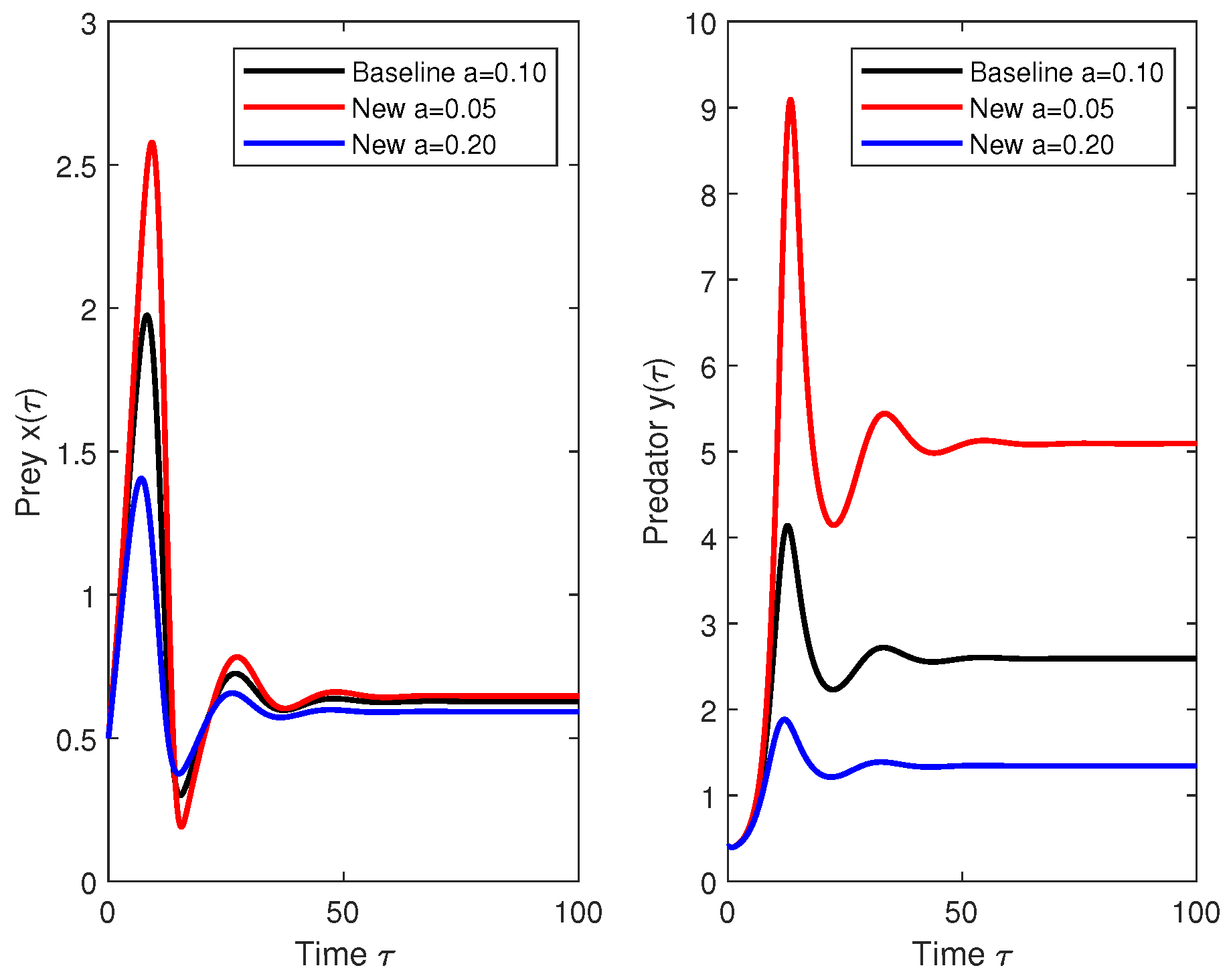
In Figure 2, Figure 3, Figure 4 and Figure 5, we used the baseline values $r=0.1$, $a=0.1$, $b=0.3$, and $m=0.2$ and then varied each parameter one at a time while keeping others fixed. The baseline values of the parameters are selected based on the values reported in [23]. The original predator–prey model without delays was considered in [23].

Figure 2. Prey and predator dynamics with r variation.

Figure 3. Prey and predator dynamics with a variation.

Figure 4. Prey and predator dynamics with b variation.

Figure 5. Prey and predator dynamics with m variation.

1: Varying Prey Growth r. For a small value of r, i.e., 0.05, the prey population grows slowly, which limits predator availability. The predator density declines earlier and stabilizes at a lower level. For the baseline value of r, i.e., 0.1, both populations oscillate with moderate amplitudes before reaching equilibrium. For a large r, i.e., 0.2, faster prey replenishment initially boosts predator density, but strong oscillations appear. The system takes longer to stabilize, showing possible persistence of predator–prey cycles.

2: Varying Predation Rate a. In the case of a small a, i.e., 0.05, the predators catch fewer prey; thus, prey density grows unchecked while predators stabilize at very low values. In case of baseline $a=0.1$, a balanced predation maintains both species in coexistence with oscillatory adjustment. For a large a, i.e., 0.2, strong predation reduces prey drastically. Predator density initially increases but then suffers due to prey scarcity, leading to dampened oscillations and possible predator decline. Thus, too high predation destabilizes prey survival; too low predation risks predator extinction.

3: Varying Predator Conversion Efficiency b. For a small value of b, i.e., 0.2, the predators inefficiently convert prey into reproduction. Despite prey abundance, predator growth is weak, leading to predator decline. For baseline $b=0.3$, a balanced coexistence with moderate oscillations is observed. For a large value of b, i.e., 0.5, the predators convert prey into reproduction very efficiently, leading to predator dominance. However, prey depletion follows, resulting in oscillations of high amplitude. Thus, higher conversion efficiency strengthens predator dominance but risks prey extinction.

4: Varying Predator Mortality m. For a small value of m, i.e., 0.1, the predator mortality is low, so predators persist strongly, keeping prey at lower levels. For a baseline value of m, i.e., 0.2, a balanced coexistence is observed. For a large value of m, i.e., 0.3, the predators die faster, leading to weaker predator persistence. Prey recover more quickly, with predator density approaching near extinction in some runs. Thus, predator survival strongly depends on m. High mortality favors prey persistence but risks predator extinction.

In Figure 6 and Figure 7, we present predator and prey dynamics with varying fractional order.

Figure 6. Predator dynamics with variation of fractional order $\eta$.

Figure 7. Prey dynamics with variation of fractional order $\eta$.

In Figure 8 and Figure 9, we present predator and prey dynamics with varying fractal dimension.

Figure 8. Predator dynamics with variation of fractal dimension $\lambda$.

Figure 9. Prey dynamics with variation of fractal dimension $\lambda$.

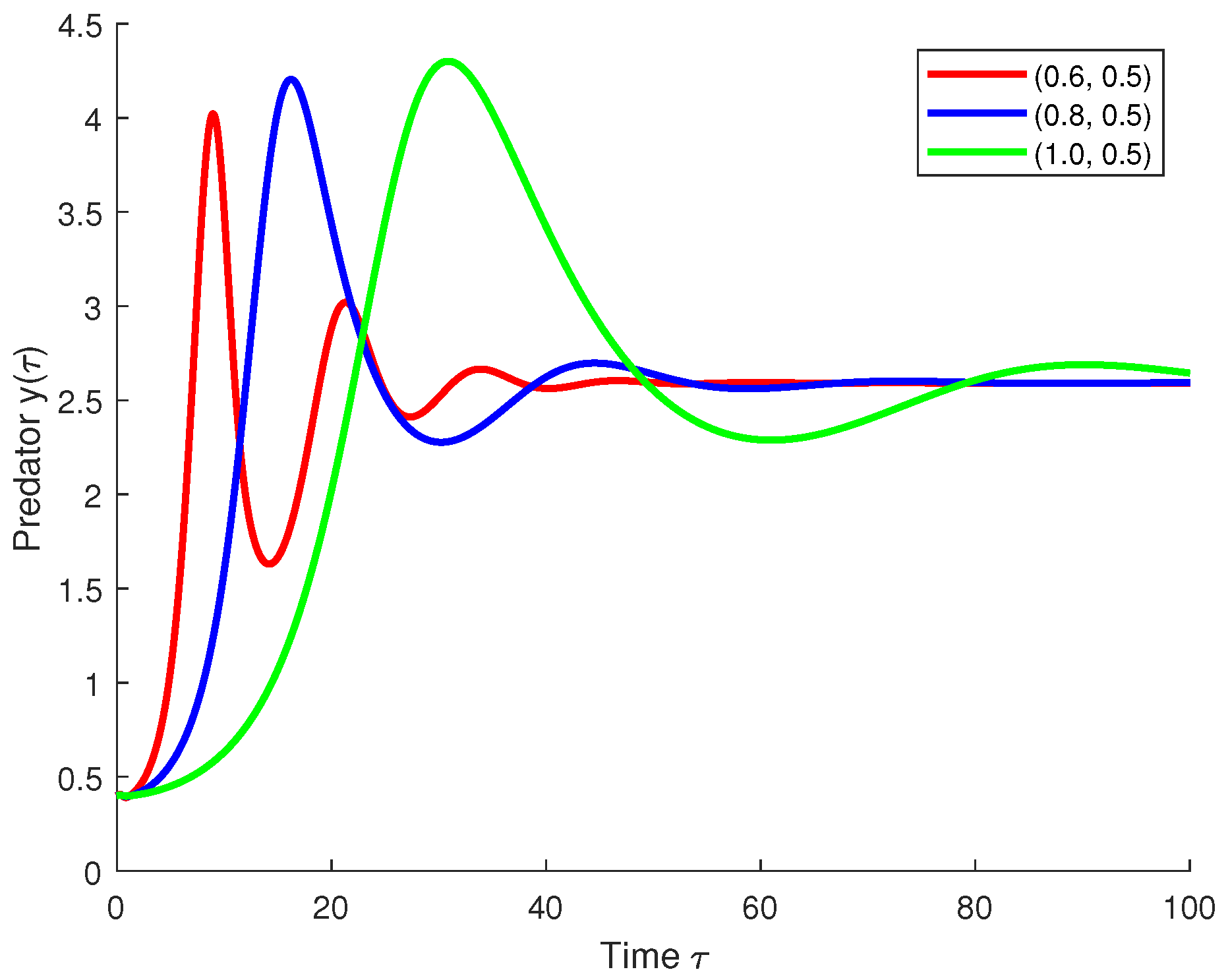
In Figure 6, we see that for $\eta =0.6$, the predator grows rapidly, overshoots early, and oscillations are frequent with higher amplitude initially, but dampen relatively quickly. For $\eta =0.8$, Predator oscillations are smoother, and dampening occurs faster than $\eta =0.6$. For $\eta =1.0$, the predator shows a slower rise and larger peak, and the oscillations are wider but settle later.

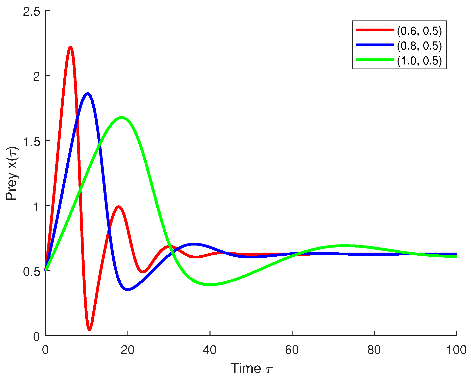
In Figure 7, it is observed that for $\eta =0.6$, prey shows sharp oscillations, including an initial dip below its starting level, then damps quickly. For $\eta =0.8$, oscillations are smoother and decay faster. For $\eta =1.0$, oscillations are broader, with slower dampening, and prey remains suppressed longer.

In Figure 8, it is observed that all three curves start with similar growth; however, the amplitude and timing of peaks are different. For $\lambda =0.5$, the predator attains the highest and most delayed peak. For $\lambda =0.7$, there is an earlier peak, slightly dampened. For $\lambda =0.9$, there is an even earlier rise and faster decay of the oscillations. This shows that increasing the fractal dimension accelerates stabilization and reduces predator overshoot. Similarly, a larger fractal dimension implies a stronger memory effect smoothing and dampening predator oscillations. Moreover, all curves stabilize to the same equilibrium.

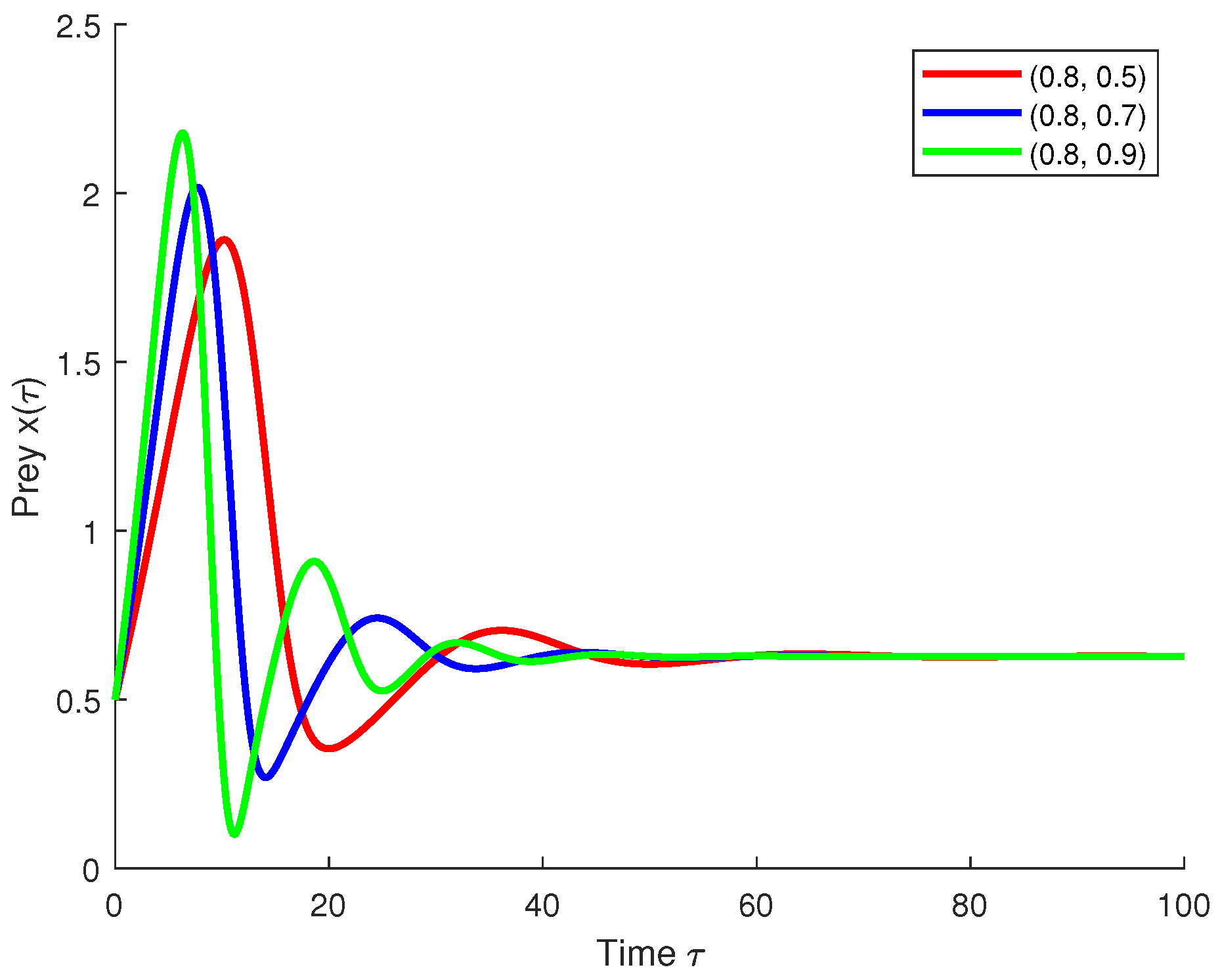
In Figure 9, it is observed that as the value of fractal dimension increases, the prey dynamics exhibit relatively higher frequencies and amplitudes.

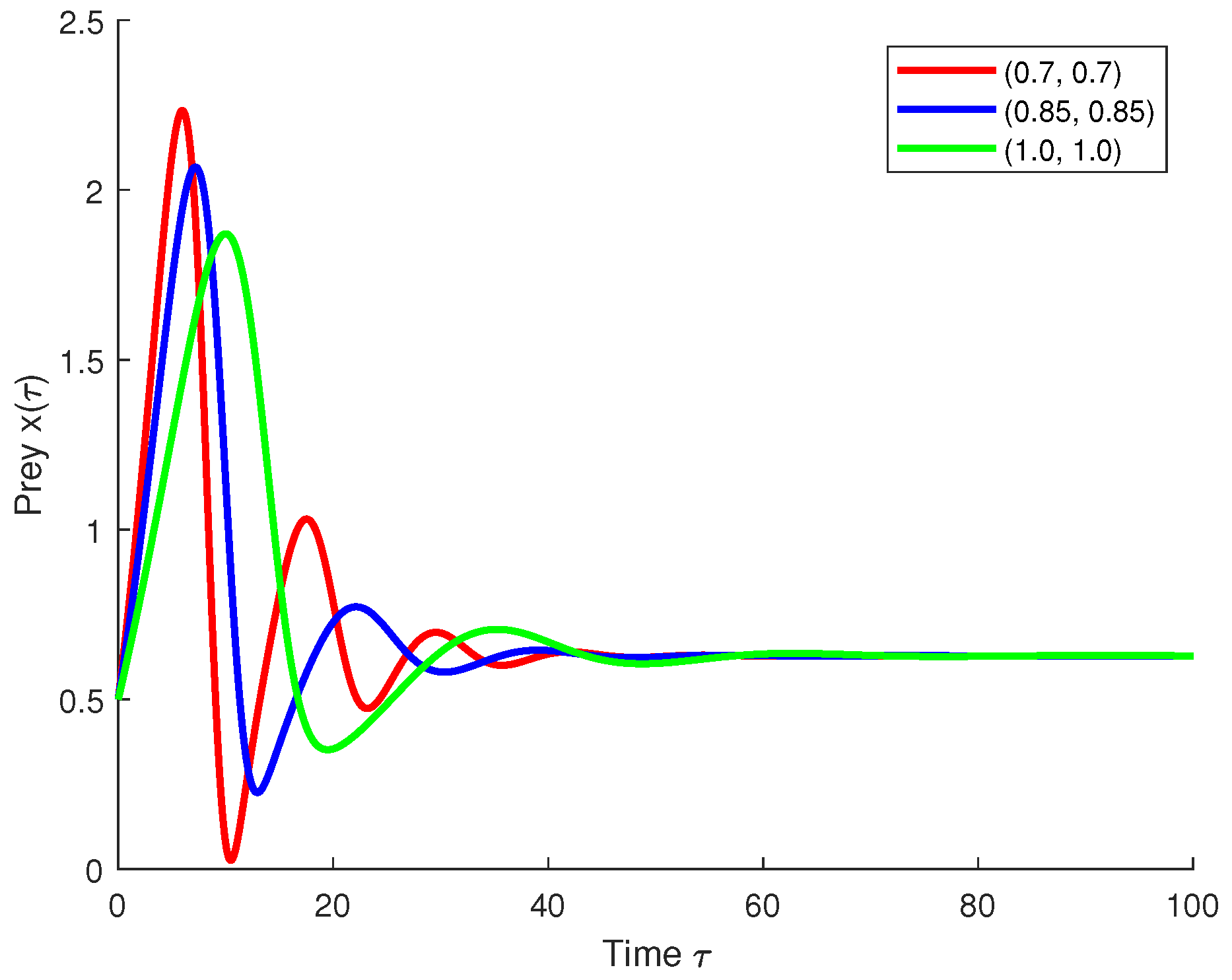
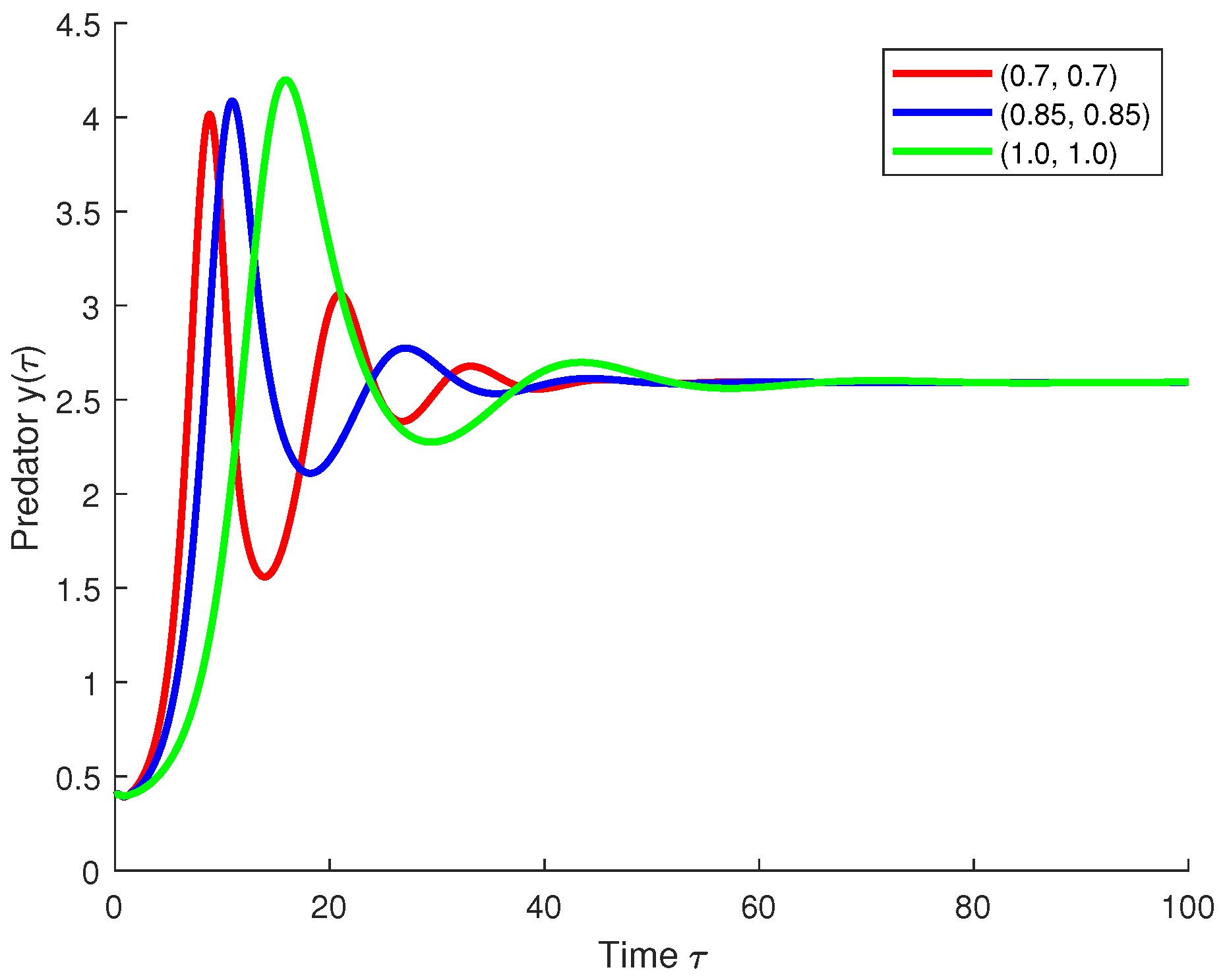
In Figure 10 and Figure 11, we present predator and prey dynamics with both varying fractional order and both having the same values for fractal dimension.

Figure 10. Dynamics of predator–prey model under different fractional order $\eta$ and fractal dimension $\lambda$.

Figure 11. Predator dynamics of predator–prey model under different fractional order $\eta$ and fractal dimension $\lambda$.

From Figure 10, the prey population dynamics demonstrate notable sensitivity to changes in the fractional and fractal order parameters $(\eta ,\lambda )$. For lower values (such as $\eta =\lambda =0.7$), the prey species exhibits pronounced oscillatory patterns with relatively higher frequencies and amplitudes. This suggests that in environments where memory effects are stronger (i.e., the system “remembers” its past behavior more heavily), prey populations may undergo rapid cycles due to delayed responses to predation and growth. As the order increases towards $\eta =\lambda =1.0$, which corresponds to the classical (non-fractional) case, the oscillations become smoother and less intense, indicating that memory effects contribute significantly to the emergence of irregular fluctuations in prey populations.

Interestingly, Figure 11 highlights a different dynamic for the predator species. Contrary to the prey, the predator population tends to exhibit dampened oscillations for lower-order values, while the amplitude of oscillations increases with higher $(\eta ,\lambda )$. This reversal in behavior can be attributed to the indirect dependence of predators on delayed prey information, as encoded in both constant and state-dependent delays. In fractional-order systems, the rate of change depends on the entire history of the system, not just its current state. Therefore, the predator’s access to past prey availability plays a crucial role in its population changes. At higher values of the fractional order, where memory effects are less dominant, the predator responds more sharply to fluctuations, leading to stronger oscillatory behavior.

These contrasting responses between prey and predator species under varying memory intensities emphasize the importance of incorporating fractional and fractal features into ecological modeling. Traditional integer-order models often fail to account for such nonlocal and history-dependent processes, potentially oversimplifying the complex feedback mechanisms in biological systems. The present model demonstrates that fractional calculus not only adds realism but also allows us to explore parameter regimes where classical models may not be valid or stable.

Overall, the findings suggest that fractional-order modeling provides a flexible framework to study the impact of memory, delays, and structural complexity in coupled systems. This opens up new avenues for designing more accurate predictive models in ecology, epidemiology, and neuroscience, where time lags and hereditary effects are fundamental to system dynamics.

6. Conclusions

This research formulated and analyzed a coupled system of fractal–fractional Caputo differential equations incorporating both constant and state-dependent delay effects. The model more accurately captures adaptive delay dynamics encountered in real-world systems such as neural feedback loops and population interactions. We provided sufficient assumptions under which at least one solution exists and is unique. Also, we analyzed the HU stability of the model. We applied our proposed model to two numerical problems, including a real-world predator–prey model, and simulated its dynamics. The numerical simulations conducted reveal insightful characteristics about the interaction dynamics under different memory effects. The inclusion of both constant and state-dependent delays, in conjunction with the fractal–fractional Caputo-type operator, allows the model to capture nonlocal effects and hereditary behavior that are commonly present in ecological systems. These results extend the theory of delay differential systems in the context of generalized fractional calculus and offer a mathematically rich platform for future analytical and numerical exploration. The parameter values used in the numerical example are illustrative and follow typical magnitudes employed in predator–prey studies [23]. They are not fitted to empirical data but chosen to demonstrate qualitative behavior under fractal–fractional dynamics. Incorporating real ecological datasets is an interesting direction for future work.

References

- Cushing, J.M. Integrodifferential Equations and Delay Models in Population Dynamics; Springer: Berlin, Germany, 2013. [Google Scholar]
- MacDonald, N. Time Lags in Biological Models; Lecture Notes in Biomathematics; Springer: Heidelberg, Germany, 1978; Volume 27. [Google Scholar]
- Gopalsamy, K. Stability and Oscillations in Delay Differential Equations of Population Dynamics; Springer: Berlin, Germany, 2013. [Google Scholar]
- Kuang, Y. Delay Differential Equations with Applications in Population Dynamics; Academic Press: New York, NY, USA, 1993. [Google Scholar]
- Lin, X.; Wang, H. Stability analysis of delay differential equations with two discrete delays. Can. Appl. Math. Q. 2012, 20, 519–533. [Google Scholar]
- Xu, C.; Liao, M.; Li, P.; Guo, Y. Bifurcation analysis for simplified five-neuron bidirectional associative memory neural networks with four delays. Neural Process. Lett. 2019, 50, 2219–2245. [Google Scholar] [CrossRef]
- Shah, K.; Sher, M.; Sarwar, M.; Abdeljawad, T. Analysis of a nonlinear problem involving discrete and proportional delay with application to houseflies model. AIMS Math. 2024, 9, 7321–7339. [Google Scholar] [CrossRef]
- Bellen, A.; Zennaro, M. Numerical Methods for Delay Differential Equations; Numerical Mathematics and Scientific Computation Series; Oxford University Press: Oxford, UK, 2003. [Google Scholar]
- Ruan, S. Delay differential equations in single species dynamics. In Delay Differential Equations and Applications; Arino, O., Hbid, M.L., Dads, E.A., Eds.; Springer: Dordrecht, The Netherlands, 2006; pp. 477–517. [Google Scholar] [CrossRef]
- Rihan, F.A. Delay Differential Equations and Applications to Biology; Springer: Singapore, 2021. [Google Scholar]
- Cooke, K.L.; Yorke, J.A. Some equations modelling growth processes and gonorrhea epidemics. Math. Biosci. 1973, 16, 75–101. [Google Scholar] [CrossRef]
- Beuter, A.; Bélair, J.; Labrie, C.; Bélair, J. Feedback and delays in neurological diseases: A modeling study using dynamical systems. Bull. Math. Biol. 1993, 55, 525–541. [Google Scholar] [CrossRef]
- Bélair, J.; Mackey, M.C.; Mahaffy, J.M. Age-structured and two-delay models for erythropoiesis. Math. Biosci. 1995, 128, 317–346. [Google Scholar] [CrossRef]
- Mahaffy, J.M.; Joiner, K.M.; Zak, P.J. A geometric analysis of stability regions for a linear differential equation with two delays. Int. J. Bifurc. Chaos 1995, 5, 779–796. [Google Scholar] [CrossRef]
- Podlubny, I. Fractional Differential Equations; Academic Press: San Diego, CA, USA, 1999. [Google Scholar]
- Samko, S.G.; Kilbas, A.A.; Marichev, O.I. Fractional Integrals and Derivatives: Theory and Applications; Gordon and Breach: North Holland, The Netherlands, 1993. [Google Scholar]
- Alazopoulos, K.A. Non-local continuum mechanics and fractional calculus. Mech. Res. Commun. 2006, 33, 753–757. [Google Scholar] [CrossRef]
- Atangana, A. Fractal-fractional differentiation and integration: Connecting fractal calculus and fractional calculus to predict complex systems. Chaos Solitons Fractals 2017, 102, 396–406. [Google Scholar] [CrossRef]
- Aldwoah, K.A.; Almalahi, M.A.; Hleili, M.; Alqarni, F.A.; Aly, E.S.; Shah, K. Analytical study of a modified-ABC fractional order breast cancer model. J. Appl. Math. Comput. 2024, 70, 3685–3716. [Google Scholar] [CrossRef]
- Khan, H.; Alzabut, J.; Shah, A.; He, Z.; Etemad, S.; Rezapour, S.; Zada, A. On fractal-fractional waterborne disease model: A study on theoretical and numerical aspects of solutions via simulations. Fractals 2023, 31, 2340055. [Google Scholar] [CrossRef]
- Hamza, A.E.; Osman, O.; Ali, A.; Alsulami, A.; Aldwoah, K.; Mustafa, A.; Saber, H. Fractal-fractional-order modeling of liver fibrosis disease and its mathematical results with subinterval transitions. Fractal Fract. 2024, 8, 638. [Google Scholar] [CrossRef]
- Alraqad, T.; Almalahi, M.A.; Mohammed, N.; Alahmade, A.; Aldwoah, K.A. Modeling Ebola dynamics with a Φ-piecewise hybrid fractional derivative approach. Fractal Fract. 2024, 8, 596. [Google Scholar] [CrossRef]
- Tahara, T.; Gavina, M.K.A.; Kawano, T.; Tubay, J.M.; Rabajante, J.F.; Ito, H. Asymptotic stability of a modified Lotka-Volterra model with small immigrations. Sci. Rep. 2018, 8, 13894. [Google Scholar] [CrossRef]
- Yang, W. Positive solutions for a coupled system of nonlinear fractional differential equations with integral boundary conditions. Comput. Math. Appl. 2012, 63, 288–297. [Google Scholar] [CrossRef]
- Li, M.; Liu, Y. Existence and uniqueness of positive solutions for a coupled system of nonlinear fractional differential equations. Open J. Appl. Sci. 2013, 3, 53–61. [Google Scholar] [CrossRef]
- Houas, M.; Dahmani, Z. New results for a coupled system of fractional differential equations. Facta Univ. Ser. Math. Inform. 2013, 28, 133–150. [Google Scholar]
- Ali, A.; Bibi, F.; Ali, Z.; Shah, K.; Abdalla, B.; Abdeljawad, T. Investigation of existence and Ulam’s type stability for coupled fractal fractional differential equations. Eur. J. Pure Appl. Math. 2025, 18, 5963. [Google Scholar] [CrossRef]
- Younis, M.; Öztürk, M. Some novel proximal point results and applications. Univers. J. Math. Appl. 2025, 8, 8–20. [Google Scholar] [CrossRef]
- Abdou, A.A.N. Solving a nonlinear fractional differential equation using fixed point results in orthogonal metric spaces. Fractal Fract. 2023, 7, 817. [Google Scholar] [CrossRef]
- Alqahtani, B.; Fulga, A.; Karapinar, E. Common fixed point results on an extended b-metric space. J. Inequal. Appl. 2018, 2018, 158. [Google Scholar] [CrossRef]
- Hetmaniok, E.; Pleszczyński, M.; Khan, Y. Solving the integral differential equations with delayed argument by using the DTM method. Sensors 2022, 22, 4124. [Google Scholar] [CrossRef]
- Schaefer, H. Über die Methode der a Priori-Schranken. Math. Ann. 1955, 129, 415–416. [Google Scholar] [CrossRef]
- Rus, I.A. Ulam stabilities of ordinary differential equations in a Banach space. Carpath. J. Math. 2010, 26, 103–107. [Google Scholar]
- Khan, M.A.; Atangana, A. Numerical Methods for Fractal-Fractional Differential Equations and Engineering Simulations and Modeling; CRC Press: Boca Raton, FL, USA, 2023. [Google Scholar]
- Marsudi, I.; Darti, A. A comparative study on numerical solutions of initial value problems of differential equations using three numerical methods. BAREKENG J. Math. Appl. 2025, 19, 1263–1278. [Google Scholar] [CrossRef]
Disclaimer/Publisher’s Note: The statements, opinions and data contained in all publications are solely those of the individual author(s) and contributor(s) and not of MDPI and/or the editor(s). MDPI and/or the editor(s) disclaim responsibility for any injury to people or property resulting from any ideas, methods, instructions or products referred to in the content. |
© 2025 by the authors. Licensee MDPI, Basel, Switzerland. This article is an open access article distributed under the terms and conditions of the Creative Commons Attribution (CC BY) license (https://creativecommons.org/licenses/by/4.0/).