Research on Slope Early Warning and Displacement Prediction Based on Multifractal Characterization

Abstract

The occurrence of landslide hazards significantly induces changes in slope surface displacement. This study conducts an in-depth analysis of the multifractal characteristics and displacement prediction of highway slope surface displacement sequences. Utilizing automated monitoring devices, data are collected to analyze the deformation patterns of the slope surface layer. Specifically, the multifractal detrended fluctuation analysis (MF-DFA) method is employed to examine the multifractal features of the monitoring data for slope surface displacement. Additionally, the Mann–Kendall (M-K) method is combined to construct the α indicator and $f\left(\alpha \right)$ indicator criteria, which provide early warnings for slope stability. Furthermore, the long short-term memory (LSTM) model is optimized using the particle swarm optimization (PSO) algorithm to enhance the prediction of slope surface displacement. The results indicate that the slope displacement monitoring data exhibit a distinct fractal sequence characterized by $h\left(q\right)$, with values decreasing as the fluctuation function q decreases. Through this study, the slope landslide warning classification has been determined to be Level III. Moreover, the PSO-LSTM model demonstrates superior prediction accuracy and stability in slope displacement forecasting, achieving a root mean square error (RMSE) of 0.72 and a coefficient of determination (R²) of 91%. Finally, a joint response synthesis of the slope landslide warning levels and slope displacement predictions resulted in conclusions. Subsequent surface displacements of the slope are likely to stabilize, indicating the need for routine monitoring and inspection of the site.

1. Introduction

With the continuous development of transportation infrastructure in China, a significant number of highways, railroads, and other projects have been established. Due to the terrain, many highway and railroad projects must traverse mountainous areas, making slope engineering crucial in the construction of high-speed infrastructure in these regions [1,2]. Slopes are common structures in geotechnical engineering, and their stability is influenced by numerous factors characterized by randomness, ambiguity, and uncertainty [3,4,5,6,7]. In recent years, the growth of highway transportation, mining, and related industries in China has heightened the demand for slope engineering, leading to an increase in slope failure incidents. This trend poses safety risks to the public and generates substantial economic losses for the country [8,9,10,11,12,13,14]. Consequently, accurately determining the slope warning level is a critical issue in geotechnical engineering.

During the service life of slope engineering, monitoring and controlling surface displacement is a key technological challenge. As such, the evaluation of slope surface displacement stability is particularly important. Current methods for slope stability analysis include numerical simulation techniques [15,16,17,18,19,20], cluster analysis [21,22,23,24,25,26,27], image recognition [28,29,30,31], and machine learning approaches [32,33,34,35,36,37]. However, due to the complexity of the geological environment and various deformation-inducing factors. This leads to the time-series curve of slope surface displacement showing obvious volatility and strong nonlinear characteristics. Thus, multifractal detrended fluctuation analysis (MF-DFA) provides an effective tool for analyzing tunnel deformation.

Analyzing the deformation patterns in slope monitoring data offers technical support and theoretical guidance for early warning systems, which is vital for enhancing slope safety. For instance, Yuanfeng Dong et al. [38] investigated the Chongqing Tongnan orchard landslide, analyzing various monitoring results to grade the landslide warning levels accurately and issue critical slip warnings, thereby preventing property damage and casualties. Similarly, Xiaopeng Deng [39] utilized cusp catastrophe theory to evaluate the stability of the Bazimen landslide in the Three Gorges Reservoir area, achieving a comprehensive assessment of landslide warning through limit displacement criteria and V/S analysis. Shuang Zhou et al. [40] employed an intensity reduction finite difference calculation approach, combined with monitoring data, but did not achieve effective slope deformation warnings. While previous studies have explored early warning mechanisms for slopes, they often overlooked the investigation of multifractal characteristics. In contrast, Heng Lei et al. [41] and Haoyu Mao et al. [42] applied multifractal theory to slope deformation warnings, successfully revealing warning signals through displacement data and micro-seismic signal monitoring, demonstrating the potential of this theory in early warning applications. Thus, further exploration of multifractal characteristics, based on slope surface displacement monitoring data and evaluation of early warning classifications, remains a valuable avenue for research.

Accurate prediction of slope deformation is also crucial for disaster prevention and warning systems. Machine learning methods have been increasingly employed for slope deformation prediction. Long short-term memory (LSTM) networks are proven to be particularly effective due to their ability to capture long-term dependencies and process temporal information [43]. Jiangbo Xu et al. [44] developed an LSTM model for slope displacement prediction, leveraging the maximum mutual information coefficient and the XGBoost algorithm, ultimately concluding that the model demonstrates high reliability. Haiping Xiao et al. [45] proposed a slope deformation prediction model integrating genetic algorithms and LSTM, achieving high accuracy and stability. Moreover, swarm intelligence optimization algorithms, such as particle swarm optimization (PSO), can enhance PSO-LSTM performance, leading to recent applications of the LSTM model in slope deformation prediction. Therefore, further application of the PSO-LSTM model for predicting slope displacements is warranted.

The study of disaster early warning is of paramount importance for disaster prevention and mitigation. With advancements in science and technology, monitoring and early warning systems have emerged as crucial tools for the proactive prevention of geological disasters. Currently, the LSTM models [46,47,48,49,50] and MF-DFA methods [51,52,53,54,55] have been widely applied in numerous studies focused on early warning for geological disasters. By utilizing a real-time monitoring and warning model for landslides, we can achieve dynamic tracking and timely alerts. Based on the grading results of landslide disaster early warnings, rapid decision-making and appropriate emergency measures can be implemented. This approach effectively reduces casualties and property losses associated with landslide disasters.

Building on these findings, research into the early warning predictions of slope landslides is essential. This paper utilizes monitoring data of slope surface displacement to first conduct a MF-DFA and Mann–Kendall (M-K) analysis, focusing on the multifractal features and early warning classifications of slope landslides. Subsequently, PSO-LSTM is employed to predict slope surface displacement data, forecasting displacement for the next 112 h. Finally, the results from the multifractal analysis and displacement predictions are combined to comprehensively evaluate the warning level of slope deformation, providing essential theoretical guidance for practical slope management.

2. Materials and Methods

2.1. Projiect Overview and Monitoring Data

This study focuses on a slope located within the Keqiao to Zhuji Expressway Project, specifically in the bidding section TJ03. This contract section spans Diankou Town and Yaojiang Town in Zhuji City, Shaoxing District. The slope begins in the middle of Keqiao, extends southwest through the southern part of Diankou, and terminates in the northern region of Zhuji City. The topography of the area is characterized by a low elevation at both ends and a higher elevation in the middle, resulting in a varied landscape.

The slope is part of a hilly terrain, where the section under investigation is an open quarry. Excavation is clearly defined, revealing medium weathering bedrock with exposed characteristics. At the summit of the slope, there exists a thin layer of residual slope deposits containing gravel and powdery clay. The underlying bedrock consists of Aurignacian Zhitang group tuff sandstone, which exhibits significant joint fissures and a broken rock structure.

The slope extends from K20 + 415 to K20 + 510, measuring a total length of 111 m, with a maximum height of 31.3 m. On the left flank of the K20 + 460 section, the slope is constructed in three tiers, each with a gradient of 1:2, where the third tier is excavated directly to the top, achieving a maximum excavation height of 30 m. Conversely, the right side of the slope is excavated with a gradient of 1:1.5, reaching a maximum height of 4 m. The overall slope configuration is step-like, with each tier height measuring 10 m and a 2-m-wide crumbling platform situated between each tier. Following the completion of the excavation, the slope configuration is illustrated in Figure 1a.

To ensure the safety and stability of the slope post-excavation, an automatic monitoring system has been installed. This system monitors surface displacements of the slope at a frequency of once every 8 h to collect data, as depicted in Figure 1b.

To accurately assess the stability of the slope, continuous monitoring of surface displacement is conducted. Initially, the monitoring area and the locations of appropriate monitoring points are established. The safety conditions of the slope are evaluated based on the collected monitoring data. In this study, a total of 440 sets of slope monitoring data, collected from 29 January 2024 to 24 June 2024, are analyzed. The data from the monitoring points are compiled to generate the slope displacement–time diagram, as illustrated in Figure 2.

2.2. MF-DFA

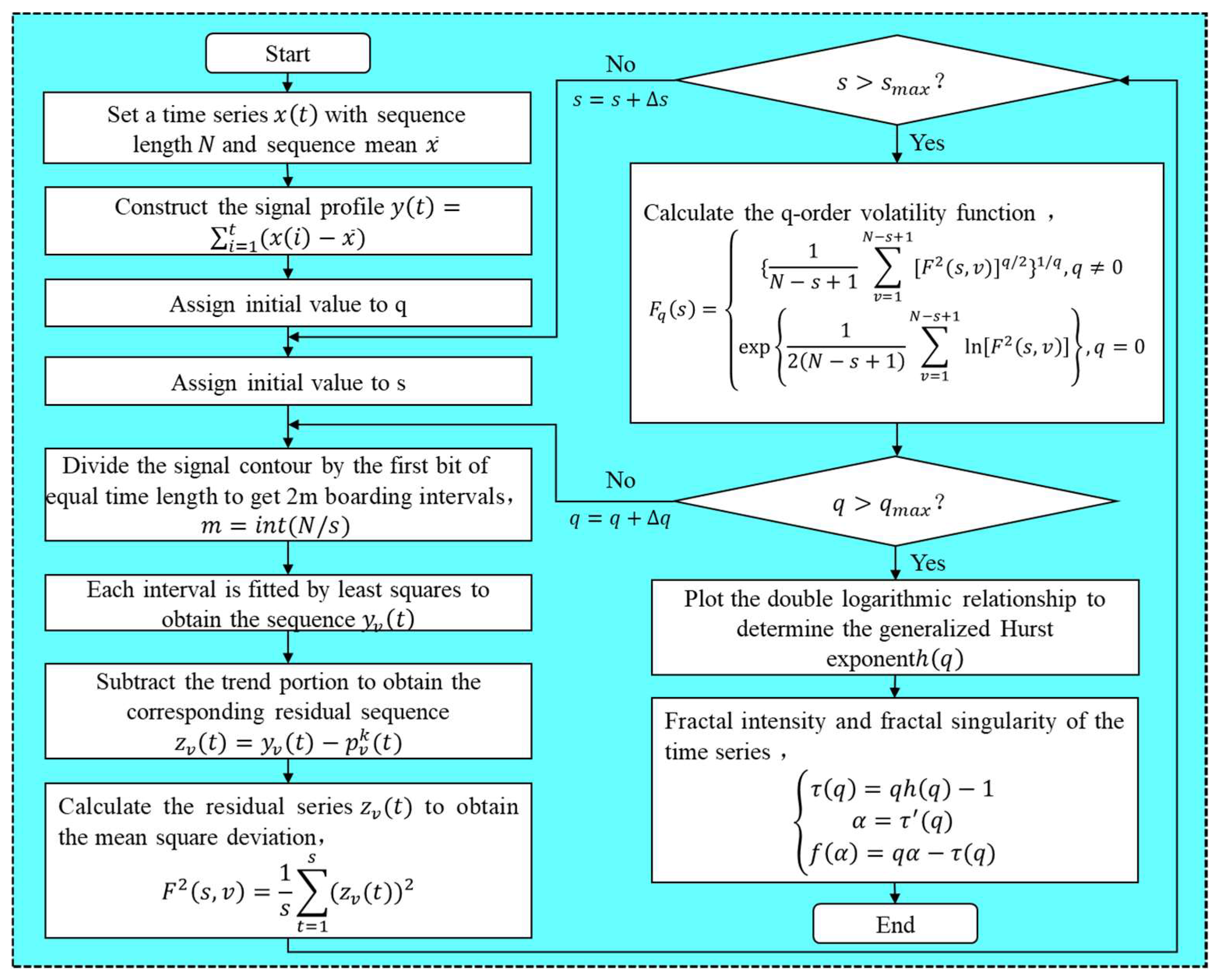
In the contexts of stochastic processes, chaos theory, and time series analysis, detrended fluctuation analysis (DFA) serves as a method for calculating the $\alpha$ (or Hurst exponent) to assess the statistical self-similarity of a signal. However, traditional DFA computes only second-order statistical moments and assumes that the underlying process follows a normal distribution. In contrast, the MF-DFA evaluates all $q$-order statistical moments $h\left(q\right)$, providing a more comprehensive characterization of nonlinear data and non-smooth signals compared to traditional DFA. The calculation flow for MF-DFA is illustrated in Figure 3.

2.3. M-K Test Method

The M-K test method is a non-parametric method. The specific calculation steps are as follows:

Step 1: There is a sample size of $\left\{x_1,x_2,\dots \dots ,x_n\right\}$ of time series. For all the $k$($j\le n$ and $k\ne j$), the distributions of $x_k$ and $x_j$ are different, and the difference function $Sgn\left(x_j-x_k\right)$ is computed:

$$Sgn\left(x_j-x_k\right)=\left\{\begin{array}{c}+1, \left(x_j-x_k\right)>0\\ 0, \left(x_j-x_k\right)=0\\ -1, \left(x_j-x_k\right)<0\end{array}\right.$$

(1)

Step 2: Calculate the test statistic $S$:

$$S=\sum _{k=1}^{n-1}\sum _{j=k+1}^{n}Sgn(x_j-x_k)$$

(2)

Step 3: $S$ is normally distributed with mean 0. Calculate the variance $Var\left(S\right)$:

$$Var\left(s\right)={\displaystyle \frac{n(n-1)(2n+5)}{18}}$$

(3)

Step 4: Calculate the standard normal statistical variable $Z$:

$$Z=\left\{\begin{array}{c}{\displaystyle \frac{S-1}{\sqrt{Var\left(s\right)}}}, S>0\\ 0, S=0\\ {\displaystyle \frac{S+1}{\sqrt{Var\left(s\right)}}}, S<0\end{array}\right.$$

(4)

Step 5: The trend characteristics of the evaluation object can be determined by the magnitude of $Z$. The $Z_{\alpha }$ value represents the critical threshold at the specified significance level $\alpha$. In this study, a significance test is conducted at a 99% confidence level, resulting in $\alpha =0.01$ and $Z_{0.01}=2.32$.

If $Z\ge Z_{\alpha }$, it indicates that the indicator criterion has a tendency to increase.

If $-Z_{\alpha }<Z<Z_{\alpha }$, it indicates that the indicator criterion has a smooth trend.

If $Z\le -Z_{\alpha }$, it indicates that the indicator criterion has a decreasing trend.

2.4. PSO-LSTM Prediction Modeling

2.4.1. LSTM

The primary advantage of LSTM models over other common machine learning algorithms lies in their unique “gate” structure. This structure allows the LSTM model to evaluate information based on the “memory” of the network. Information is selectively retained or discarded by multiplying by 1 or 0. The unitary state effectively solves the gradient vanishing problem associated with short-term memory by retaining sequence-relevant information throughout the sequence.

The gate structure employs a sigmoid activation function that compresses values between 0 and 1, which facilitates the updating of retained information while discarding less relevant data.

The LSTM model features three main gates:

• Forgetting Gate: This gate determines whether information should be discarded or retained. It processes relevant information through the sigmoid function, producing an output between 0 and 1, where values closer to 0 indicate less importance and greater likelihood of being discarded, while values closer to 1 signify critical information.
• Input Gate: This gate updates the cell state. After processing by both sigmoid and hyperbolic tangent ($tanh$) functions, a final output value closer to 0 indicates less importance, whereas a value closer to 1 indicates significant information.
• Output Gate: Similar to the input gate, the output gate determines the value of the next hidden state in the cell structure. The processed value from this gate is used to decide the information the hidden state should carry, which is then passed along with the new cell state.

$$f_t=\sigma (w_f\left[h_{t-1},x_t\right]+b_f)$$

(5)

$$i_t=\sigma (w_i\left[h_{t-1},x_t\right]+b_i)$$

(6)

$${\check{C}}_t=tanh(w_c\left[h_{t-1},x_t\right]+b_c)$$

(7)

$$C_t=f_t{C}_{t-1}+i_t{\check{C}}_t$$

(8)

$$o_t=\sigma (w_o\left[h_{t-1},x_t\right]+b_o)$$

(9)

$$h_t=O_{t}tanh{C}_t$$

(10)

$$tanhx=(e^x-e^{-x})/(e^x+e^{-x})$$

(11)

where $x$ represents the input vector, $h$ denotes the output vector, and $f$, $i$, and $o$ refer to the forgetting gate, input gate, and output gate, respectively. The variable $t$ indicates the time step. The activation functions $\sigma$ and $tanh$ are nonlinear. $C$ represents the cell state, while $w$ signifies the trainable weight matrix, and $b$ refers to the bias matrix.

2.4.2. Improvement of PSO Algorithm

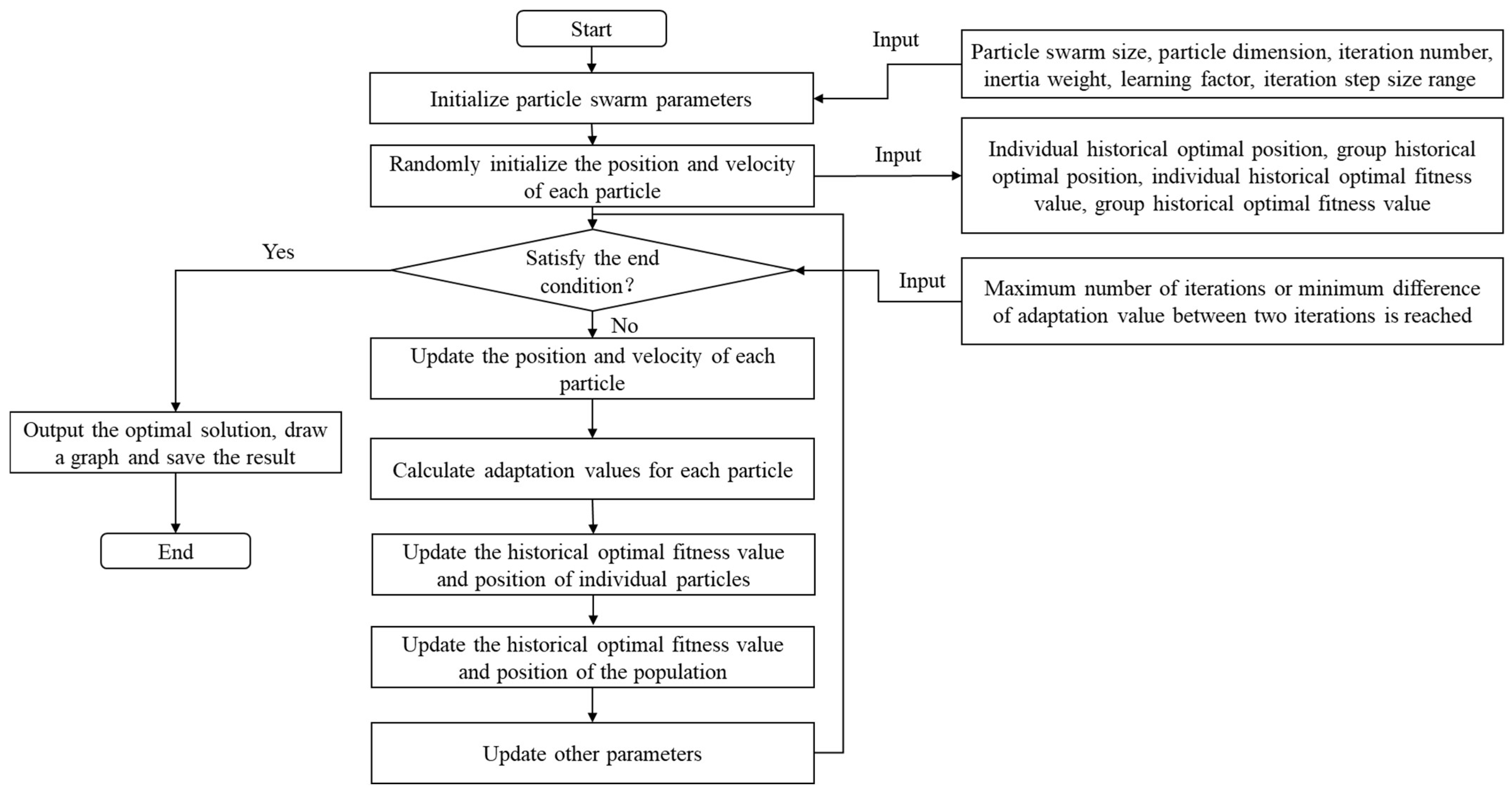
The PSO algorithm was developed by researchers inspired by the foraging behavior of birds. In this algorithm, each particle simulates the foraging behavior of a bird, with each particle in the swarm maintaining its own established direction while searching for the optimal value. Additionally, each particle communicates its current value and position to the swarm. Consequently, each particle adjusts its search direction based on its own experience as well as the position of the optimal value recorded by the swarm. The flow of the PSO algorithm is illustrated in Figure 4.

The mathematical expression for the base element of the PSO algorithm is

$$V_{id}^{k+1}=W{V}_{id}^k+C_1{r}_1\left(p_{id,pbest}^k-x_{id}^k\right)+C_2{r}_2\left(p_{id,gbest}^k-x_{id}^k\right)$$

(12)

$$x_{id}^{k+1}=x_{id}^k+V_{id}^{k+1}$$

(13)

where $V_{id}^{k+1}$ represents the $d$-dimensional component of the velocity of particle $i$ at the $k+1$ iteration; $W$ denotes the inertia weight; and $V_{id}^k$ is the d-dimensional component of the particle’s velocity at the $k$ iteration. $C_1$ and $C_2$ are the acceleration coefficients, while $r_1$ and $r_2$ are random numbers uniformly distributed between 0 and 1. $p_{id,pbest}^k$ indicates the d-dimensional component of particle $i$‘s historical optimal position at the $k$ iteration, and $x_{id}^k$ represents the position of the particle at the $k$ iteration. $p_{id,gbest}^k$ denotes the d-dimensional component of the optimal position recorded by the particle swarm throughout its history at the $k$ iteration. The term $C_1{r}_1$ represents the learning weight of the particle’s own experience, whereas $C_2{r}_2$ represents the learning weight based on the experiences of the population. Finally, $x_{id}^{k+1}$ is the $d$-dimensional component of the particle’s position at the $k+1$ iteration.

2.4.3. PSO-LSTM

The slope surface displacement data are input into the network structure of the LSTM model. Initially, the parameters of the LSTM model are established, followed by the initialization of particle swarm parameters. The positions and velocities of the particles are generated randomly, and the fitness values are computed. Subsequently, the individual and collective velocities and positions within the particle swarm are updated. After each update, the fitness values are recalculated to assess whether the maximum number of iterations has been reached. Upon reaching the maximum number of iterations, the optimal parameters are identified. The PSO-LSTM model is then constructed, and the data is both trained and tested, ultimately yielding the output results and evaluation metrics.

The coefficient of determination (R²), mean absolute error (MAE), and root mean square error (RMSE) were selected as evaluation criteria for the model. Their respective expressions are as follows:

$$\left\{\begin{array}{c}{R}^2=1-{\displaystyle \frac{{\sum }_{i=1}^n{[y_c\left(i\right)-y_0(i\left)\right]}^2}{{\sum }_{i=1}^n{[y_0\left(i\right)-\overline{y_c}]}^2}}\\ MAE={\displaystyle \frac{1}{n}}{\sum }_{i=1}^n\left|y_c\left(i\right)-y_0\left(i\right)\right|\\ RMSE=\sqrt{{\displaystyle \frac{1}{n}}{\sum }_{i=1}^n{[y_c\left(i\right)-y_0(i\left)\right]}^2}\end{array}\right.$$

(14)

where n represents the number of predicted outcomes. $y_o\left(i\right)$ represents the true outcome. $y_c\left(i\right)$ represents the predicted outcome. $\overline{y_o}$ represents the mean of the true values.

3. Results and Discussion

3.1. Multifractal Characterization of Slope Surface Displacement

Before calculating the multifractal characteristics of the monitoring data, it is essential to segment the data into four groups, each containing 110 data points. The groups are defined as follows: The first group spans from 29 January 2024 to 6 March 2024. The second group covers the period from 6 March 2024 to 11 April 2024. The third group extends from 12 April 2024 to 18 May 2024. The fourth group ranges from 18 May 2024 to 24 June 2024.

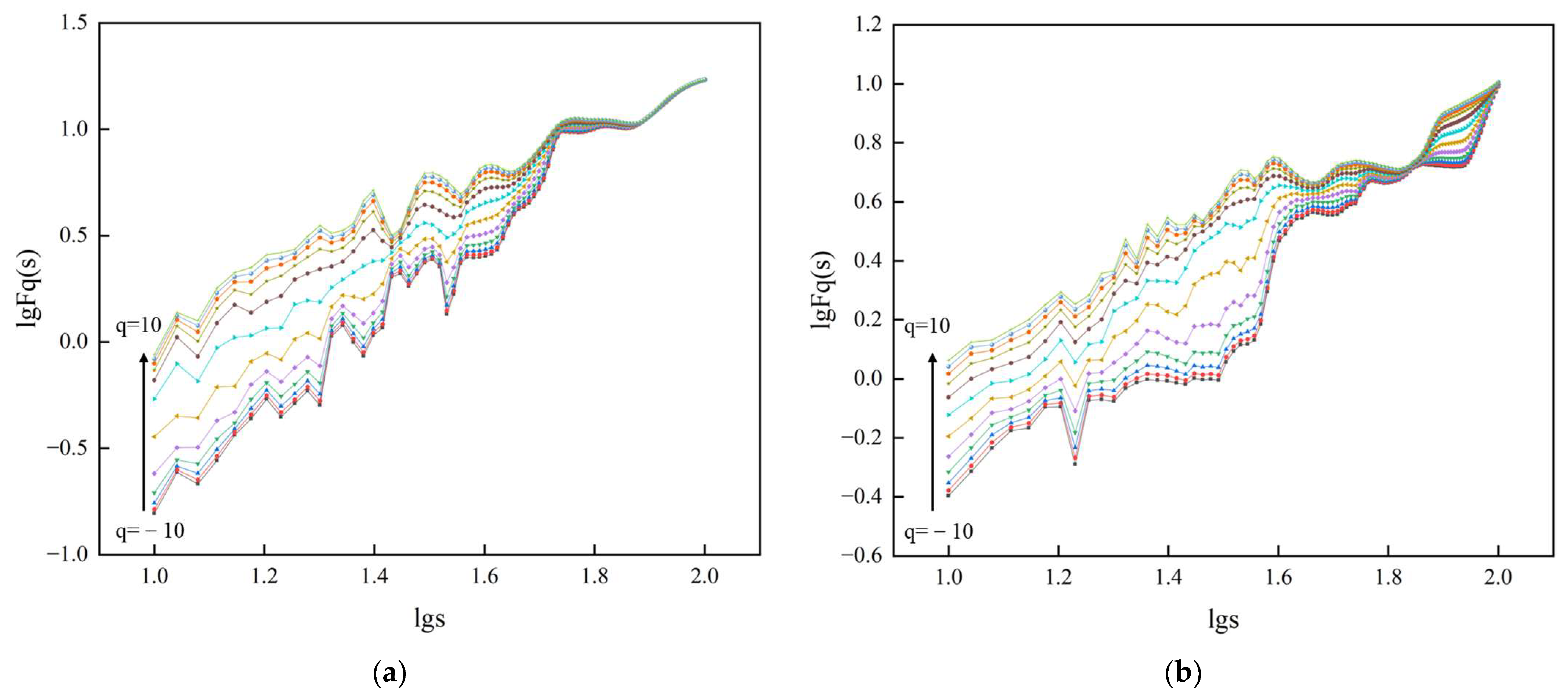
To perform multifractal analysis on each group of surface displacement monitoring sequences of the slope, we employed a sliding time window optimization method using the MF-DFA. In this analysis, the fluctuation order $q$ is varied over the range of [−10, 10], while the scale $s$ is set within the range of [10, 100]. The sliding window step is defined as 1. The resulting double logarithmic scatter plot of $log{F}_q\left(s\right)-logs$ is illustrated in Figure 5.

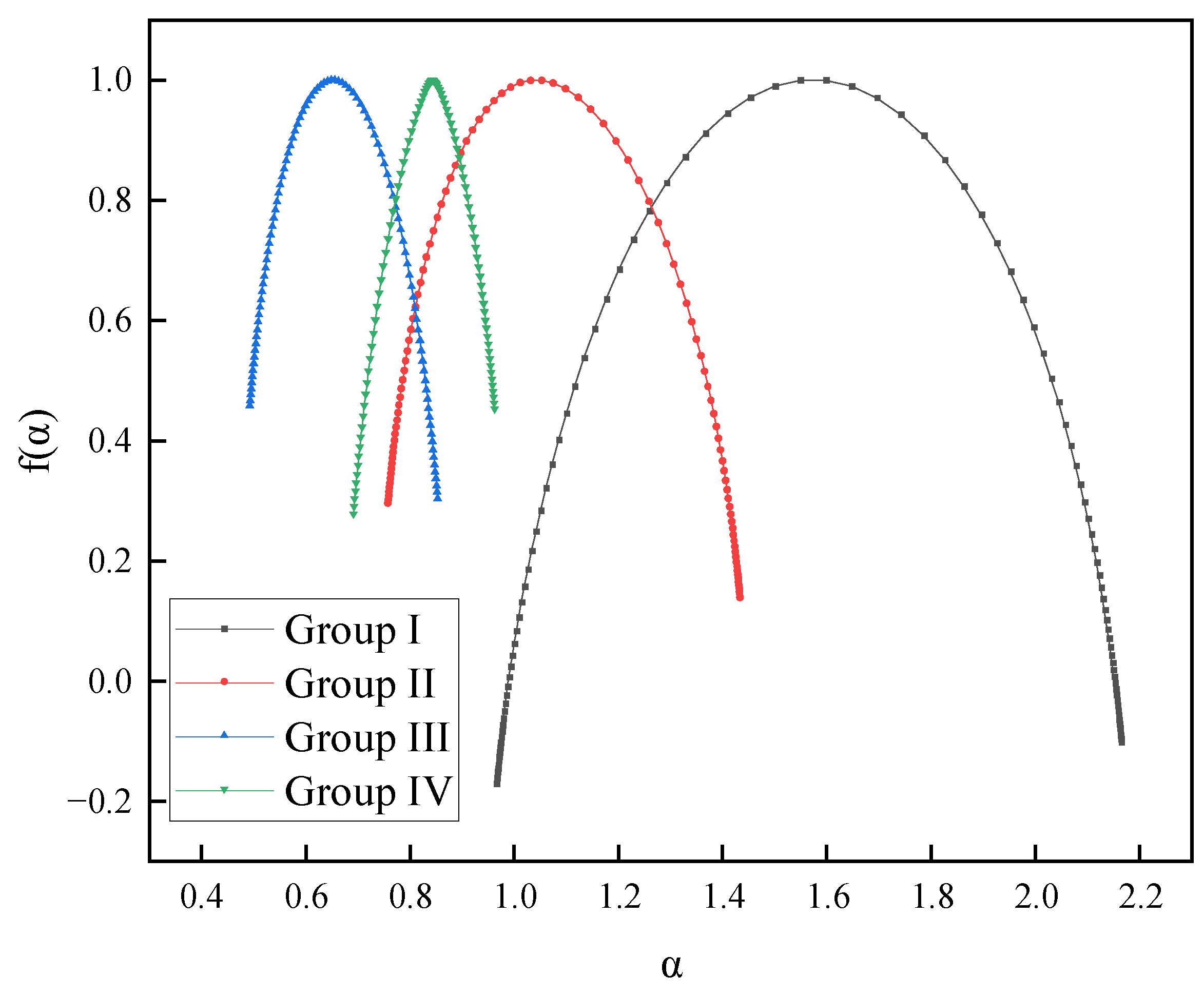
Using the aforementioned parameters, the four data series were analyzed through multifractal analysis with Matlab (R2018b) software. The generalized Hurst exponent and Renyi exponent—specifically, the scalar function—for each group of displacement sequences were computed across varying values of $\tau \left(q\right)$. The changes in the indices corresponding to the measurement point sequences are presented in Figure 6. Furthermore, the multifractal spectra for each group of displacement sequences are displayed in Figure 7.

As illustrated in Figure 6a, the generalized Hurst exponent of the surface displacement data series for the slope exhibits a nonlinear decreasing trend as $q$ varies within the range of [−10, 10]. This trend indicates that the surface displacement data at the monitoring sites is characterized by multifractal properties. Notably, for different fluctuation orders $q$, the generalized Hurst index curves of the second, third, and fourth groups are positioned at lower fluctuations compared to the first group, suggesting a weaker multifractal feature in these groups. However, the $h\left(q\right)$ values for each group’s displacement series are all greater than 0.5. Indicating that the displacement sequences possess strong memory and long-range correlations from the overall structure to local components.

Additionally, Figure 6b demonstrates a good consistency in the scale functions of the surface displacement sequences across all groups, with the central part of the scaling function curve exhibiting a convex shape that satisfies the relationship $\tau \left(0\right)=-1$. This finding further confirms that each group’s unique surface layer sequences exhibit multifractal characteristics.

As shown in Figure 7, the multifractal spectra for each group of slope surface displacement sequences exhibit a typical single-peak convex distribution, resembling a quadratic function curve. The local scales of these spectra vary, indicating the diversity of local variations across different time points. The singularity intensity α of most displacement sequences is distributed along both sides of the graph, reflecting the uneven distribution of the fractal structure within each data series. This further underscores the multifractal properties of the slope surface displacement sequences. Moreover, the multifractal spectral curves are generally symmetrical, suggesting a stable overall developmental state.

Utilizing Equation (8), we calculated the multifractal characteristic statistics for each group of surface displacement sequences. The results of these calculations are presented in

Table 1. Multifractal characterization statistics for surface displacements for each group of slopes.

Eigenvalue (Math.)	Group I	Group II	Group III	Group IV
$\Delta \alpha$	1.19744	0.67596	0.36077	0.2713
$\Delta f\left(\alpha \right)$	0.06878	−0.1566	−0.1539	0.17519

.

Table 1 reveals a comparison of the widths of the multifractal spectra for each group of displacement sequences, denoted as $\Delta \alpha$. The multifractal spectral width of the first group $\Delta \alpha$ is significantly greater than that of the other three groups, indicating that the multifractal intensity of the surface layer displacement sequences in the first group is higher, and the displacement fluctuations are more complex.

Furthermore, when comparing the proportions of large and small fluctuations ($\Delta f\left(\alpha \right)$) in the displacement series across each group, the fourth group shows a slightly higher $\Delta f\left(\alpha \right)$ compared to the other three groups. This suggests that the displacement sequences for the fourth group exhibit a greater prevalence of small fluctuations.

These findings indicate that the calculated multifractal eigenvalues of the surface displacement sequences are more consistent with actual monitoring results. Thus, the eigenvalues can be utilized for the study of landslide early warning grading in slopes.

3.2. Early Warning Grading Study of landslides on Slopes

3.2.1. Criteria for Classifying the Warning Level of Landslides on Slopes

Building upon the results of existing research on landslide warning levels, we utilized the surface displacement monitoring data for each group to construct warning criteria based on the $\Delta \alpha$ and $\Delta f\left(\alpha \right)$ parameters. This framework enables the classification of landslide warning levels into three categories: Level I, Level II, and Level III.

• Level I warnings indicate that slope deformation is trending in an extremely unfavorable direction, posing a significant risk of damage and serving as a precursor to imminent disaster. In this scenario, it is recommended to implement necessary disaster prevention and management measures, including evacuation and relocation, to mitigate potential losses.
• Level II warnings indicate that deformation is moving in an unfavorable direction, presenting a general risk of damage.
• Level III warnings suggest that deformation is trending towards stabilization.

The specific criteria for these warning levels are detailed in

Table 2. Criteria for classifying the warning level of landslides on slopes.

Warning Level	$\Delta \mathit{\alpha }$ Indicator Criterion	$\Delta \mathit{f}\left(\mathit{\alpha }\right)$ Indicator Criterion	Treatment Measures
I	Decreasing trend	Increasing trend	Suspend construction and carry out necessary disaster prevention and management or relocation to avoid disaster damage.
II	Increasing trend	Decreasing trend	Enhance the frequency of monitoring and patrols and make disaster preparedness plans.
III	Steady trend	Steady trend	Normal monitoring and patrolling.

.

3.2.2. Slope Landslide Warning Classification

Through the multiple fractal analysis and computations described in Section 2.2, we obtained the necessary $\Delta \alpha$ and $\Delta f\left(\alpha \right)$ parameter sets, as illustrated in Figure 8.

The trends of the two discriminant indicators were assessed using the M-K test to establish the early warning grading for tunnel displacement. The results are analyzed as follows:

From

Table 3. Results of landslide early warning analysis.

Indicators	Z-Value	Growing Trend	Warning Level	Integrated Early Warning
$\Delta \alpha$	−2.0412	steady trend	III	III
$\Delta f\left(\alpha \right)$	0.4082	steady trend	III

, the analysis of the $\Delta \alpha$ indicator criterion yields a calculated $Z=-2.0412$. This value falls within the range of $-Z_{0.01}<Z<Z_{0.01}$, indicating a stable trend, which corresponds to warning Level III.

For the $\Delta f\left(\alpha \right)$ indicator, the calculated $Z$ = 0.4082, which is positioned at the level of $-Z_{0.01}<Z<Z_{0.01}$. This analysis also confirms a warning level of III.

Considering both indicators and applying the principle of unfavorability, the final warning level is determined to be III. This suggests that the slope surface displacement and deformation are trending towards stabilization, and normal monitoring and inspections should continue.

3.3. Prediction of Slope Surface Displacements

3.3.1. Optimization of Model Parameters

Matlab (R2018b) software was utilized to develop a program aimed at optimizing the parameters of the LSTM prediction model using the PSO algorithm. The parameters for the PSO algorithm were configured as follows: The number of search particles was set to 4, the maximum number of iterations was set to 300, and the number of optimization parameters was limited to 4. By systematically adjusting the range of parameter values, we determined the optimal parameter range, which is as follows: learning rate range: (1 × 10⁻³, 1 × 10⁻²); number of neurons in the hidden layer range: (10, 30); regularization coefficients range: (1 × 10⁻⁴, 1 × 10⁻¹); and iteration number range: (100, 200). Each parameter of the PSO-LSTM prediction model was initialized accordingly. The optimal parameter values obtained through the PSO optimization procedure were 0.010, 19.227, 0.100, and 183.581, respectively.

3.3.2. Model Predictions

The hyperparameters obtained from the PSO optimization were utilized as inputs for the LSTM model, which was subsequently trained on the input data. Through multiple iterations of training, the model’s prediction accuracy was improved to an acceptable level. The 440 slope surface displacement data presented in Figure 4 were chosen for prediction, with 70% of the data designated as the training set and the remaining 30% allocated as the test set. The PSO-LSTM model underwent both training and testing, with the results of the slope surface displacement prediction illustrated in Figure 9.

As illustrated in Figure 9, the prediction results of the PSO-LSTM model for slope surface displacement closely align with the actual monitoring results. For the training set, the model achieved an R² value of 0.95, a MAE of 0.84, and a RMSE of 1.10. For the test set, the corresponding values were R² = 0.91, MAE = 0.55, and RMSE = 0.72. The prediction curves indicate that the overall trend of the predicted slope surface displacements mirrors that of the actual monitoring data, demonstrating the effectiveness of the PSO-LSTM model in predicting slope surface displacement.

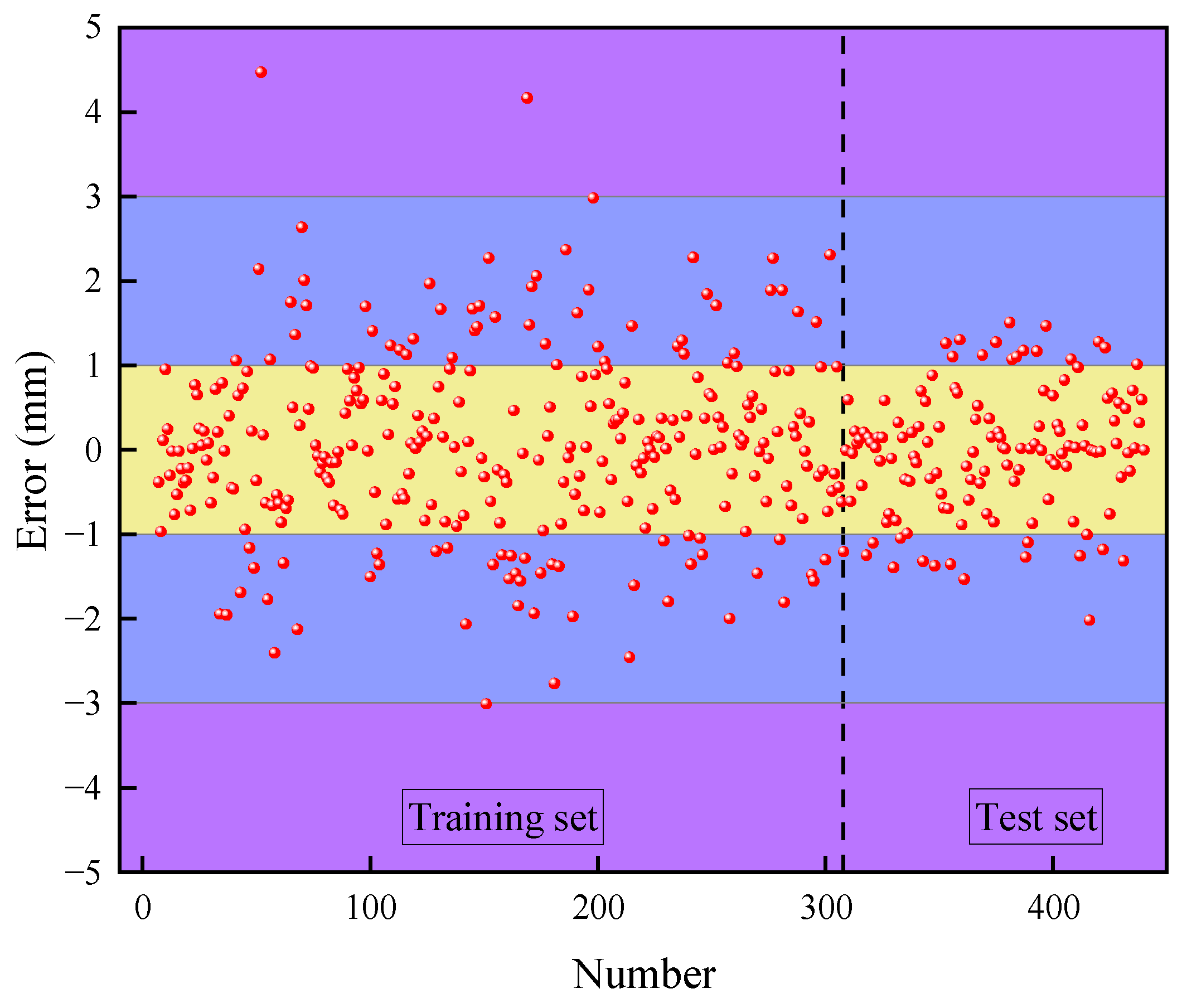
To further assess the discrepancy between the PSO-LSTM model’s predictions and the true values, the calculated prediction errors for slope surface displacements are presented in Figure 10.

As shown in Figure 10, a comparison of the sample error calculations from the PSO-LSTM model for predicting the slope surface displacement indicates that the maximum errors for the training set and the test set are 4.47 mm and −2.02 mm, respectively. Overall, approximately 70.7% of the samples exhibited prediction errors within ±1 mm, while about 99.3% of the samples demonstrated errors within ±3 mm. Notably, the maximum prediction error for the model’s test set is significantly smaller than that observed for the training set, suggesting that the PSO-LSTM model yields lower sample errors in predicting slope surface displacement. This finding further underscores the superior performance of the PSO-LSTM prediction model.

To extend the assessment of slope displacement, the previously constructed PSO-LSTM prediction model was employed to forecast displacement results for the subsequent 112 h, as illustrated in Figure 11.

To better visualize the stabilization trend of the data, we applied a fitting method to the predictions. Among the various fitting techniques available, the Gaussian fitting method is particularly effective in capturing the overall trend of the data. Given that the predicted dataset exhibits a single-peaked distribution, the Gaussian fitting method is suitable for modeling the prediction results.

As illustrated in Figure 11, analysis of the prediction results reveals that the slope surface displacements initially increase, followed by a decrease, and ultimately fluctuate around a stable value. Gaussian fitting indicates that the slope surface displacement eventually stabilizes, further validating the accuracy of the slope Level III warning results derived from multiple fractal eigenvalue analyses.

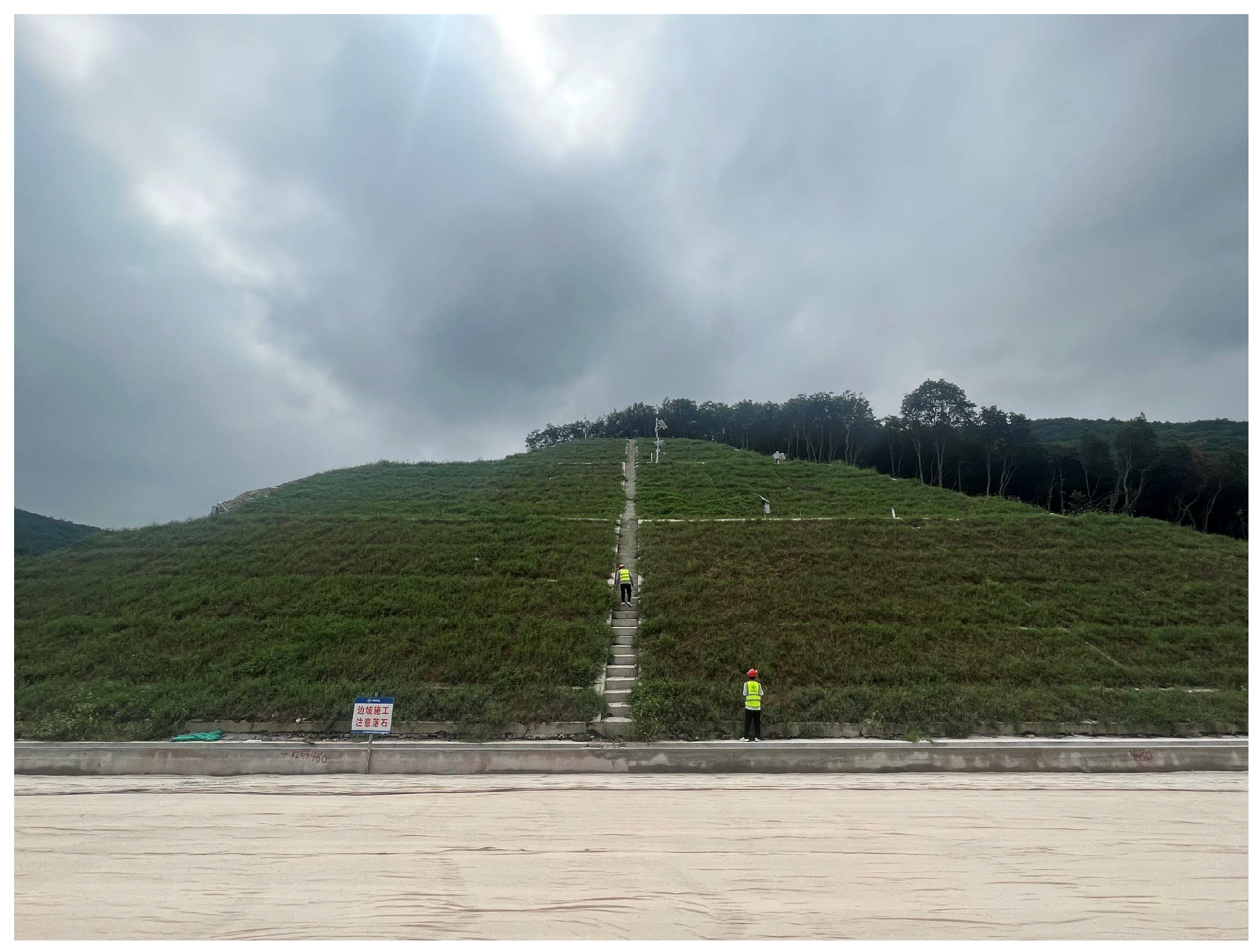
In summary, the results from the slope landslide warning levels and the predictions of slope surface displacements demonstrate a coherent response, indicating that the slope surface displacement is trending toward stability. Continuous monitoring and inspection are necessary to ensure the safety and stability of the slope. The slope site inspection is shown in Figure 12.

4. Conclusions

Analyzing and predicting the deformation patterns of slope surface displacements can provide essential technical support and theoretical guidance for early warning systems related to slope safety. This paper focuses on a slope in Zhuji, Zhejiang Province, combining on-site monitoring and measurement with multiple fractal analysis and a PSO-LSTM model to conduct an in-depth study of slope warning levels and surface displacement predictions. The main conclusions are as follows:

• The application of the MF-DFA method reveals that the slope surface displacements exhibit multiple fractal characteristics, indicating a stable developmental trend toward stabilization.
• The PSO-LSTM prediction model was employed to forecast the deformation trends of slope surface displacements. The results for the test set yielded R² = 0.91, MAE = 0.55, and RMSE = 0.72. The prediction errors associated with the PSO-LSTM model were minimal, demonstrating that the model effectively meets the requirements for slope surface displacement prediction.
• Synthesis of results from the analysis of multifractal characteristics and deformation predictions indicates that the current warning level for the slope is III, with subsequent deformations trending toward stabilization. Continued routine monitoring and inspections are recommended.
• The slopes analyzed in this study were characterized by a homogenous rock body and limited monitoring point locations. In future studies, a comprehensive fractal characterization of surface displacement monitoring results across multiple slopes with varying rock properties will be conducted. Additionally, numerical modeling of these slopes will be performed to further validate the accuracy of the proposed method. Additionally, incorporating more influencing factors related to slope deformation could further enhance the predictive accuracy of the PSO-LSTM model.

References

1. Cao, S.; Ye, H.; Zhan, Y. Cliff roads: An ecological conservation technique for road construction in mountainous regions of China. Landsc. Urban Plan 2010, 94, 228–233. [Google Scholar] [CrossRef]
2. Park, H.J.; West, T.R.; Woo, I. Probabilistic analysis of rock slope stability and random properties of discontinuity parameters, Interstate Highway 40, Western North Carolina, USA. Eng. Geol. 2005, 79, 230–250. [Google Scholar] [CrossRef]
3. Niu, P.; Zhou, A.; Huang, H. Assessing model of highway slope stability based on optimized SVM. China Geol. 2020, 3, 339–344. [Google Scholar] [CrossRef]
4. Lin, H.; Chang, S.; Wu, J.; Juang, C.H. Neural network-based model for assessing failure potential of highway slopes in the Alishan, Taiwan Area: Pre- and post-earthquake investigation. Eng. Geol. 2009, 104, 280–289. [Google Scholar] [CrossRef]
5. Shinoda, M.; Miyata, Y.; Kurokawa, U.; Kondo, K. Regional landslide susceptibility following the 2016 Kumamoto earthquake using back-calculated geomaterial strength parameters. Landslides 2019, 16, 1497–1516. [Google Scholar] [CrossRef]
6. Song, J.; Rodriguez-Marek, A.; Feng, T.; Ji, J. A generalized seismic sliding model of slopes with multiple slip surfaces. Earthq. Eng. Struct. D 2021, 50, 2595–2612. [Google Scholar] [CrossRef]
7. Chen, L.; Zhao, C.; Li, B.; He, K.; Ren, C.; Liu, X.; Liu, D. Deformation monitoring and failure mode research of mining-induced Jianshanying landslide in karst mountain area, China with ALOS/PALSAR-2 images. Landslides 2021, 18, 2739–2750. [Google Scholar] [CrossRef]
8. Kanungo, D.P.; Arora, M.K.; Sarkar, S.; Gupta, R.P. A comparative study of conventional, ANN black box, fuzzy and combined neural and fuzzy weighting procedures for landslide susceptibility zonation in Darjeeling Himalayas. Eng. Geol. 2006, 85, 347–366. [Google Scholar] [CrossRef]
9. Kundu, S.; Saha, A.K.; Sharma, D.C.; Pant, C.C. Remote Sensing and GIS Based Landslide Susceptibility Assessment using Binary Logistic Regression Model: A Case Study in the Ganeshganga Watershed, Himalayas. J. Indian Soc. Remote 2013, 41, 697–709. [Google Scholar] [CrossRef]
10. Wubalem, A.; Meten, M. Landslide susceptibility mapping using information value and logistic regression models in Goncha Siso Eneses area, northwestern Ethiopia. SN Appl. Sci. 2020, 2, 807. [Google Scholar] [CrossRef]
11. Ayalew, L.; Yamagishi, H. Slope failures in the Blue Nile basin, as seen from landscape evolution perspective. Geomorphology 2004, 57, 95–116. [Google Scholar] [CrossRef]
12. Temesgen, B.; Mohammed, M.U.; Korme, T. Natural hazard assessment using GIS and remote sensing methods, with particular reference to the landslides in the Wondogenet area, Ethiopia. Phys. Chem. Earth Part C—Sol. Terrestial Planet. Sci. 2001, 26, 665–675. [Google Scholar] [CrossRef]
13. Singh, T.N.; Gulati, A.; Dontha, L.; Bhardwaj, V. Evaluating cut slope failure by numerical analysis—A case study. Nat. Hazards 2008, 47, 263–279. [Google Scholar] [CrossRef]
14. Ramakrishnan, D.; Singh, T.N.; Verma, A.K.; Gulati, A.; Tiwari, K.C. Soft computing and GIS for landslide susceptibility assessment in Tawaghat area, Kumaon Himalaya, India. Nat. Hazards 2013, 65, 315–330. [Google Scholar] [CrossRef]
15. Cheng, Y.M.; Lansivaara, T.; Wei, W.B. Two-dimensional slope stability analysis by limit equilibrium and strength reduction methods: Reply. Comput. Geotech. 2008, 35, 309–311. [Google Scholar] [CrossRef]
16. Liu, S.Y.; Shao, L.T.; Li, H.J. Slope stability analysis using the limit equilibrium method and two finite element methods. Comput. Geotech. 2015, 63, 291–298. [Google Scholar] [CrossRef]
17. Morales-Esteban, A.; Luis De Justo, J.; Reyes, J.; Miguel Azanon, J.; Durand, P.; Martinez-Alvarez, F. Stability analysis of a slope subject to real accelerograms by finite elements. Application to San Pedro cliff at the Alhambra in Granada. Soil Dyn. Earthq. Eng. 2015, 69, 28–45. [Google Scholar] [CrossRef]
18. Stianson, J.R.; Chan, D.; Fredlund, D.G. Role of admissibility criteria in limit equilibrium slope stability methods based on finite element stresses. Comput. Geotech. 2015, 66, 113–125. [Google Scholar] [CrossRef]
19. Moawwez, M.A.; Wang, J.; Hussain, M.A. Development of empirical correlations for limit equilibrium methods of slope stability analysis. Arab. J. Geosci. 2021, 14, 2020. [Google Scholar] [CrossRef]
20. Tesfaye, M.; Regassa, B.; Garo, T. Rock slope stability modeling using kinematic and limit equilibrium methods along Woliso to Wonchi lake road, central Ethiopia. Model. Earth Syst. Environ. 2024, 10, 331–347. [Google Scholar] [CrossRef]
21. Deparis, J.; Garambois, S.; Hantz, D. On the potential of Ground Penetrating Radar to help rock fall hazard assessment: A case study of a limestone slab, Gorges de la Bourne (French Alps). Eng. Geol. 2007, 94, 89–102. [Google Scholar] [CrossRef]
22. Medeiros Santos, A.E.; Lana, M.S.; Cabral, I.E.; Pereira, T.M.; Naghadehi, M.Z.; Santos Da Silva, D.D.F.; Dos Santos, T.B. Evaluation of Rock Slope Stability Conditions Through Discriminant Analysis. Geotech. Geol. Eng. 2019, 37, 775–802. [Google Scholar] [CrossRef]
23. Sarkar, S.; Kanungo, D.P.; Kumar, S. Rock Mass Classification and Slope Stability Assessment of Road Cut Slopes in Garhwal Himalaya, India. Geotech. Geol. Eng. 2012, 30, 827–840. [Google Scholar] [CrossRef]
24. Vishal, V.; Siddique, T.; Purohit, R.; Phophliya, M.K.; Pradhan, S.P. Hazard assessment in rockfall-prone Himalayan slopes along National Highway-58, India: Rating and simulation. Nat. Hazards 2017, 85, 487–503. [Google Scholar] [CrossRef]
25. Verma, A.K.; Kumar, N.; Sardana, S.; Singh, T.N. Rockfall Analysis and Optimized Design of Rockfall Barrier Along a Strategic Road near Solang Valley, Himachal Pradesh, India. Indian Geotech. J. 2018, 48, 686–699. [Google Scholar] [CrossRef]
26. Sardana, S.; Verma, A.K.; Verma, R.; Singh, T.N. Rock slope stability along road cut of Kulikawn to Saikhamakawn of Aizawl, Mizoram, India. Nat. Hazards 2019, 99, 753–767. [Google Scholar] [CrossRef]
27. Sardana, S.; Verma, A.K.; Singh, A.; Laldinpuia. Comparative analysis of rockmass characterization techniques for the stability prediction of road cut slopes along NH-44A, Mizoram, India. Bull. Eng. Geol. Environ. 2019, 78, 5977–5989. [Google Scholar] [CrossRef]
28. Cignetti, M.; Godone, D.; Wrzesniak, A.; Giordan, D. Structure from Motion Multisource Application for Landslide Characterization and Monitoring: The Champlas du Col Case Study, Sestriere, North-Western Italy. Sensors 2019, 19, 2364. [Google Scholar] [CrossRef]
29. Do, T.M.T.; Artieres, T. Learning mixture models with support vector machines for sequence classification and segmentation. Pattern Recogn. 2009, 42, 3224–3230. [Google Scholar] [CrossRef]
30. Yang, Y.; Song, S.; Yue, F.; He, W.; Shao, W.; Zhao, K.; Nie, W. Superpixel-based automatic image recognition for landslide deformation areas. Eng. Geol. 2019, 259, 105166. [Google Scholar] [CrossRef]
31. Li, Q.; Song, D.; Yuan, C.; Nie, W. An image recognition method for the deformation area of open-pit rock slopes under variable rainfall. Measurement 2022, 188, 110544. [Google Scholar] [CrossRef]
32. Wang, G.; Zhao, B.; Wu, B.; Zhang, C.; Liu, W. Intelligent prediction of slope stability based on visual exploratory data analysis of 77 in situ cases. Int. J. Min. Sci. Technol. 2023, 33, 47–59. [Google Scholar] [CrossRef]
33. Lin, S.; Zheng, H.; Han, B.; Li, Y.; Han, C.; Li, W. Comparative performance of eight ensemble learning approaches for the development of models of slope stability prediction. Acta Geotech. 2022, 17, 1477–1502. [Google Scholar] [CrossRef]
34. Zhang, W.; Li, H.; Han, L.; Chen, L.; Wang, L. Slope stability prediction using ensemble learning techniques: A case study in Yunyang County, Chongqing, China. J. Rock Mech. Geotech. 2022, 14, 1089–1099. [Google Scholar] [CrossRef]
35. Qi, C.; Tang, X. Slope stability prediction using integrated metaheuristic and machine learning approaches: A comparative study. Comput. Ind. Eng. 2018, 118, 112–122. [Google Scholar] [CrossRef]
36. Kardani, N.; Zhou, A.; Nazem, M.; Shen, S. Improved prediction of slope stability using a hybrid stacking ensemble method based on finite element analysis and field data. J. Rock Mech. Geotech. 2021, 13, 188–201. [Google Scholar] [CrossRef]
37. Khanh, P.; Kim, D.; Park, S.; Choi, H. Ensemble learning-based classification models for slope stability analysis. Catena 2021, 196, 104886. [Google Scholar] [CrossRef]
38. Dong, Y.; Lan, Y.; Li, B.; Li, W. Study on deformation characteristics and early warning analysis of rainfall-type shallow soil landslides—Tongnan Orchard in Chongqing as an example. Yangtze River 2020, 51, 97–101. [Google Scholar] [CrossRef]
39. Deng, X. Landslide deformation stability evaluation and early warning analysis based on information decomposition. Yangtze River 2021, 52, 101–107. [Google Scholar] [CrossRef]
40. Zhou, Z.; Shen, J.; Shu, J.; Duan, W.; Yang, R.; Li, Y. Study of prediction and early warning of slope deformation of accumulation layer in front of a hydropower station dam in Southwest China. J. Chengdu Univ. Technol. (Sci. Technol. Ed.) 2020, 47, 481–491. [Google Scholar]
41. Lei, H.; Zhou, X.; Wang, Y. Research on landslide early warning and prediction based on combined response of multifractal characteristics and sub item prediction. J. Geod. Geodyn. 2022, 42, 885–891. [Google Scholar] [CrossRef]
42. Mao, H.; Zhang, M.; Li, B.; Xu, N. Stability Analysis of the Left Bank Slope of Baihetan Hydropower Station Based on the MF-DFA Method. Adv. Civ. Eng. 2020, 2020, 8898318. [Google Scholar] [CrossRef]
43. Ding, L.; Li, C.; Lei, Z.; Zhang, C.; Wei, L.; Guo, Z.; Li, Y.; Fan, X.; Qi, D.; Wang, J. Spatiotemporal evolution of deformation and LSTM prediction model over the slope of the deep excavation section at the head of the South-North Water Transfer Middle Route Canal. Heliyon 2024, 10, e26301. [Google Scholar] [CrossRef]
44. Xu, J.; Hou, X.; Wu, X.; Liu, Y.; Sun, G. Research on slope displacement prediction based on MIC-XGBoost-LSTM model. China J. Highw. Transp. 2024, 1–12. Available online: https://kns.cnki.net/KCMS/detail/detail.aspx?dbcode=CAPJ&dbname=CAPJLAST&filename=ZGGL20240221002&uniplatform=OVERSEA&v=1DM6sN0rIQ2AlZhs-Qi66TChuhveI3aSVq8otiIQOGTZAw56q-C9LbQiyTY2598- (accessed on 26 February 2024).
45. Xiao, H.; Wang, S.; Chen, L.; Fan, Y.; Wan, J. An optimization network model for slope deformation prediction based on GA and LSTM fusion and tis application. J. Geod. Geodyn. 2024, 44, 491–496. [Google Scholar] [CrossRef]
46. Yang, S.; Jin, A.; Nie, W.; Liu, C.; Li, Y. Research on SSA-LSTM-Based Slope Monitoring and Early Warning Model. Sustainability 2022, 14, 10246. [Google Scholar] [CrossRef]
47. Yang, X.; Fan, X.; Wang, K.; Zhou, Z. Research on landslide susceptibility prediction model based on LSTM-RF-MDBN. Environ. Sci. Pollut. R 2024, 31, 1543–1561. [Google Scholar] [CrossRef]
48. Zhang, X.; Zhu, C.; He, M.; Dong, M.; Zhang, G.; Zhang, F. Failure Mechanism and Long Short-Term Memory Neural Network Model for Landslide Risk Prediction. Remote Sens. 2022, 14, 166. [Google Scholar] [CrossRef]
49. Lin, Z.; Sun, X.; Ji, Y. Landslide Displacement Prediction Model Using Time Series Analysis Method and Modified LSTM Model. Electronics 2022, 11, 1519. [Google Scholar] [CrossRef]
50. Khalili, M.A.; Guerriero, L.; Pouralizadeh, M.; Calcaterra, D.; Di Martire, D. Monitoring and prediction of landslide-related deformation based on the GCN-LSTM algorithm and SAR imagery. Nat. Hazards 2023, 119, 39–68. [Google Scholar] [CrossRef]
51. Xiong, Y. Correlation analysis between multifractal characteristics of regional geomorphology and development of geological disasters. Earth Sci. Res. J. 2021, 25, 49–55. [Google Scholar] [CrossRef]
52. Sun, B.; Ren, F.; Liu, D. Research on the failure precursors of layered slate based on multifractal characteristics of acoustic emission. Rock Soil Mech. 2022, 43, 749–760. [Google Scholar] [CrossRef]
53. Yang, C.; Huang, R.; Liu, D.; Qiu, W.; Zhang, R.; Tang, Y. Analysis and Warning Prediction of Tunnel Deformation Based on Multifractal Theory. Fractal Fract. 2024, 8, 108. [Google Scholar] [CrossRef]
54. Niu, Y.; Liu, P.; Zhang, C.; Hu, Y.; Wang, J. Mechanical properties and dynamic multifractal characteristics of shale under anisotropic stress using AE technology. Geoenergy Sci. Eng. 2023, 226, 211748. [Google Scholar] [CrossRef]
55. Telesca, L.; Chamoli, A.; Lovallo, M.; Stabile, T.A. Investigating the Tsunamigenic Potential of Earthquakes from Analysis of the Informational and Multifractal Properties of Seismograms. Pure Appl. Geophys. 2015, 172, 1933–1943. [Google Scholar] [CrossRef]
Figure 1. Site plan of the slope: (a) slopes, (b) monitoring devices.
Fractalfract 08 00522 g001
Figure 2. Displacement–time diagram of the surface layer of the slope.
Fractalfract 08 00522 g002
Figure 3. Flowchart of MF-DFA calculation.
Fractalfract 08 00522 g003
Figure 4. Flowchart of PSO algorithm.
Fractalfract 08 00522 g004
Figure 5. q -order fluctuation function l o g F q s l o g s trend plot of double logarithmic fit: (a) Group I, (b) Group II, (c) Group III, (d) Group IV.
Fractalfract 08 00522 g005aFractalfract 08 00522 g005b
Figure 6. Variation of each index of displacement series: (a) generalized Hurst index, (b) scale function τ , q .
Fractalfract 08 00522 g006
Figure 7. Multiple fractal spectra of surface displacements for each group of side slopes.
Fractalfract 08 00522 g007
Figure 8. Values of slope landslide warning parameters: (a) Δ α parameter values, (b) Δ f ( α ) parameter values.
Fractalfract 08 00522 g008
Figure 9. Predicted results of slope surface displacements.
Fractalfract 08 00522 g009
Figure 10. Error map of slope displacement prediction.
Fractalfract 08 00522 g010
Figure 11. Predicted and fitted slope displacements.
Fractalfract 08 00522 g011
Figure 12. Slope site walk-through map.
Fractalfract 08 00522 g012