Analysis of Truncated M-Fractional Mathematical and Physical (2+1)-Dimensional Nonlinear Kadomtsev–Petviashvili-Modified Equal-Width Model

Abstract

This study focuses on the mathematical and physical analysis of a truncated M-fractional (2+1)-dimensional nonlinear Kadomtsev–Petviashvili-modified equal-width model. The distinct types of the exact wave solitons of an important real-world equation called the truncated M-fractional (2+1)-dimensional nonlinear Kadomtsev–Petviashvili-modified equal-width (KP-mEW) model are achieved. This model is used to explain ocean waves, matter-wave pulses, waves in ferromagnetic media, and long-wavelength water waves. The diverse patterns of waves on the oceans are yielded by the Kadomtsev–Petviashvili-modified equal-width (KP-mEW) equation. We obtain kink-, bright-, and periodic-type soliton solutions by using the ${exp}_a$ function and modified extended tanh function methods. The solutions are more valuable than the existing results due to the use of a truncated M-fractional derivative. These solutions may be useful in different areas of science and engineering. The methods applied are simple and useful.

1. Introduction

Mathematical modeling has much importance in applied sciences and engineering. Many models in the fields of applied sciences and engineering have been developed, such as the new generalized Bogoyavlensky–Konopelchenko model [1], Sharma–Tasso–Olver– Burgers model [2], Oskolkov model [3], generalized Kadomtsev–Petviashvili model [4], Biswas–Arshed model [5], Kundu–Mukherjee–Naskar model [6], extended Fisher–Kolmogorov model [7], generalized regularized long-wave model [8], nonlinear integrable wave equations [9], bi-Hamiltonian system [10], new extended Sakovich equations [11], nano-ionic current model [12], modified Schrödinger’s equation [13], perturbed nonlinear Schrödinger equation [14], and many more.

In this paper, we used two simple and useful methods: the ${exp}_a$ function method and the modified extended tanh function method. These methods have various applications. For example, the optical soliton solutions of zig-zag optical lattices are obtained by applying the ${exp}_a$ function method [15], the optical solitons of the Sasa–Satsuma model are gained by using the ${exp}_a$ function scheme [16], and different optical solitons of the perturbed Gerdjikov–Ivanov model are obtained with the use of the ${exp}_a$ function method [17]. Distinct kinds of analytical wave solutions of the Lakshmanan–Porsezian–Daniel model were obtained by applying the modified extended tanh function scheme [18], and some traveling wave solutions of the coupled Klein–Gordon–Zakharov equation were attained in [19].

The (2+1)-dimensional nonlinear Kadomtsev–Petviashvili-modified equal-width (KP-mEW) equation is one of the mathematical fluid models used in dynamics, engineering, etc. Different kinds of exact wave solutions are achieved in the literature by using different methods. For instance, some of the soliton solutions are obtained by using the rational $(G^{\prime }/G)$-expansion technique and improved tanh function method in [20], and the bell, anti-bell, singular kink, anti-kink, and other kinds of solitons are gained by the improved auxiliary equation technique and enhanced rational $(G^{\prime }/G)$-expansion technique in [21].

The purpose of this paper is to find new kinds of truncated M-fractional exact soliton solutions for the (2+1)-dimensional nonlinear Kadomtsev–Petviashvili-modified equal-width (KP-mEW) equation by employing the ${exp}_a$ function and modified extended tanh function methods.

The motivation of this paper is to determine the new types of exact soliton solutions of the KP-mEW equation with a truncated M-fractional derivative. The effect of this derivative is also explained. The truncated M-fractional derivative fulfills the characteristics of both integer and fractional derivatives. The truncated M-fractional derivative provides closer solutions to the numerical solutions. This definition of derivatives provides more valuable results than the other definitions of derivatives. The truncated M-fractional derivative is used for the first time in our model. The gained solutions include dark, bright, singular, kink, dark singular, dark solitary and other solutions. The obtained solutions are useful in many areas of mathematical physics. The used methods explore different types of solutions. Both methods are not used for the model concerned in the literature. These methods are easy to use for solving nonlinear fractional partial differential equations (NLFPDEs). These methods are applicable for all NLFPDEs.

There are distinct sections in this paper: Section 2 gives the description of the methods; Section 3 introduces the model description and mathematical analysis; Section 4 shows the exact wave solutions of the concerned model; Section 5 is about the physical interpretation; and Section 6 presents the conclusion.

2. Description of Strategies

2.1. $ex{p}_a$ Function Method

Assuming the nonlinear PDE,

$$S(g,g^2{g}_x,g_t,g_{xx},g_{tt},g_{xt},...)=0.$$

(1)

Equation (1) yields:

$$T(G,G^2{G}^{\prime },G^{\prime },G^{\prime \prime },...,)=0.$$

(2)

by using the transformation:

$$g(x,t)=G\left(\xi \right),\xi =\delta x+\lambda t.$$

(3)

Here, $\delta$ and $\lambda$ represent the amplitude and speed of the wave, while x and t are the spatial and temporal independent variables, respectively. Considering that the solutions of Equation (3) are [22,23,24,25]:

$$G\left(\xi \right)={\displaystyle \frac{{\alpha }_0+{\alpha }_1{d}^{\xi }+...+{\alpha }_m{d}^{m\xi }}{{\beta }_0+{\beta }_1{d}^{\xi }+...+{\beta }_m{d}^{m\xi }}},d\ne 0,1.$$

(4)

here, d is a free parameter and it can take positive values except for 1, where ${\alpha }_i$ and ${\beta }_i(0\le i\le m)$ are unknowns. The value of m is calculated by the Homogeneous Balance method in Equation (2). Using Equation (4) in Equation (2) provides

$$\wp \left(d^{\xi }\right)={\ell }_0+{\ell }_1{d}^{\xi }+...+{\ell }_n{d}^{n\xi }=0.$$

(5)

By putting ${\ell }_i(0\le i\le n)$ into Equation (5) and considering it to be equal to zero, a system of equations is achieved:

$${\ell }_i=0,herei=0,...,n.$$

(6)

By applying the gained distinct solution sets, the exact solutions for Equation (1) are obtained.

2.2. Modified Extended Tanh Function Method

Here, some of the main steps of the method are given. Assuming a conformable fractional NLPDE:

$$S(g,g^2{g}_x,g_t,g_{xx},g_{tt},g_{xt},...)=0.$$

(7)

where $g=g(x,t)$ shows a wave function. Considering the following wave transformation:

$$g(x,t)=G\left(\xi \right),\xi =\mu (x+-\nu t).$$

(8)

here, $\nu$ denotes the soliton velocity while $\mu$ is a constant with effects on both the spatial and temporal variables. Putting Equation (8) into Equation (7) yields:

$$\chi (G,\mu G^2{G}^{\prime },\mu G^{\prime },\mu {\nu }^2{G}^{\prime \prime },...)=0.$$

(9)

Considering the solution of Equation (9), shown as:

$$G\left(\xi \right)=a_0+\sum _{i=1}^m{a}_i{\phi }^i\left(\xi \right)+\sum _{i=1}^m{b}_i{\phi }^{-i}\left(\xi \right).$$

(10)

Here, $a_0,a_i,b_i,(i=1,2,3,...,m)$ are undetermined.

Here $\phi \left(\xi \right)$ fulfills the following:

$${\phi }^{\prime }\left(\xi \right)=\rho +{\phi }^2\left(\xi \right).$$

(11)

Here, $\rho$ is a constant and the solution of Equation (11) is shown in [26]:

• Case 1: if $\rho <0$:

$$\phi \left(\xi \right)=-\sqrt{-\rho }tanh\left(\sqrt{-\rho }\xi \right),$$

(12)

or

$$\phi \left(\xi \right)=-\sqrt{-\rho }coth\left(\sqrt{-\rho }\xi \right).$$

(13)

Case 2: if $\rho =0$:

$$\phi \left(\xi \right)={\displaystyle \frac{-1}{\xi }}.$$

(14)

Case 3: if $\rho >0$:

$$\phi \left(\xi \right)=\sqrt{\rho }tan\left(\sqrt{\rho }\xi \right),$$

(15)

or

$$\phi \left(\xi \right)=-\sqrt{\rho }cot\left(\sqrt{\rho }\xi \right).$$

(16)

By putting Equation (10) into Equation (9) along with Equation (11) and summing up the coefficient of $\phi \left(\xi \right)$ of every power and setting it to 0, we achieve sets of algebraic equations containing $a_0,a_i,b_i(i=1,2,3...,m)$ and $\rho$. Solving the system yields the different solution sets for Equation (7).

3. Model Description and Mathematical Analysis

Our model, which is called the Kadomtsev–Petviashvili-modified equal-width equation, is a physically appearing model. This model is observed in ocean waves, water waves, and other kinds of waves.

The truncated M-fractional (2+1)-dimensional nonlinear Kadomtsev–Petviashvili-modified equal-width (KP-mEW) equation is given as:

$$D_{M,x}^{\alpha ,\mathrm{{\rm Y}}}(D_{M,t}^{\alpha ,\mathrm{{\rm Y}}}u+\delta D_{M,t}^{\alpha ,\mathrm{{\rm Y}}}\left(u^3\right)-\tau D_{M,xxt}^{3\alpha ,\mathrm{{\rm Y}}}u)+D_{M,2y}^{2\alpha ,\mathrm{{\rm Y}}}u=0.$$

(17)

where

$$D_{M,x}^{\alpha ,\mathrm{{\rm Y}}}u=\underset{\tau \to 0}{lim}{\displaystyle \frac{v\left(x{E}_{\mathrm{Y}}\left(\tau x^{1-\alpha }\right)\right)-u\left(x\right)}{\tau }},\alpha \in (0,1],\mathrm{Y}\in (0,\infty ),$$

(18)

Here, $E_{\mathrm{Y}}(.)$ shows a Mittag-Leffler function [27,28].

In Equation (17), $u=u(x,y,t)$ denotes the wave function. This model was discovered by Wazwaz [29] and is a combined form of the Kadomtsev–Petviashvili (KP) equation and the modified equal-width (mEW) equation. Equation (17) is used to explain ocean waves, matter-wave pulses, waves in ferromagnetic media, and long-wavelength water waves along frequency dispersions and faintly nonlinear reinstating forces.

Assuming the transformations are shown as

$$u=U\left(\xi \right);\xi ={\displaystyle \frac{1}{\alpha }}\mathrm{\Gamma }(\mathrm{Y}+1)(x^{\alpha }+y^{\alpha }-\lambda t^{\alpha }),$$

(19)

here, $\lambda$ indicates the soliton speed. Substituting Equation (19) into Equation (17) results in

$$\delta U^3-\lambda \tau U^{\prime \prime }+U(\theta -\lambda )=0.$$

(20)

We obtain the value of m by utilizing the Homogeneous Balance scheme in Equation (20) as follows:

By balancing the terms $U^3$ and $U^{"}$, we obtain

$3m=m+2$, so $m=1$.

In the next section, the exact wave solitons of Equation (20) will be found by using two methods.

4. Exact Wave Solutions

4.1. By $ex{p}_a$ Function Method

Equation (4) transforms into the given form for $m=1$:

$$U\left(\xi \right)={\displaystyle \frac{{\alpha }_0+{\alpha }_1{d}^{\xi }}{{\beta }_0+{\beta }_1{d}^{\xi }}},$$

(21)

where ${\alpha }_0$, ${\alpha }_1$, ${\beta }_0$, and ${\beta }_1$ are unknowns. A set of equations is acquired by entering Equation (21) into Equation (20) and setting the coefficients of each power of $d^{\xi }$ and constant term to 0. By using Mathematica to solve the obtained system, we discover the following solution sets:

• Set 1:

$$\left\{{\alpha }_0={\displaystyle \frac{{\beta }_0\sqrt{\theta }\sqrt{\tau }log\left(d\right)}{\sqrt{-\delta \left(\tau {log}^2\left(d\right)-2\right)}}},{\alpha }_1=-\sqrt{{\displaystyle \frac{{\beta }_1^2\theta \tau {log}^2\left(d\right)}{2\delta -\delta \tau {log}^2\left(d\right)}}},\lambda =-{\displaystyle \frac{2\theta }{\tau {log}^2\left(d\right)-2}}\right\}.$$

(22)

$$u(x,y,t)={\displaystyle \frac{\sqrt{\theta }\sqrt{\tau }log\left(d\right)}{\sqrt{-\delta \left(\tau {log}^2\left(d\right)-2\right)}}}({\displaystyle \frac{{\beta }_0-{\beta }_1{d}^{\frac{\mathrm{\Gamma }(1+\mathrm{{\rm Y}})}{\alpha }(x^{\alpha }+y^{\alpha }-\lambda t^{\alpha })}}{{\beta }_0+{\beta }_1{d}^{\frac{\mathrm{\Gamma }(1+\mathrm{{\rm Y}})}{\alpha }(x^{\alpha }+y^{\alpha }-\lambda t^{\alpha })}}}).$$

(23)

Set 2:

$$\left\{{\alpha }_0=-{\displaystyle \frac{{\beta }_0\sqrt{\theta }\sqrt{\tau }log\left(d\right)}{\sqrt{-\delta \left(\tau {log}^2\left(d\right)-2\right)}}},{\alpha }_1=\sqrt{{\displaystyle \frac{{\beta }_1^2\theta \tau {log}^2\left(d\right)}{2\delta -\delta \tau {log}^2\left(d\right)}}},\lambda =-{\displaystyle \frac{2\theta }{\tau {log}^2\left(d\right)-2}}\right\}.$$

(24)

$$u(x,y,t)=-{\displaystyle \frac{\sqrt{\theta }\sqrt{\tau }log\left(d\right)}{\sqrt{-\delta \left(\tau {log}^2\left(d\right)-2\right)}}}({\displaystyle \frac{{\beta }_0-{\beta }_1{d}^{\frac{\mathrm{\Gamma }(1+\mathrm{{\rm Y}})}{\alpha }(x^{\alpha }+y^{\alpha }-\lambda t^{\alpha })}}{{\beta }_0+{\beta }_1{d}^{\frac{\mathrm{\Gamma }(1+\mathrm{{\rm Y}})}{\alpha }(x^{\alpha }+y^{\alpha }-\lambda t^{\alpha })}}}).$$

(25)

where ${\beta }_0$ and ${\beta }_1$ are the free parameters.

4.2. Application to the Modified Extended $tanh$ Function Method

For $m=1$, Equation (10) is reduced to:

$$U\left(\xi \right)=a_0+a_1\phi \left(\xi \right)+b_1\phi {\left(\xi \right)}^{-1},$$

(26)

where $a_0$, $a_1$, and $b_1$ are the unknowns. Using Equation (26) in Equation (20) along with Equation (11) and by collecting the coefficients of each power of $\phi \left(\xi \right)$, we obtain a system containing $a_0$, $a_1$, $b_1$, $\lambda$, and $\rho$. Solving the system yields the following solution sets:

• Set 1:

$$\left\{{\alpha }_0=0,{\alpha }_1=-{\displaystyle \frac{\sqrt{2}\sqrt{\theta }\sqrt{\tau }}{\sqrt{\delta -4\delta \rho \tau }}},{\beta }_1=-{\displaystyle \frac{\sqrt{2}\sqrt{\theta }\rho \sqrt{\tau }}{\sqrt{\delta -4\delta \rho \tau }}},\lambda ={\displaystyle \frac{\theta }{1-4\rho \tau }}\right\}.$$

(27)

Case 1: For $\rho <0$:

$$\begin{array}{c}u(x,y,t)=-{\displaystyle \frac{\sqrt{2}\sqrt{\theta }\sqrt{\tau }}{\sqrt{\delta -4\delta \rho \tau }}}(-\sqrt{-\rho }tanh(\sqrt{-\rho }{\displaystyle \frac{\mathrm{\Gamma }(1+\mathrm{{\rm Y}})}{\alpha }}(x^{\alpha }+y^{\alpha }-{\displaystyle \frac{\theta }{1-4\rho \tau }}{t}^{\alpha }))+\hfill \\ \hfill {\displaystyle \frac{\rho }{-\sqrt{-\rho }tanh(\sqrt{-\rho }\frac{\mathrm{\Gamma }(1+\mathrm{{\rm Y}})}{\alpha }(x^{\alpha }+y^{\alpha }-\frac{\theta }{1-4\rho \tau }{t}^{\alpha }))}}),\end{array}$$

(28)

or

$$\begin{array}{c}u(x,y,t)=-{\displaystyle \frac{\sqrt{2}\sqrt{\theta }\sqrt{\tau }}{\sqrt{\delta -4\delta \rho \tau }}}(-\sqrt{-\rho }coth(\sqrt{-\rho }{\displaystyle \frac{\mathrm{\Gamma }(1+\mathrm{{\rm Y}})}{\alpha }}(x^{\alpha }+y^{\alpha }-{\displaystyle \frac{\theta }{1-4\rho \tau }}{t}^{\alpha }))+\hfill \\ \hfill {\displaystyle \frac{\rho }{-\sqrt{-\rho }coth(\sqrt{-\rho }\frac{\mathrm{\Gamma }(1+\mathrm{{\rm Y}})}{\alpha }(x^{\alpha }+y^{\alpha }-\frac{\theta }{1-4\rho \tau }{t}^{\alpha }))}}).\end{array}$$

(29)

Case 3: For $\rho >0$:

$$\begin{array}{c}u(x,y,t)=-{\displaystyle \frac{\sqrt{2}\sqrt{\theta }\sqrt{\tau }}{\sqrt{\delta -4\delta \rho \tau }}}(\sqrt{\rho }tan(\sqrt{\rho }{\displaystyle \frac{\mathrm{\Gamma }(1+\mathrm{{\rm Y}})}{\alpha }}(x^{\alpha }+y^{\alpha }-{\displaystyle \frac{\theta }{1-4\rho \tau }}{t}^{\alpha }))+\hfill \\ \hfill {\displaystyle \frac{\rho }{\sqrt{\rho }tan(\sqrt{\rho }\frac{\mathrm{\Gamma }(1+\mathrm{{\rm Y}})}{\alpha }(x^{\alpha }+y^{\alpha }-\frac{\theta }{1-4\rho \tau }{t}^{\alpha }))}}),\end{array}$$

(30)

or

$$\begin{array}{c}u(x,y,t)=-{\displaystyle \frac{\sqrt{2}\sqrt{\theta }\sqrt{\tau }}{\sqrt{\delta -4\delta \rho \tau }}}(-\sqrt{\rho }cot(\sqrt{\rho }{\displaystyle \frac{\mathrm{\Gamma }(1+\mathrm{{\rm Y}})}{\alpha }}(x^{\alpha }+y^{\alpha }-{\displaystyle \frac{\theta }{1-4\rho \tau }}{t}^{\alpha }))+\hfill \\ \hfill {\displaystyle \frac{\rho }{-\sqrt{\rho }cot(\sqrt{\rho }\frac{\mathrm{\Gamma }(1+\mathrm{{\rm Y}})}{\alpha }(x^{\alpha }+y^{\alpha }-\frac{\theta }{1-4\rho \tau }{t}^{\alpha }))}}).\end{array}$$

(31)

Set 2:

$$\left\{{\alpha }_0=0,{\alpha }_1={\displaystyle \frac{\sqrt{2}\sqrt{\theta }\sqrt{\tau }}{\sqrt{\delta -4\delta \rho \tau }}},{\beta }_1={\displaystyle \frac{\sqrt{2}\sqrt{\theta }\rho \sqrt{\tau }}{\sqrt{\delta -4\delta \rho \tau }}},\lambda ={\displaystyle \frac{\theta }{1-4\rho \tau }}\right\}.$$

(32)

Case 1: For $\rho <0$:

$$\begin{array}{c}u(x,y,t)={\displaystyle \frac{\sqrt{2}\sqrt{\theta }\sqrt{\tau }}{\sqrt{\delta -4\delta \rho \tau }}}(-\sqrt{-\rho }tanh(\sqrt{-\rho }{\displaystyle \frac{\mathrm{\Gamma }(1+\mathrm{{\rm Y}})}{\alpha }}(x^{\alpha }+y^{\alpha }-{\displaystyle \frac{\theta }{1-4\rho \tau }}{t}^{\alpha }))+\hfill \\ \hfill {\displaystyle \frac{\rho }{-\sqrt{-\rho }tanh(\sqrt{-\rho }\frac{\mathrm{\Gamma }(1+\mathrm{{\rm Y}})}{\alpha }(x^{\alpha }+y^{\alpha }-\frac{\theta }{1-4\rho \tau }{t}^{\alpha }))}}),\end{array}$$

(33)

or

$$\begin{array}{c}u(x,y,t)={\displaystyle \frac{\sqrt{2}\sqrt{\theta }\sqrt{\tau }}{\sqrt{\delta -4\delta \rho \tau }}}(-\sqrt{-\rho }coth(\sqrt{-\rho }{\displaystyle \frac{\mathrm{\Gamma }(1+\mathrm{{\rm Y}})}{\alpha }}(x^{\alpha }+y^{\alpha }-{\displaystyle \frac{\theta }{1-4\rho \tau }}{t}^{\alpha }))+\hfill \\ \hfill {\displaystyle \frac{\rho }{-\sqrt{-\rho }coth(\sqrt{-\rho }\frac{\mathrm{\Gamma }(1+\mathrm{{\rm Y}})}{\alpha }(x^{\alpha }+y^{\alpha }-\frac{\theta }{1-4\rho \tau }{t}^{\alpha }))}}).\end{array}$$

(34)

Case 3: For $\rho >0$:

$$\begin{array}{c}u(x,y,t)={\displaystyle \frac{\sqrt{2}\sqrt{\theta }\sqrt{\tau }}{\sqrt{\delta -4\delta \rho \tau }}}(\sqrt{\rho }tan(\sqrt{\rho }{\displaystyle \frac{\mathrm{\Gamma }(1+\mathrm{{\rm Y}})}{\alpha }}(x^{\alpha }+y^{\alpha }-{\displaystyle \frac{\theta }{1-4\rho \tau }}{t}^{\alpha }))+\hfill \\ \hfill {\displaystyle \frac{\rho }{\sqrt{\rho }tan(\sqrt{\rho }\frac{\mathrm{\Gamma }(1+\mathrm{{\rm Y}})}{\alpha }(x^{\alpha }+y^{\alpha }-\frac{\theta }{1-4\rho \tau }{t}^{\alpha }))}}),\end{array}$$

(35)

or

$$\begin{array}{c}u(x,y,t)={\displaystyle \frac{\sqrt{2}\sqrt{\theta }\sqrt{\tau }}{\sqrt{\delta -4\delta \rho \tau }}}(-\sqrt{\rho }cot(\sqrt{\rho }{\displaystyle \frac{\mathrm{\Gamma }(1+\mathrm{{\rm Y}})}{\alpha }}(x^{\alpha }+y^{\alpha }-{\displaystyle \frac{\theta }{1-4\rho \tau }}{t}^{\alpha }))+\hfill \\ \hfill {\displaystyle \frac{\rho }{-\sqrt{\rho }cot(\sqrt{\rho }\frac{\mathrm{\Gamma }(1+\mathrm{{\rm Y}})}{\alpha }(x^{\alpha }+y^{\alpha }-\frac{\theta }{1-4\rho \tau }{t}^{\alpha }))}}).\end{array}$$

(36)

Set 3:

$$\left\{{\alpha }_0=0,{\alpha }_1=-{\displaystyle \frac{\sqrt{2}\sqrt{\theta }\sqrt{\tau }}{\sqrt{\delta +8\delta \rho \tau }}},{\beta }_1={\displaystyle \frac{\sqrt{2}\sqrt{\theta }\rho \sqrt{\tau }}{\sqrt{\delta +8\delta \rho \tau }}},\lambda ={\displaystyle \frac{\theta }{1+8\rho \tau }}\right\}.$$

(37)

Case 1: For $\rho <0$:

$$\begin{array}{c}u(x,y,t)=-{\displaystyle \frac{\sqrt{2}\sqrt{\theta }\sqrt{\tau }}{\sqrt{\delta +8\delta \rho \tau }}}(-\sqrt{-\rho }tanh(\sqrt{-\rho }{\displaystyle \frac{\mathrm{\Gamma }(1+\mathrm{{\rm Y}})}{\alpha }}(x^{\alpha }+y^{\alpha }-{\displaystyle \frac{\theta }{1+8\rho \tau }}{t}^{\alpha }))-\hfill \\ \hfill {\displaystyle \frac{\rho }{-\sqrt{-\rho }tanh(\sqrt{-\rho }\frac{\mathrm{\Gamma }(1+\mathrm{{\rm Y}})}{\alpha }(x^{\alpha }+y^{\alpha }-\frac{\theta }{1+8\rho \tau }{t}^{\alpha }))}}),\end{array}$$

(38)

or

$$\begin{array}{c}u(x,y,t)=-{\displaystyle \frac{\sqrt{2}\sqrt{\theta }\sqrt{\tau }}{\sqrt{\delta +8\delta \rho \tau }}}(-\sqrt{-\rho }coth(\sqrt{-\rho }{\displaystyle \frac{\mathrm{\Gamma }(1+\mathrm{{\rm Y}})}{\alpha }}(x^{\alpha }+y^{\alpha }-{\displaystyle \frac{\theta }{1+8\rho \tau }}{t}^{\alpha }))-\hfill \\ \hfill {\displaystyle \frac{\rho }{-\sqrt{-\rho }coth(\sqrt{-\rho }\frac{\mathrm{\Gamma }(1+\mathrm{{\rm Y}})}{\alpha }(x^{\alpha }+y^{\alpha }-\frac{\theta }{1+8\rho \tau }{t}^{\alpha }))}}).\end{array}$$

(39)

Case 3: For $\rho >0$:

$$\begin{array}{c}u(x,y,t)=-{\displaystyle \frac{\sqrt{2}\sqrt{\theta }\sqrt{\tau }}{\sqrt{\delta +8\delta \rho \tau }}}(\sqrt{\mathrm{\Omega }}tan(\sqrt{\rho }{\displaystyle \frac{\mathrm{\Gamma }(1+\mathrm{{\rm Y}})}{\alpha }}(x^{\alpha }+y^{\alpha }-{\displaystyle \frac{\theta }{1+8\rho \tau }}{t}^{\alpha }))-\hfill \\ \hfill {\displaystyle \frac{\rho }{\sqrt{\rho }tan(\sqrt{\rho }\frac{\mathrm{\Gamma }(1+\mathrm{{\rm Y}})}{\alpha }(x^{\alpha }+y^{\alpha }-\frac{\theta }{1+8\rho \tau }{t}^{\alpha }))}}),\end{array}$$

(40)

or

$$\begin{array}{c}u(x,y,t)=-{\displaystyle \frac{\sqrt{2}\sqrt{\theta }\sqrt{\tau }}{\sqrt{\delta +8\delta \rho \tau }}}(-\sqrt{\mathrm{\Omega }}cot(\sqrt{\rho }{\displaystyle \frac{\mathrm{\Gamma }(1+\mathrm{{\rm Y}})}{\alpha }}(x^{\alpha }+y^{\alpha }-{\displaystyle \frac{\theta }{1+8\rho \tau }}{t}^{\alpha }))-\hfill \\ \hfill {\displaystyle \frac{\rho }{-\sqrt{\rho }cot(\sqrt{\rho }\frac{\mathrm{\Gamma }(1+\mathrm{{\rm Y}})}{\alpha }(x^{\alpha }+y^{\alpha }-\frac{\theta }{1+8\rho \tau }{t}^{\alpha }))}}).\end{array}$$

(41)

Set 4:

$$\left\{{\alpha }_0=0,{\alpha }_1={\displaystyle \frac{\sqrt{2}\sqrt{\theta }\sqrt{\tau }}{\sqrt{\delta +8\delta \rho \tau }}},{\beta }_1=-{\displaystyle \frac{\sqrt{2}\sqrt{\theta }\rho \sqrt{\tau }}{\sqrt{\delta +8\delta \rho \tau }}},\lambda ={\displaystyle \frac{\theta }{1+8\rho \tau }}\right\}.$$

(42)

Case 1: For $\rho <0$:

$$\begin{array}{c}u(x,y,t)={\displaystyle \frac{\sqrt{2}\sqrt{\theta }\sqrt{\tau }}{\sqrt{\delta +8\delta \rho \tau }}}(-\sqrt{-\rho }tanh(\sqrt{-\rho }{\displaystyle \frac{\mathrm{\Gamma }(1+\mathrm{{\rm Y}})}{\alpha }}(x^{\alpha }+y^{\alpha }-{\displaystyle \frac{\theta }{1+8\rho \tau }}{t}^{\alpha }))-\hfill \\ \hfill {\displaystyle \frac{\rho }{-\sqrt{-\rho }tanh(\sqrt{-\rho }\frac{\mathrm{\Gamma }(1+\mathrm{{\rm Y}})}{\alpha }(x^{\alpha }+y^{\alpha }-\frac{\theta }{1+8\rho \tau }{t}^{\alpha }))}}),\end{array}$$

(43)

or

$$\begin{array}{c}u(x,y,t)={\displaystyle \frac{\sqrt{2}\sqrt{\theta }\sqrt{\tau }}{\sqrt{\delta +8\delta \rho \tau }}}(-\sqrt{-\rho }coth(\sqrt{-\rho }{\displaystyle \frac{\mathrm{\Gamma }(1+\mathrm{{\rm Y}})}{\alpha }}(x^{\alpha }+y^{\alpha }-{\displaystyle \frac{\theta }{1+8\rho \tau }}{t}^{\alpha }))-\hfill \\ \hfill {\displaystyle \frac{\rho }{-\sqrt{-\rho }coth(\sqrt{-\rho }\frac{\mathrm{\Gamma }(1+\mathrm{{\rm Y}})}{\alpha }(x^{\alpha }+y^{\alpha }-\frac{\theta }{1+8\rho \tau }{t}^{\alpha }))}}).\end{array}$$

(44)

Case 3: For $\rho <0$:

$$\begin{array}{c}u(x,y,t)={\displaystyle \frac{\sqrt{2}\sqrt{\theta }\sqrt{\tau }}{\sqrt{\delta +8\delta \rho \tau }}}(\sqrt{\rho }tan(\sqrt{\rho }{\displaystyle \frac{\mathrm{\Gamma }(1+\mathrm{{\rm Y}})}{\alpha }}(x^{\alpha }+y^{\alpha }-{\displaystyle \frac{\theta }{1+8\rho \tau }}{t}^{\alpha }))-\hfill \\ \hfill {\displaystyle \frac{\rho }{\sqrt{\rho }tan(\sqrt{\rho }\frac{\mathrm{\Gamma }(1+\mathrm{{\rm Y}})}{\alpha }(x^{\alpha }+y^{\alpha }-\frac{\theta }{1+8\rho \tau }{t}^{\alpha }))}}),\end{array}$$

(45)

or

$$\begin{array}{c}u(x,y,t)={\displaystyle \frac{\sqrt{2}\sqrt{\theta }\sqrt{\tau }}{\sqrt{\delta +8\delta \rho \tau }}}(-\sqrt{\rho }cot(\sqrt{\rho }{\displaystyle \frac{\mathrm{\Gamma }(1+\mathrm{{\rm Y}})}{\alpha }}(x^{\alpha }+y^{\alpha }-{\displaystyle \frac{\theta }{1+8\rho \tau }}{t}^{\alpha }))-\hfill \\ \hfill {\displaystyle \frac{\rho }{-\sqrt{\rho }cot(\sqrt{\rho }\frac{\mathrm{\Gamma }(1+\mathrm{{\rm Y}})}{\alpha }(x^{\alpha }+y^{\alpha }-\frac{\theta }{1+8\rho \tau }{t}^{\alpha }))}}).\end{array}$$

(46)

Set 5:

$$\left\{{\alpha }_0=0,{\alpha }_1=-{\displaystyle \frac{\sqrt{2}\sqrt{\theta }\sqrt{\tau }}{\sqrt{2\delta \rho \tau +\delta }}},{\beta }_1=0,\lambda ={\displaystyle \frac{\theta }{2\rho \tau +1}}\right\}.$$

(47)

Case 1: For $\rho <0$:

$$u(x,y,t)=-{\displaystyle \frac{\sqrt{2}\sqrt{\theta }\sqrt{\tau }}{\sqrt{2\delta \rho \tau +\delta }}}(-\sqrt{-\rho }tanh(\sqrt{-\rho }{\displaystyle \frac{\mathrm{\Gamma }(1+\mathrm{{\rm Y}})}{\alpha }}(x^{\alpha }+y^{\alpha }-{\displaystyle \frac{\theta }{2\rho \tau +1}}{t}^{\alpha }))),$$

(48)

or

$$u(x,y,t)=-{\displaystyle \frac{\sqrt{2}\sqrt{\theta }\sqrt{\tau }}{\sqrt{2\delta \rho \tau +\delta }}}(-\sqrt{-\rho }coth(\sqrt{-\rho }{\displaystyle \frac{\mathrm{\Gamma }(1+\mathrm{{\rm Y}})}{\alpha }}(x^{\alpha }+y^{\alpha }-{\displaystyle \frac{\theta }{2\rho \tau +1}}{t}^{\alpha }))).$$

(49)

Case 3: For $\rho >0$:

$$u(x,y,t)=-{\displaystyle \frac{\sqrt{2}\sqrt{\theta }\sqrt{\tau }}{\sqrt{2\delta \rho \tau +\delta }}}(\sqrt{\rho }tan(\sqrt{\rho }{\displaystyle \frac{\mathrm{\Gamma }(1+\mathrm{{\rm Y}})}{\alpha }}(x^{\alpha }+y^{\alpha }-{\displaystyle \frac{\theta }{2\rho \tau +1}}{t}^{\alpha }))),$$

(50)

or

$$u(x,y,t)=-{\displaystyle \frac{\sqrt{2}\sqrt{\theta }\sqrt{\tau }}{\sqrt{2\delta \rho \tau +\delta }}}(-\sqrt{\rho }cot(\sqrt{\rho }{\displaystyle \frac{\mathrm{\Gamma }(1+\mathrm{{\rm Y}})}{\alpha }}(x^{\alpha }+y^{\alpha }-{\displaystyle \frac{\theta }{2\rho \tau +1}}{t}^{\alpha }))).$$

(51)

Set 6:

$$\left\{{\alpha }_0=0,{\alpha }_1={\displaystyle \frac{\sqrt{2}\sqrt{\theta }\sqrt{\tau }}{\sqrt{2\delta \rho \tau +\delta }}},{\beta }_1=0,\lambda ={\displaystyle \frac{\theta }{2\rho \tau +1}}\right\}.$$

(52)

Case 1: For $\rho <0$:

$$u(x,y,t)={\displaystyle \frac{\sqrt{2}\sqrt{\theta }\sqrt{\tau }}{\sqrt{2\delta \rho \tau +\delta }}}(-\sqrt{-\rho }tanh(\sqrt{-\rho }{\displaystyle \frac{\mathrm{\Gamma }(1+\mathrm{{\rm Y}})}{\alpha }}(x^{\alpha }+y^{\alpha }-{\displaystyle \frac{\theta }{2\rho \tau +1}}{t}^{\alpha }))),$$

(53)

or

$$u(x,y,t)={\displaystyle \frac{\sqrt{2}\sqrt{\theta }\sqrt{\tau }}{\sqrt{2\delta \rho \tau +\delta }}}(-\sqrt{-\rho }coth(\sqrt{-\rho }{\displaystyle \frac{\mathrm{\Gamma }(1+\mathrm{{\rm Y}})}{\alpha }}(x^{\alpha }+y^{\alpha }-{\displaystyle \frac{\theta }{2\rho \tau +1}}{t}^{\alpha }))).$$

(54)

Case 3: For $\rho >0$:

$$u(x,y,t)={\displaystyle \frac{\sqrt{2}\sqrt{\theta }\sqrt{\tau }}{\sqrt{2\delta \rho \tau +\delta }}}(\sqrt{\rho }tan(\sqrt{\rho }{\displaystyle \frac{\mathrm{\Gamma }(1+\mathrm{{\rm Y}})}{\alpha }}(x^{\alpha }+y^{\alpha }-{\displaystyle \frac{\theta }{2\rho \tau +1}}{t}^{\alpha }))),$$

(55)

or

$$u(x,y,t)={\displaystyle \frac{\sqrt{2}\sqrt{\theta }\sqrt{\tau }}{\sqrt{2\delta \rho \tau +\delta }}}(-\sqrt{\rho }cot(\sqrt{\rho }{\displaystyle \frac{\mathrm{\Gamma }(1+\mathrm{{\rm Y}})}{\alpha }}(x^{\alpha }+y^{\alpha }-{\displaystyle \frac{\theta }{2\rho \tau +1}}{t}^{\alpha }))).$$

(56)

Set 7:

$$\left\{{\alpha }_0=0,{\alpha }_1=0,{\beta }_1=-{\displaystyle \frac{\sqrt{2}\sqrt{\theta }\rho \sqrt{\tau }}{\sqrt{2\delta \rho \tau +\delta }}},\lambda ={\displaystyle \frac{\theta }{2\rho \tau +1}}\right\}.$$

(57)

Case 1: For $\rho <0$:

$$u(x,y,t)=-{\displaystyle \frac{\sqrt{2}\sqrt{\theta }\rho \sqrt{\tau }}{\sqrt{2\delta \rho \tau +\delta }(-\sqrt{-\rho }tanh(\sqrt{-\rho }\frac{\mathrm{\Gamma }(1+\mathrm{{\rm Y}})}{\alpha }(x^{\alpha }+y^{\alpha }-\frac{\theta }{2\rho \tau +1}{t}^{\alpha })))}},$$

(58)

or

$$u(x,y,t)=-{\displaystyle \frac{\sqrt{2}\sqrt{\theta }\rho \sqrt{\tau }}{\sqrt{2\delta \rho \tau +\delta }(-\sqrt{-\rho }coth(\sqrt{-\rho }\frac{\mathrm{\Gamma }(1+\mathrm{{\rm Y}})}{\alpha }(x^{\alpha }+y^{\alpha }-\frac{\theta }{2\rho \tau +1}{t}^{\alpha })))}}.$$

(59)

Case 3: For $\rho >0$:

$$u(x,y,t)=-{\displaystyle \frac{\sqrt{2}\sqrt{\theta }\rho \sqrt{\tau }}{\sqrt{2\delta \rho \tau +\delta }(\sqrt{\rho }tan(\sqrt{\rho }\frac{\mathrm{\Gamma }(1+\mathrm{{\rm Y}})}{\alpha }(x^{\alpha }+y^{\alpha }-\frac{\theta }{2\rho \tau +1}{t}^{\alpha })))}},$$

(60)

or

$$u(x,y,t)=-{\displaystyle \frac{\sqrt{2}\sqrt{\theta }\rho \sqrt{\tau }}{\sqrt{2\delta \rho \tau +\delta }(-\sqrt{\rho }cot(\sqrt{\rho }\frac{\mathrm{\Gamma }(1+\mathrm{{\rm Y}})}{\alpha }(x^{\alpha }+y^{\alpha }-\frac{\theta }{2\rho \tau +1}{t}^{\alpha })))}}.$$

(61)

Set 8:

$$\left\{{\alpha }_0=0,{\alpha }_1=0,{\beta }_1={\displaystyle \frac{\sqrt{2}\sqrt{\theta }\rho \sqrt{\tau }}{\sqrt{2\delta \rho \tau +\delta }}},\lambda ={\displaystyle \frac{\theta }{2\rho \tau +1}}\right\}.$$

(62)

Case 1: For $\rho <0$:

$$u(x,y,t)={\displaystyle \frac{\sqrt{2}\sqrt{\theta }\rho \sqrt{\tau }}{\sqrt{2\delta \rho \tau +\delta }(-\sqrt{-\rho }tanh(\sqrt{-\rho }\frac{\mathrm{\Gamma }(1+\mathrm{{\rm Y}})}{\alpha }(x^{\alpha }+y^{\alpha }-\frac{\theta }{2\rho \tau +1}{t}^{\alpha })))}},$$

(63)

or

$$u(x,y,t)={\displaystyle \frac{\sqrt{2}\sqrt{\theta }\rho \sqrt{\tau }}{\sqrt{2\delta \rho \tau +\delta }(-\sqrt{-\rho }coth(\sqrt{-\rho }\frac{\mathrm{\Gamma }(1+\mathrm{{\rm Y}})}{\alpha }(x^{\alpha }+y^{\alpha }-\frac{\theta }{2\rho \tau +1}{t}^{\alpha })))}}.$$

(64)

Case 3: For $\mathrm{\Omega }>0$:

$$u(x,y,t)={\displaystyle \frac{\sqrt{2}\sqrt{\theta }\rho \sqrt{\tau }}{\sqrt{2\delta \rho \tau +\delta }(\sqrt{\rho }tan(\sqrt{\rho }\frac{\mathrm{\Gamma }(1+\mathrm{{\rm Y}})}{\alpha }(x^{\alpha }+y^{\alpha }-\frac{\theta }{2\rho \tau +1}{t}^{\alpha })))}},$$

(65)

or

$$u(x,y,t)={\displaystyle \frac{\sqrt{2}\sqrt{\theta }\rho \sqrt{\tau }}{\sqrt{2\delta \rho \tau +\delta }(-\sqrt{\rho }cot(\sqrt{\rho }\frac{\mathrm{\Gamma }(1+\mathrm{{\rm Y}})}{\alpha }(x^{\alpha }+y^{\alpha }-\frac{\theta }{2\rho \tau +1}{t}^{\alpha })))}}.$$

(66)

Note: Case 2 is not valid in each solution set.

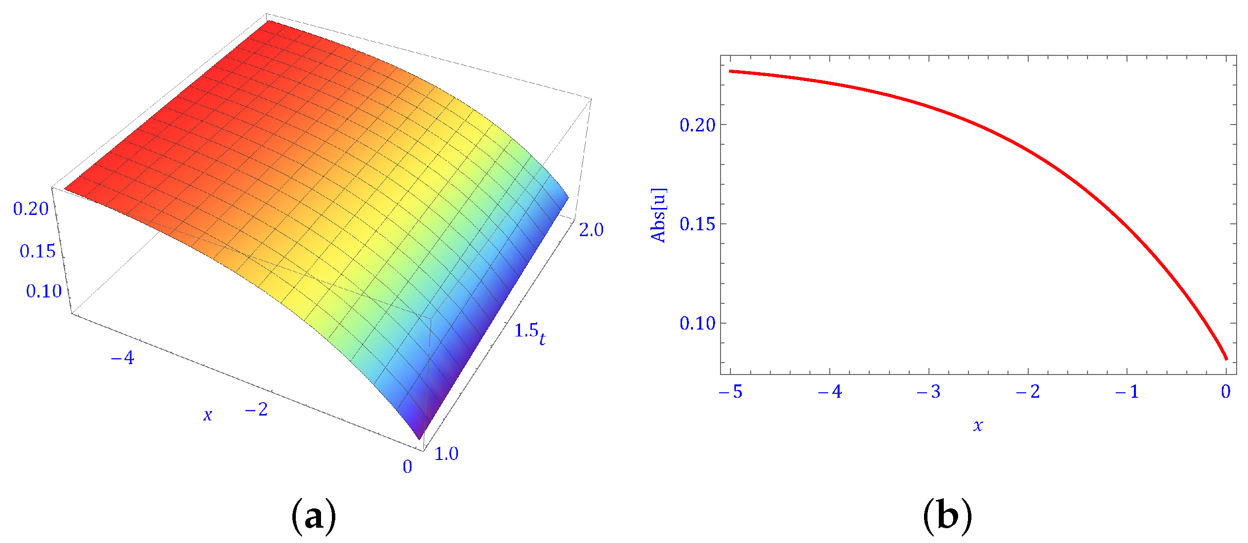
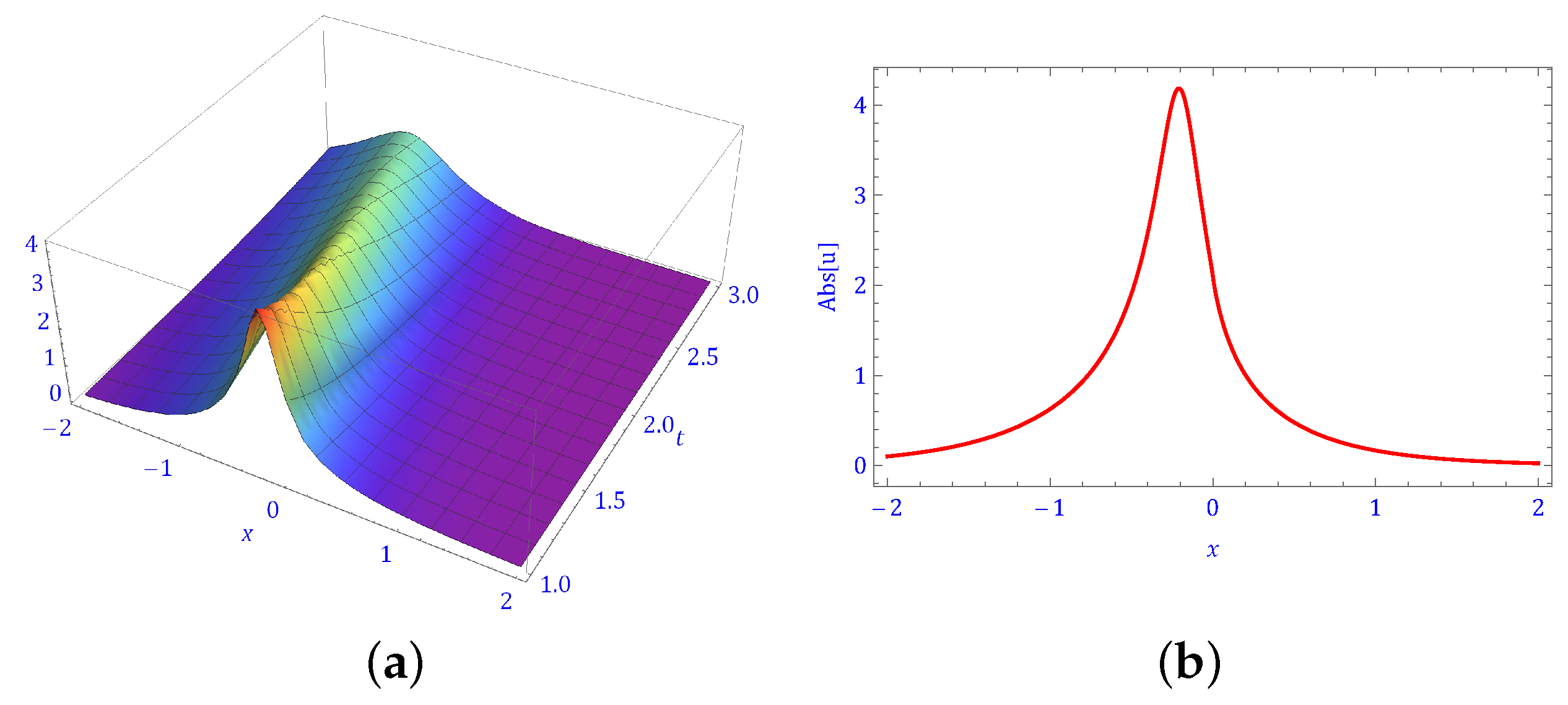
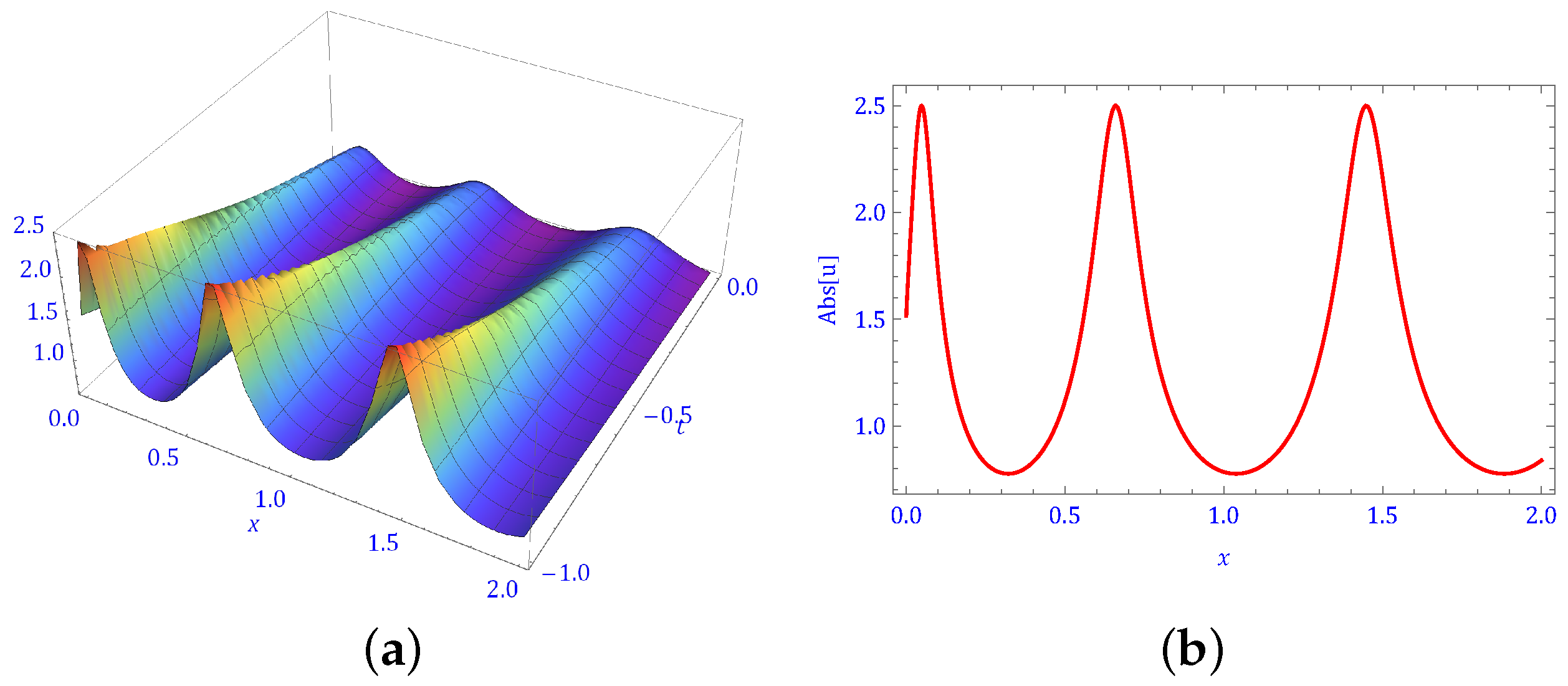
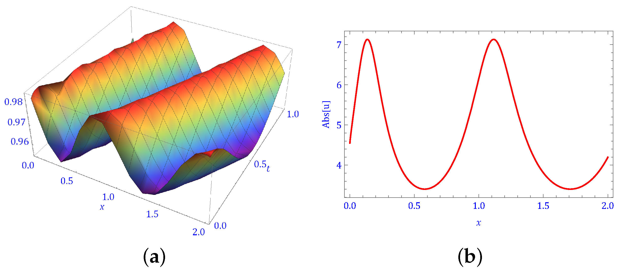
5. Physical Behavior of Solutions

This portion includes the representations of the physical behavior of the soliton solutions by using MATHEMATICA software, like kink type behavior of $u(x,y,t)$ that appears in Equation (23), is shown in Figure 1, where 3-dimensional and 2-dimensional plots are shown in Figure 1a and Figure 1b respectively for $d=2; {\beta }_0=0.5;{\beta }_1=0.4;$${\rm Y}=1; \tau =-0.5; \theta =0.5; \delta =1; y=-0.2; \alpha =0.9$; bright type behavior of $u(x,y,t)$ that appears in Equation (28), is shown in Figure 2, where 3-dimensional and 2-dimensional plots are shown in Figure 2a and Figure 2b respectively for ${\rm Y}=1; \tau =-0.5; \theta =0.5; \delta =1; y=-0.2;$$\alpha =0.8; \rho =-1; \mathrm{\Omega }=-1$; bright type behavior of $u(x,y,t)$ that appears in Equation (29), is shown in Figure 3, where 3-dimensional and 2-dimensional plots are shown in Figure 3a and Figure 3b respectively for ${\rm Y}=1; \tau =-0.5; \theta =0.5; \delta =1; y=-0.2; \alpha =0.8; \rho =-2;$$\mathrm{\Omega }=-2$; periodic type behavior of $u(x,y,t)$ that appears in Equation (30), is shown in Figure 4, where 3-dimensional and 2-dimensional plots are shown in Figure 4a and Figure 4b respectively for ${\rm Y}=2; \tau =-0.5; \theta =0.5; \delta =1; y=-0.2; \alpha =0.8; \rho =1; \mathrm{\Omega }=1$; and periodic type behavior of $u(x,y,t)$ that appears in Equation (31), is shown in Figure 5, where 3-dimensional and 2-dimensional plots are shown in Figure 5a and Figure 5b respectively for ${\rm Y}=2; \tau =-0.5; \theta =1.5; \delta =0.1; y=-1;\alpha =0.8; \rho =0.5; \mathrm{\Omega }=0.5$.

6. Conclusions

This paper obtained distinct kink, bright, and periodic soliton solution types of exact wave solitons for a truncated M-fractional (2+1)-dimensional nonlinear Kadomtsev–Petviashvili-modified equal-width (KP-mEW) equation. Two effective methods, the ${exp}_a$ function method and the modified extended tanh function method, were utilized. The achieved solutions were verified with the use of Mathematica software by putting the solutions back into the concerned equation. The use of the fractional derivative provides us with very valuable results. Some of the gained results are shown in 2-D and 3-D graphs. The results are helpful in the future study of the concerned model. The gained results are useful in different fields of science and engineering, including matter-wave pulses, waves in ferromagnetic media, and long-wavelength water waves with frequency dispersion and faintly nonlinear reinstating forces. Both of these methods provide a variety of solutions. The methods applied are also simple and useful for other nonlinear fractional partial differential equations.

References

1. Seadawy, A.R.; Ali, A.; Bekir, A. Exact wave solutions of new generalized Bogoyavlensky–Konopelchenko model in fluid mechanics. Mod. Phys. Lett. B 2024, 38, 2450262. [Google Scholar] [CrossRef]
2. Kai, Y.; Yin, Z. Linear structure and soliton molecules of Sharma-Tasso-Olver-Burgers equation. Phys. Lett. A 2022, 452, 128430. [Google Scholar] [CrossRef]
3. Durur, H. Exact Solutions of the Oskolkov Equation in Fluid Dynamics. Afyon Kocatepe Üniversitesi Fen Ve Mühendislik Bilimleri Dergisi 2023, 23, 355–361. [Google Scholar] [CrossRef]
4. Zhou, Q.; Pan, A.; Mirhosseini-Alizamini, S.M.; Mirzazadeh, M.; Liu, W.; Biswas, A. Group analysis and exact soliton solutions to a new (3+1)-dimensional generalized Kadomtsev-Petviashvili equation in fluid mechanics. Acta Phys. Pol. A 2018, 134, 564–569. [Google Scholar] [CrossRef]
5. Ullah, M.S.; Abdeljabbar, A.; Roshid, H.-O.; Ali, M.Z. Application of the unified method to solve the Biswas–Arshed model. Results Phys. 2022, 42, 105946. [Google Scholar] [CrossRef]
6. Aydemir, T. Application of the generalized unified method to solve (2+1)-dimensional Kundu–Mukherjee–Naskar equation. Opt. Quantum Electron. 2023, 55, 534. [Google Scholar] [CrossRef]
7. Nikan, O.; Avazzadeh, Z.; Rasoulizadeh, M.N. Soliton wave solutions of nonlinear mathematical models in elastic rods and bistable surfaces. Eng. Anal. Bound. Elem. 2022, 143, 14–27. [Google Scholar] [CrossRef]
8. Kai, Y.; Ji, J.; Yin, Z. Study of the generalization of regularized long-wave equation. Nonlinear Dyn. 2022, 107, 2745–2752. [Google Scholar] [CrossRef]
9. Ma, W.-X.; Huang, Y.; Wang, F.; Zhang, Y.; Ding, L. Binary Darboux transformation of vector nonlocal reverse-space nonlinear Schrödinger equations. Int. J. Geom. Methods Mod. Phys. 2024, 2450182. [Google Scholar] [CrossRef]
10. Yang, J.Y.; Ma, W.X. Four-component Liouville integrable models and their bi-Hamiltonian formulations. Rom. J. Phys. 2024, 69, 101. [Google Scholar] [CrossRef]
11. Arnous, A.H.; Hashemi, M.S.; Nisar, K.S.; Shakeel, M.; Ahmad, J.; Ahmad, I.; Jan, R.; Ali, A.; Kapoor, M.; Shah, N.A. Investigating solitary wave solutions with enhanced algebraic method for new extended Sakovich equations in fluid dynamics. Results Phys. 2024, 57, 107369. [Google Scholar] [CrossRef]
12. Islam, S.M.R. Bifurcation analysis and exact wave solutions of the nano-ionic currents equation: Via two analytical techniques. Results Phys. 2024, 58, 107536. [Google Scholar] [CrossRef]
13. Zhu, C.; Al-Dossari, M.; Rezapour, S.; Shateyi, S. On the exact soliton solutions and different wave structures to the modified Schrödinger’s equation. Results Phys. 2023, 54, 107037. [Google Scholar] [CrossRef]
14. Zhu, C.; Abdallah, S.A.O.; Rezapour, S.; Shateyi, S. On new diverse variety analytical optical soliton solutions to the perturbed nonlinear Schrödinger equation. Results Phys. 2023, 54, 107046. [Google Scholar] [CrossRef]
15. Tala-Tebue, E.; Rezazadeh, H.; Djoufack, Z.I.; Eslam, M.; Kenfack-Jiotsa, A.; Bekir, A. Optical solutions of cold bosonic atoms in a zig-zag optical lattice. Opt. Quantum Electron. 2021, 53, 1–13. [Google Scholar] [CrossRef]
16. Raheel, M.; Zafar, A.; Tala-Tebue, E. Optical solitons to time-fractional Sasa-Satsuma higher-order non-linear Schrödinger equation via three analytical techniques. Opt. Quantum Electron. 2023, 55, 307. [Google Scholar] [CrossRef]
17. Zafar, A.; Ali, K.K.; Raheel, M.; Nisar, K.S.; Bekir, A. Abundant M-fractional optical solitons to the pertubed Gerdjikov–Ivanov equation treating the mathematical nonlinear optics. Opt. Quantum Electron. 2022, 54, 25. [Google Scholar] [CrossRef]
18. Hussein, H.H.; Ahmed, H.M.; Alexan, W. Analytical soliton solutions for cubic-quartic perturbations of the Lakshmanan-Porsezian-Daniel equation using the modified extended tanh function method. Ain Shams Eng. J. 2024, 15, 102513. [Google Scholar] [CrossRef]
19. Akbulut, A.; Taşcan, F. Application of conservation theorem and modified extended tanh-function method to (1+1)-dimensional nonlinear coupled Klein–Gordon–Zakharov equation. Chaos Solitons Fractals 2017, 104, 33–40. [Google Scholar] [CrossRef]
20. Islam, M.T.; Akter, M.A.; Gómez-Aguilar, J.F.; Akbar, M.A.; Torres-Jiménez, J. A novel study of the nonlinear Kadomtsev–Petviashvili-modified equal width equation describing the behavior of solitons. Opt. Quantum Electron. 2022, 54, 725. [Google Scholar] [CrossRef]
21. Islam, M.T.; Akter, M.A.; Ryehan, S.; Gómez-Aguilar, J.F.; Akbar, M.A. A variety of solitons on the oceans exposed by the Kadomtsev Petviashvili-modified equal width equation adopting different techniques. J. Ocean Eng. Sci. 2022; in press. [Google Scholar]
22. Ali, A.T.; Hassan, E.R. General expa-function method for nonlinear evolution equations. Appl. Math. Comput. 2010, 217, 451–459. [Google Scholar] [CrossRef]
23. Zayed, E.M.E.; Al-Nowehy, A.G. Generalized kudryashov method and general expa function method for solving a high order nonlinear schrödinger equation. J. Space Explor. 2017, 6, 1–26. [Google Scholar]
24. Hosseini, K.; Ayati, Z.; Ansari, R. New exact solutions of the Tzitzéica-type equations in non-linear optics using the expa function method. J. Mod. Opt. 2018, 65, 847–851. [Google Scholar] [CrossRef]
25. Zafar, A. The expa function method and the conformable time-fractional KdV equations. Nonlinear Eng. 2019, 8, 728–732. [Google Scholar] [CrossRef]
26. Ma, W.-X.; Fuchssteiner, B. Explicit and exact solutions to a Kolmogorov-Petrovskii-Piskunov equation. Int. J. Non-Linear Mech. 1996, 31, 329–338. [Google Scholar] [CrossRef]
27. Sulaiman, T.A.; Yel, G.; Bulut, H. M-fractional solitons and periodic wave solutions to the Hirota- Maccari system. Mod. Phys. Lett. B 2019, 33, 1950052. [Google Scholar] [CrossRef]
28. Sousa, J.V.D.C.; de Oliveira, E.C. A new truncated M-fractional derivative type unifying some fractional derivative types with classical properties. Int. J. Anal. Appl. 2018, 16, 83–96. [Google Scholar]
29. Wazwaz, A.M. The tanh method and the sine–cosine method for solving the KP-MEW equation. Int. J. Comput. Math. 2005, 82, 235–246. [Google Scholar] [CrossRef]
Figure 1. Plots for u ( x , y , t ) appearing in Equation (23) in (a) 3-dimensional and (b) 2-dimensional for d = 2 ;   β 0 = 0.5 ;   β 1 = 0.4 ;   Υ = 1 ;   τ = 0.5 ;   θ = 0.5 ;   δ = 1 ;   y = 0.2 ;   α = 0.9 .
Fractalfract 08 00442 g001
Figure 2. Plots for u ( x , y , t ) appearing in Equation (28) in (a) 3-dimensional and (b) 2-dimensional with Υ = 1 ;   τ = 0.5 ;   θ = 0.5 ;   δ = 1 ;   y = 0.2 ;   α = 0.9 ;   ρ = 1 ;   Ω = 1 .
Fractalfract 08 00442 g002
Figure 3. Plots for u ( x , y , t ) appearing in Equation (29) in (a) 3-dimensional and (b) 2-dimensional with Υ = 1 ;   τ = 0.5 ;   θ = 0.5 ;   δ = 1 ;   y = 0.2 ;   α = 0.8 ;   ρ = 2 ;   Ω = 2 .
Fractalfract 08 00442 g003
Figure 4. Plots for u ( x , y , t ) appearing in Equation (30) in (a) 3-dimensional and (b) 2-dimensional with Υ = 2 ;   τ = 0.5 ;   θ = 0.5 ;   δ = 1 ;   y = 0.2 ;   α = 0.8 ;   ρ = 1 ;   Ω = 1 .
Fractalfract 08 00442 g004
Figure 5. Plots for u ( x , y , t ) appearing in Equation (31) in (a) 3-dimensional and (b) 2-dimensional with Υ = 2 ;   τ = 0.5 ;   θ = 1.5 ;   δ = 0.1 ;   y = 1 ;   α = 0.8 ;   ρ = 0.5 ;   Ω = 0.5 .
Fractalfract 08 00442 g005
Disclaimer/Publisher’s Note: The statements, opinions and data contained in all publications are solely those of the individual author(s) and contributor(s) and not of MDPI and/or the editor(s). MDPI and/or the editor(s) disclaim responsibility for any injury to people or property resulting from any ideas, methods, instructions or products referred to in the content.