PQMLE and Generalized F-Test of Random Effects Semiparametric Model with Serially and Spatially Correlated Nonseparable Error

Abstract

Semiparametric panel data models are powerful tools for analyzing data with complex characteristics such as linearity and nonlinearity of covariates. This study aims to investigate the estimation and testing of a random effects semiparametric model (RESPM) with serially and spatially correlated nonseparable error, utilizing a combination of profile quasi-maximum likelihood estimation and local linear approximation. Profile quasi-maximum likelihood estimators (PQMLEs) for unknowns and a generalized F-test statistic $F_{NT}$ are built to determine the beingness of nonlinear relationships. The asymptotic properties of PQMLEs and $F_{NT}$ are proven under regular assumptions. The Monte Carlo results imply that the PQMLEs and $F_{NT}$ performances are excellent on finite samples; however, missing the spatially and serially correlated error leads to estimator inefficiency and bias. Indonesian rice-farming data is used to illustrate the proposed approach, and indicates that $landarea$ exhibits a significant nonlinear relationship with $riceyield$, in addition, $high$-$yieldvarieties$, $mixed$-$yield$$varieties$, and $seedweight$ have significant positive impacts on rice yield.

1. Introduction

By tracking each individual in a predetermined sample over time, a panel dataset with multiple observations can be collected. In contrast to cross-sectional data (Cheng and Chen [1]), the panel data structure is sufficiently abundant to permit estimation and testing of regression models that include not only individual characteristics observed by the researchers but also unobserved characteristics that vary across individuals or/and time periods, simply referred to as “individual or/and time effects”. In recent decades, many studies have focused on parametric panel data models (Chamberlain [2], Chamberlain [3], Hsiao [4], Baltagi [5], Arellano [6], Wooldridge [7], Thapa et al. [8], and Rehfeldt and Weiss [9]).

In practice, a lot of spatial panel datasets are collected from “locations” and require further studying. Therefore, based on classic parametric panel data models, different types of parametric panel data models with spatial correlations at different locations are presented. There are three fundamental types of spatial parametric panel data model (Elhorst [10]): spatial autoregressive (SAR) model (Brueckner [11]), spatial Durbin model (SDM) (LeSage [12], Elhorst [13]), and spatial error model (SEM) (Allers and Elhorst [14]). A more detailed discussion can be found in Elhorst [15], Baltagi and Li [16], Pesaran [17], Kapoor et al. [18], Lee and Yu [19], Mutl and Pfaffermayr [20], and Baltagi et al. [21]. Among these, the SEM introduced by Anselin [22] accounts for the interaction effects in spatially correlated determinants of the dependent variable that is excluded from the model or in unobserved shocks with a spatial mode (Elhorst [13]). The development of testing and estimation of SEM has been summarized in books by Baltagi [5], Elhorst [10], and Anselin [22] as well as in surveys by Baltagi et al. [23], Bordignon et al. [24], and Kelejian and Prucha [25], among others. However, the aforementioned SEM assumes that the only correlation over time results from the same regional impact presented across the panel. In spatial panel data analysis, this assumption may be too restrictive for real situations. For example, if an undetected shock influences investments across regions, behavioral relationships are affected, at least in the next few stages. Thus, ignoring serially correlated errors may lead to inefficient regression coefficient estimators (Baltagi [5]).

By adding serially correlated errors to SEM, parametric panel data models with serially and spatially correlated errors can be established. The extended models consider not only serial correlations through spatial units but also spatial correlations at every point temporally. Researchers have established two types of parametric panel data models with serially and spatially correlated separable and nonseparable errors. The model with the separable error was used to analyze the effects of public infrastructure investment on the costs and productivity of private enterprises (Cohen and Paul [26]). The MLE and corresponding asymptotic properties of spatial panel data model with serially and spatially correlated separable error were investigated by Lee and Yu [27]. A random effects parametric panel data model with serially and spatially correlated error was introduced by Parent and LeSage [28], and the estimators were obtained using the Markov chain Monte Carlo (MCMC) method. Elhorst [29] constructed the MLE of a parametric panel data model with serially and spatially correlated nonseparable error without establishing the asymptotic properties of the estimators. Lee and Yu [30] established the QMLE and corresponding asymptotic properties for both linear panel data models with serially and spatially correlated separable and nonseparable errors.

Although the theories and applications of the aforementioned linear parametric panel data models with serially and spatially correlated separable/nonseparable errors have been thoroughly explored, their usefulness in applications is often impractical because they lack flexibility and are limited in their ability to detect complicated structures (e.g., nonlinearity). Furthermore, a misspecification of the data generating process by the linear parametric panel data model may result in significant modeling bias and can lead to incorrect findings. For these reasons, Zhao et al. [31] investigated the estimation and testing issues of a partially linear single-index panel data model with serially and spatially correlated separable errors using the semiparametric minimum average variance method and a F-type test statistic. Li et al. [32] obtained the PQMLE, the generalized F-test, and the asymptotic properties for a partially linear nonparametric regression model with serially and spatially correlated separable error. Li et al. [33] studied the PQMLEs of the unknowns for the fixed effects partially linear varying coefficient panel data model with serially and spatially correlated nonseparable error, thereby deriving the consistency and asymptotic normality. Bai et al. [34] constructed the estimators of the parametric and nonparametric components of a partially linear varying-coefficient panel data model with serially and spatially correlated separable errors using weighted semiparametric least squares and weighted polynomial spline series methods, respectively, thereby proving their asymptotic normality.

By adding a nonparametric component to a random effects parametric model with serially and spatially correlated nonseparable errors, a new random effects semiparametric model (RESPM) can be established to concurrently capture the linearity and nonlinearity of the covariates, spatial correlation and serial correlation of errors, and individual random effects. This study explores its PQMLE and hypothesis testing issues from theoretical, simulation, and application perspectives. Our proposed model is different from the model proposed by Li et al. [32], which assumes spatially and serially correlated errors are separable. The difference in model structure leads to differences in the following aspects: (1) The parameter spaces (i.e, stationarity conditions) of the two models are different. (2) There are differences in the estimation process, assumption conditions and theorem proofs.

The remainder of this paper is organized as follows: In Section 2, a RESPM with serially and spatially correlated nonseparable error is introduced, and the estimation and testing procedures are established. Section 3 lists several regular assumptions and theorems for the estimators and test statistic. In Section 4 and Section 5, numerical simulations and real data analyses are presented. Finally, Section 6 summarizes the results. The Appendix contains the proofs of the lemmas and theorems.

Notation. Some important symbols and their definitions that appear throughout the paper are given in Table 1.

Table 1. Some important symbols and their definitions.

Symbol	Definition
${\omega }_{max}$	Maximum eigenvalue of matrix W
${\omega }_{min}$	Minimum eigenvalue of matrix W
$\left|\rho \right|$	The absolute value of $\rho$
$|\mathrm{\Sigma }|$	The determinant of matrix $\mathrm{\Sigma }$
${\mathrm{\Sigma }}^{\prime }$	The transpose of matrix $\mathrm{\Sigma }$
${\mathrm{\Sigma }}^{-1}$	The inverse of matrix $\mathrm{\Sigma }$
$tr(\mathrm{\Sigma })$	The Trace of matrix $\mathrm{\Sigma }$
$diag(a_1,\cdots ,a_n)$	Diagonal matrix composed of elements $a_1,\cdots ,a_n$
$\parallel S\parallel$	${tr\left(S^{\prime }S\right)}^{\frac{1}{2}}=\{{\sum }_{ij}|s_{ij}{{|}^2\}}^{\frac{1}{2}}$
$\stackrel{D}{⟶}$	Convergence in distribution
$\stackrel{P}{⟶}$	Convergence in probability
$iid$	Independent idetically distributed
$K\ast K$	The convolution of function K
⊗	Kronecker product
≡	”Defined as” or “marked as”
$\mathcal{N}(0,\mathrm{\Sigma })$	Normal distribution with mean 0 and variance $\mathrm{\Sigma }$
${\chi }_{df}^2$	${\chi }^2$ distribution with degree of freedom $df$

2. Estimation and Testing

2.1. The Model

The form of RESPM with serially and spatially correlated nonseparable errors is as follows:

$$y_{it}=z_{it}^{\prime }\gamma +f\left({\iota }_{it}\right)+b_i+{\nu }_{it},$$

(1)

where $i(1\le i\le N)$ denotes the i-th spatial unit; $t(1\le t\le T)$ denotes the t-th period; $y_{it}$ denotes the observation of the response variable; $z_{it}={(z_{it1},z_{it2},\dots ,z_{itp})}^{\prime }$ and ${\iota }_{it}={({\iota }_{it1},{\iota }_{it2},\dots ,{\iota }_{itq})}^{\prime }$ denote observations of p- and q-dimensional covariates, respectively; $\gamma ={({\gamma }_1,{\gamma }_2,\dots ,{\gamma }_p)}^{\prime }$ is a p-dimensional regression coefficient vector of $z_{it}$; $f(·)$ is an unknown nonparameteric function; $b_i$ represents the i-th individual random effect; and ${\nu }_{it}$ represents the it-th error term and is independent of $b_i$.

Let $Y_t={(y_{1t},\dots ,y_{Nt})}^{\prime }$, $Z_t={(z_{1t},\dots ,z_{Nt})}^{\prime }$, $F_t={(f\left({\iota }_{1t}\right),\dots ,f\left({\iota }_{Nt}\right))}^{\prime }$, and $b={(b_1,\dots ,b_N)}^{\prime }$. Then, model (1) can be expressed in the following matrix form

$$Y_t=Z_t\gamma +F_t+b+{\nu }_t,$$

(2)

and its error term follows a serially and spatially correlated nonseparable error structure.

$${\nu }_t={\rho }_{1}W{\nu }_t+{\rho }_2{\nu }_{t-1}+{ϵ}_t,$$

(3)

where ${\nu }_t={({\nu }_{1t},\dots ,{\nu }_{Nt})}^{\prime }$ and $W={\left(w_{ij}\right)}_{N\times N}$ is predetermined spatial weights matrix; ${ϵ}_t={({ϵ}_{1t},\dots ,{ϵ}_{Nt})}^{\prime }$, ${ϵ}_{it}\sim IID(0,{\xi }_{ϵ}^2)$, and $b_i\sim IID(0,{\xi }_b^2)$, ${\xi }_{ϵ}^2$, ${\xi }_b^2$ are the variances of ${ϵ}_{it}$ and $b_i$, respectively; and ${\rho }_1$ and ${\rho }_2$ denote the spatial and serial correlation coefficients, respectively. Similar to Elhorst [29], model stationarity requires not only $|{\rho }_2| < 1$ and $1/{\omega }_{min}<{\rho }_1<1/{\omega }_{max}$ but also

$$\left\{\begin{array}{cc}\hfill |{\rho }_2|& \hfill <1-{\rho }_1{\omega }_{max},if{\rho }_1\ge 0\hfill \\ \hfill |{\rho }_2|& \hfill >1-{\rho }_1{\omega }_{min},if{\rho }_1<0\hfill \end{array}\right.$$

where ${\omega }_{max}$ and ${\omega }_{min}$ denote the largest and smallest eigenvalues of W, respectively. Furthermore, let ${\delta }_0={({\rho }_{10},{\rho }_{20},{\gamma }_0^{\prime },{\xi }_{ϵ0}^2,{\xi }_{b0}^2)}^{\prime }$ be the true values of $\delta ={({\rho }_1,{\rho }_2,{\gamma }^{\prime },{\xi }_{ϵ}^2,{\xi }_b^2)}^{\prime }$; $f_0\left(\iota \right)$ is the true value of $f\left(\iota \right)$.

2.2. PQMLE

To ensure homogeneity of variance, (3) can be rewritten as

$$C{\nu }_t={\rho }_2{\nu }_{t-1}+{\nu }_t,$$

(4)

where $C=C\left({\rho }_1\right)\equiv I_N-{\rho }_{1}W$, $I_N$ denotes an $N\times N$ identity matrix. By repeated substitution, we obtain the following equation: $C{\nu }_t={\nu }_t+{\rho }_2{C}^{-1}{\nu }_{t-1}+{\rho }_2^2{C}^{-2}{\nu }_{t-2}+\dots$ because C is nonsingular. Therefore, $E\left(C{\nu }_t\right)=0$, and the variance of $C{\nu }_t$ is

$$\begin{array}{ll}Var\left(C{\nu }_t\right)& =E\left({\nu }_t{\nu }_t^{\prime }\right)+{\rho }_2^2{C}^{-1}E\left({\nu }_{t-1}{\nu }_{t-1}^{\prime }\right)C^{\prime -1}+{\rho }_2^4{C}^{-2}E\left({\nu }_{t-2}{\nu }_{t-2}^{\prime }\right)C^{\prime -2}+\dots \\ & ={\xi }_{ϵ}^2(I_N+{\rho }_2^2{C}^{-1}{C}^{\prime -1}+{\rho }_2^4{C}^{-2}{C}^{\prime -2}+\dots )\\ & ={\xi }_{ϵ}^2{[I_N-{\rho }_2^2{\left(C^{\prime }C\right)}^{-1}]}^{-1}.\end{array}$$

(5)

Substituting ${\nu }_t+b=Y_t-F_t-Z_t\gamma$ and ${\nu }_{t-1}+b=Y_{t-1}-F_{t-1}-Z_{t-1}\gamma$ into (3), we obtain

$$C{Y}_t=C(F_t+Z_t\gamma )+{\rho }_2(Y_{t-1}-F_{t-1}-Z_{t-1}\gamma )+{ϵ}_t+b,t>1.$$

Because $E\left({\nu }_t\right)=0$ and $Var\left({\nu }_t\right)={\xi }_{ϵ}^2{C}^{-1}{[I_N-{\rho }_2^2{\left(C^{\prime }C\right)}^{-1}]}^{-1}{C}^{\prime -1}$, model (2) for the first period of $Y_t$ can be written as

$${\mathrm{\Gamma }}^{1/2}C{Y}_1={\mathrm{\Gamma }}^{1/2}C{F}_1+{\mathrm{\Gamma }}^{1/2}C{Z}_1\gamma +{\mathrm{\Gamma }}^{1/2}CUb+{ϵ}_1+b,$$

where $\mathrm{\Gamma }=I_N-{\rho }_2^2{\left(C^{\prime }C\right)}^{-1}$ and ${\mathrm{\Gamma }}^{1/2}$ may potentially be the Cholesky or spectral decomposition of $\mathrm{\Gamma }$; $U=I_N\otimes l_T$, ⊗ denotes the Kronecker product. Letting ${\eta }_t={ϵ}_t+b$, then $\eta =Ub+ϵ$, and the covariance matrix of $\eta$ can be calculated as follows:

$$\mathrm{\Sigma }=Var(Ub+ϵ)={\xi }_{ϵ}^{2}I+{\xi }_b^2{I}_N\otimes \left(l_T{l}_T^{\prime }\right),|\mathrm{\Sigma }|={\xi }_{ϵ}^{2N(T-1)}{({\xi }_b^2+T{\xi }_{ϵ}^2)}^N,$$

$${\mathrm{\Sigma }}^{-1}=\frac{1}{{\xi }_{ϵ}^2}I+(\frac{1}{{\xi }_{ϵ}^2+T{\xi }_b^2}-\frac{1}{T{\xi }_b^2})I_N\otimes \left(\frac{1}{T}{l}_T{l}_T^{\prime }\right),$$

where $\eta ={({\eta }_1,\dots ,{\eta }_T)}^{\prime }$ and $ϵ={({ϵ}_1,\dots ,{ϵ}_T)}^{\prime }$; I denotes the $NT\times NT$ identity matrix; and $l_T$ is a T-dimensional vector consisting of ones. Hence, the log quasi-likelihood function of the proposed model is obtained as follows:

$$\begin{array}{ll}logL\left(\delta \right)=& -\frac{NT}{2}log\left(2\pi \right)+\frac{1}{2}log|\mathrm{\Gamma }|+Tlog\left|C\right|-\frac{N(T-1)}{2}log{\xi }_{ϵ}^2-\frac{N}{2}log({\xi }_{ϵ}^2+T{\xi }_b^2)\\ & -\frac{{\sum }_{t=2}^T{[C(Y_t-Z_t\gamma -F_t)-{\rho }_2(Y_{t-1}-Z_{t-1}\gamma -F_{t-1})]}^{\prime }H[C(Y_t-Z_t\gamma -F_t)-{\rho }_2(Y_{t-1}-Z_{t-1}\gamma -F_{t-1})]}{2({\xi }_{ϵ}^2+T{\xi }_b^2)}\\ & -\frac{{\sum }_{t=2}^T{[C(Y_t-Z_t\gamma -F_t)-{\rho }_2(Y_{t-1}-Z_{t-1}\gamma -F_{t-1})]}^{\prime }(I-H)[C(Y_t-Z_t\gamma -F_t)-{\rho }_2(Y_{t-1}-Z_{t-1}\gamma -F_{t-1})]}{2{\xi }_{ϵ}^2}\\ & -\frac{{(Y_1-Z_1\gamma -F_1)}^{\prime }{C}^{\prime }{{\mathrm{\Gamma }}^{1/2}}^{\prime }(I-H){\mathrm{\Gamma }}^{1/2}C(Y_1-Z_1\gamma -F_1)}{2{\xi }_{ϵ}^2}-\frac{{(Y_1-Z_1\gamma -F_1)}^{\prime }{C}^{\prime }{{\mathrm{\Gamma }}^{1/2}}^{\prime }H{\mathrm{\Gamma }}^{1/2}C(Y_1-Z_1\gamma -F_1)}{2({\xi }_{ϵ}^2+T{\xi }_b^2)},\end{array}$$

(6)

where $H=I_N\otimes \left(T^{-1}{l}_T{l}_T^{\prime }\right).$

Because $F_t$ is unknown, Equation (6) cannot be maximized to obtain the quasi-maximum likelihood estimators of the unknowns. To solve this issue, the unknowns of the model are estimated by combining PQMLE and Working Independence Theory (Cai [35]). The primary steps are as follows:

Step 1. Let ${\widehat{f}}_{IN}\left(\iota \right)$ be the initial estimator of $f\left(\iota \right)$. We further assume that $\gamma$ is known and let ${\widehat{f}}_{IN}\left(\iota \right)={\widehat{a}}_1$. Then, $\widehat{\varphi }={({\widehat{a}}_1,{\left(S{\widehat{a}}_2\right)}^{\prime })}^{\prime }$ can be obtained as

$$\widehat{\varphi }=\underset{a_1,a_2}{argmin}\frac{1}{NT}{[\tilde{Y}-\overrightarrow{\mathit{\iota }}\left(\iota \right)\varphi ]}^{\prime }{K}_S\left(\iota \right)[\tilde{Y}-\overrightarrow{\mathit{\iota }}\left(\iota \right)\varphi ],$$

where $a_2$ is the first derivative of $f\left(\iota \right)$, $\tilde{Y}={({\tilde{y}}_{11},\dots ,{\tilde{y}}_{1T},\dots ,{\tilde{y}}_{N1},\dots ,{\tilde{y}}_{NT})}^{\prime }$, ${\tilde{y}}_{it}=y_{it}-z_{it}^{\prime }\gamma$, $\overrightarrow{\mathit{\iota }}\left(\iota \right)={[{\mathit{\iota }}_{11}\left(\iota \right),\dots ,{\mathit{\iota }}_{1T}\left(\iota \right),\dots ,{\mathit{\iota }}_{N1}\left(\iota \right),\dots ,{\mathit{\iota }}_{NT}\left(\iota \right)]}^{\prime }$, ${\mathit{\iota }}_{it}\left(\iota \right)={[1,{S^{-1}({\iota }_{it}-\iota )}^{\prime }]}^{\prime }$; $\left|S\right|$ is the determinant of $S=diag(s_1,\dots ,s_q)$, $K_S\left(\iota \right)=diag[k_S({\iota }_{11}-\iota ),\dots ,k_S({\iota }_{1T}-\iota ),\dots ,k_S({\iota }_{N1}-\iota ),\dots ,k_S({\iota }_{NT}-\iota )],$ $k_S\left(\iota \right)={\left|S\right|}^{-1}k\left(S^{-1}\iota \right)$; and $k(·)$ is a q-dimensional kernel function.

Let $\mathit{\iota }\left(\iota \right)={\left[{\overrightarrow{\mathit{\iota }}}^{\prime }\left(\iota \right)K_S\left(\iota \right)\overrightarrow{\mathit{\iota }}\left(\iota \right)\right]}^{-1}{\overrightarrow{\mathit{\iota }}}^{\prime }\left(\iota \right)K_S\left(\iota \right)$, then $\widehat{\varphi }=\mathit{\iota }\left(\iota \right)\tilde{Y}$ and

$${\widehat{f}}_{IN}\left(\iota \right)={\mathit{\iota }}_e^{\prime }\left(\iota \right)\tilde{Y},$$

(7)

where ${\mathit{\iota }}_e\left(\iota \right)=e_0^{\prime }\mathit{\iota }\left(\iota \right)$, $e_0={(1,0,\dots ,0)}^{\prime }$.

Step 2. Denote $Y_1^{\ast }={\mathrm{\Gamma }}^{1/2}C(Y_1-{\mathit{\iota }}_{e,1}Y),Z_1^{\ast }={\mathrm{\Gamma }}^{1/2}C(Z_1-{\mathit{\iota }}_{e,1}Z)$, $Y_t^{\ast }=C(Y_t-{\mathit{\iota }}_{e,t}Y)-{\rho }_2(Y_{t-1}-{\mathit{\iota }}_{e,t-1}Y),Z_t^{\ast }=C(Z_t-{\mathit{\iota }}_{e,t}Z)-{\rho }_2(Z_{t-1}-{\mathit{\iota }}_{e,t-1}Z),$ where ${\mathit{\iota }}_{e,t}$ is an $N\times NT$ block of ${\mathit{\iota }}_e\left(\iota \right)$ in Equation (7) and $t>2$. Substituting ${\widehat{f}}_{IN}\left(\iota \right)$ into (6), we obtain

$$\begin{array}{ll}logL(\delta ,{\widehat{f}}_{IN}\left(\iota \right))=& -\frac{1}{2}log|\mathrm{\Gamma }|+Tlog\left|C\right|-\frac{N(T-1)}{2}log{\xi }_{ϵ}^2-\frac{N}{2}log({\xi }_{ϵ}^2+T{\xi }_b^2)\\ & -\frac{{(Y^{\ast }-Z^{\ast }\gamma )}^{\prime }H(Y^{\ast }-Z^{\ast }\gamma )}{2{\xi }_{ϵ}^2}-\frac{{(Y^{\ast }-Z^{\ast }\gamma )}^{\prime }(I-H)(Y^{\ast }-Z^{\ast }\gamma )}{2({\xi }_{ϵ}^2+T{\xi }_b^2)},\end{array}$$

(8)

where $Y^{\ast }={(Y_1^{{\ast }^{\prime }},\dots ,Y_T^{{\ast }^{\prime }})}^{\prime }$, $Z^{\ast }={(Z_1^{{\ast }^{\prime }},\dots ,Z_T^{{\ast }^{\prime }})}^{\prime }$. Therefore, the initial estimators of $\gamma$, ${\xi }_{\xi }^2$, and ${\xi }_b^2$ are:

$${{\widehat{\xi }}^2}_{ϵIN}=\frac{1}{N(T-1)}{\tilde{Y}}^{{\ast }^{\prime }}(I-H){\tilde{Y}}^{\ast },$$

(9)

$${{\widehat{\xi }}^2}_{bIN}=\frac{1}{NT}{\tilde{Y}}^{{\ast }^{\prime }}H{\tilde{Y}}^{\ast }-\frac{1}{T}{\widehat{\xi }}_{ϵIN}^2,$$

(10)

$${\widehat{\gamma }}_{IN}={[Z^{{\ast }^{\prime }}(\frac{H}{{{\widehat{\xi }}^2}_{ϵIN}}+\frac{I-H}{{{\widehat{\xi }}^2}_{ϵIN}+T{{\widehat{\xi }}^2}_{bIN}})Z^{\ast }]}^{-1}{Z}^{{\ast }^{\prime }}(\frac{H}{{{\widehat{\xi }}^2}_{ϵIN}}+\frac{I-H}{{{\widehat{\xi }}^2}_{ϵIN}+T{{\widehat{\xi }}^2}_{bIN}})Y^{\ast },$$

(11)

where ${\tilde{Y}}^{\ast }={({\tilde{Y}}_1^{\ast },\dots ,{\tilde{Y}}_T^{\ast })}^{\prime }$, and ${\tilde{Y}}_t^{\ast }=Y_t^{\ast }-Z_t^{{\ast }^{\prime }}\gamma$.

Step 3. By substituting (9)–(11) into (8), the concentrated log quasi-likelihood function of ${\rho }_1$ and ${\rho }_2$ can be calculated as follows:

$$\begin{array}{cc}\hfill log\tilde{L}({\rho }_1,{\rho }_2)& \hfill =-\frac{1}{2}log|\mathrm{\Gamma }|+Tlog\left|C\right|-\frac{N(T-1)}{2}log{\widehat{\xi }}_{ϵIN}^2-\frac{N}{2}log({\widehat{\xi }}_{ϵIN}^2+T{\widehat{\xi }}_{bIN}^2).\hfill \end{array}$$

(12)

Because Equation (12) is a nonlinear function of ${\rho }_1$ and ${\rho }_2$, the corresponding estimators obtained by the optimization algorithm are

$$({\widehat{\rho }}_1,{\widehat{\rho }}_2)=\underset{{\rho }_1,{\rho }_2}{argmax}log\tilde{L}({\rho }_1,{\rho }_2).$$

(13)

Step 4. Substituting ${\widehat{\rho }}_1$ and ${\widehat{\rho }}_2$ into (9)–(11), we obtain the ultimate estimators of $\gamma$, ${\xi }_{ϵ}^2$, and ${\xi }_b^2$ as $\widehat{\gamma }$, ${\widehat{\xi }}_{ϵ}^2$, and ${\widehat{\xi }}_b^2$, respectively. By replacing $\widehat{\gamma }$, ${\widehat{\xi }}_{ϵ}^2$, and ${\widehat{\xi }}_b^2$ in (7), the ultimate estimator $\widehat{f}\left(\iota \right)$ of $f\left(\iota \right)$ are obtained. Hence,

$${\widehat{{\xi }_{ϵ}}}^2=\frac{1}{N(T-1)}{\widehat{\tilde{Y}}}^{{\ast }^{\prime }}(I-H){\widehat{\tilde{Y}}}^{\ast },$$

(14)

$${\widehat{{\xi }_b}}^2=\frac{1}{NT}{\widehat{\tilde{Y}}}^{{\ast }^{\prime }}H{\widehat{\tilde{Y}}}^{\ast }-\frac{1}{T}{\widehat{\xi }}_{ϵ}^2,$$

(15)

$$\widehat{\gamma }={[{\widehat{Z}}^{{\ast }^{\prime }}(\frac{H}{{\widehat{\xi }}_{ϵ}^2}+\frac{I-H}{{\widehat{\xi }}_{ϵ}^2+T{\widehat{\xi }}_b^2}){\widehat{Z}}^{\ast }]}^{-1}{\widehat{Z}}^{{\ast }^{\prime }}(\frac{H}{{\widehat{\xi }}_{ϵ}^2}+\frac{I-H}{{\widehat{\xi }}_{ϵ}^2+T{\widehat{\xi }}_b^2}){\widehat{Y}}^{\ast },$$

(16)

$$\widehat{f}\left(\iota \right)={\mathit{\iota }}_e^{\prime }\left(\iota \right)\widehat{\tilde{Y}},$$

(17)

where ${\widehat{\tilde{Y}}}^{\ast }={({\widehat{\tilde{Y}}}_1^{{\ast }^{\prime }},\dots ,{\widehat{\tilde{Y}}}_T^{{\ast }^{\prime }})}^{\prime }$, ${\widehat{\tilde{Y}}}_t^{\ast }={\widehat{Y}}_t^{\ast }-{\widehat{Z}}_t^{{\ast }^{\prime }}\widehat{\gamma }$, ${\widehat{Y}}^{\ast }={({\widehat{Y}}_1^{{\ast }^{\prime }},\dots ,{\widehat{Y}}_T^{{\ast }^{\prime }})}^{\prime }$, ${\widehat{Z}}^{\ast }={({\widehat{Z}}_1^{{\ast }^{\prime }},\dots ,{\widehat{Z}}_T^{{\ast }^{\prime }})}^{\prime }$,${\widehat{Y}}_1^{\ast }={\widehat{\mathrm{\Gamma }}}^{1/2}\widehat{C}(Y_1-{\mathit{\iota }}_{e,1}Y)$, ${\widehat{Z}}_1^{\ast }={\widehat{\mathrm{\Gamma }}}^{1/2}\widehat{C}(Z_1-{\mathit{\iota }}_{e,1}Z)$, ${\widehat{Y}}_t^{\ast }=\widehat{C}(Y_t-{\mathit{\iota }}_{e,t}Y)-{\widehat{\rho }}_2(Y_{t-1}-{\mathit{\iota }}_{e,t-1}Y)$, ${\widehat{Z}}_t^{\ast }=\widehat{C}(Z_t-{\mathit{\iota }}_{e,t}Z)-{\widehat{\rho }}_2(Z_{t-1}-{\mathit{\iota }}_{e,t-1}Z),$$\widehat{\mathrm{\Gamma }}=I_N-{\widehat{\rho }}_2^2{({\widehat{C}}^{\prime }\widehat{C})}^{-1}$, $\widehat{C}=I_N-{\widehat{\rho }}_{1}W$, and $\widehat{\tilde{Y}}=Y-Z^{\prime }\widehat{\gamma }$.

2.3. Hypothesis Test for Nonparametric Component

As outlined in Section 2.2, a hypothesis test is constructed to ensure the rationality of nonparametric model specification (1) as follows:

$$H_0:f\left({\iota }_{it}\right)={\zeta }_0+\sum _{j=1}^q{\zeta }_j{\iota }_{itj}versus{H}_1:f\left({\iota }_{it}\right)\ne {\zeta }_0+\sum _{j=1}^q{\zeta }_j{\iota }_{itj},$$

where ${\zeta }_0,{\zeta }_1,\dots ,{\zeta }_q$ are constant parameters. Following the generalized F-test statistic introduced by Fan et al. [36], let $\widehat{f}\left({\iota }_{it}\right)$ be the estimator obtained by the PQML method in Section 2.2. Let $\tilde{f}\left({\iota }_{it}\right)={\tilde{\zeta }}_0+{\sum }_{j=1}^q{\tilde{\zeta }}_j{\iota }_{itj}$ and $\tilde{\zeta }$ be the quasi-maximum likelihood estimators. The resulting residual sum of squares can be obtained using the null and alternative hypotheses, respectively:

$$\begin{array}{c}\hfill RSS\left(H_0\right)=\sum _i^N\sum _{t=1}^T{[y_{it}-\tilde{f}\left({\iota }_{it}\right)-z_{it}^{\prime }\tilde{\gamma }]}^2,\\ \hfill RSS\left(H_1\right)=\sum _i^N\sum _{t=1}^T{[y_{it}-\widehat{f}\left({\iota }_{it}\right)-z_{it}^{\prime }\widehat{\gamma }]}^2.\end{array}$$

To test the null hypothesis, a test statistic is conducted as follows:

$$F_{NT}=\frac{NT}{2}\frac{RSS\left(H_0\right)-RSS\left(H_1\right)}{RSS\left(H_1\right)}.$$

(18)

3. Asymptotic Theory

3.1. Assumptions

Before presenting the theoretical analysis of the proposed PQMLEs and test statistic, we make some regular assumptions.

Assumption 1.

(i) 

Covariates ${\{z_{it},{\iota }_{it}\}}_{i=1,t=1}^{N,T}$ are nonstochastic regressors which are uniformly bounded (UB) in $\mathcal{Z}\times \mathrm{\Delta }$, where $\mathcal{Z}$ and Δ are parameter spaces of $z_{it}$ and ${\iota }_{it}$, respectively.

(ii) 

There exist $m_t(·)$ and a continuous function $\epsilon (·)$ that satisfy $m_t(·)>0$ and $\underset{N\to \infty }{lim}\frac{1}{N}{\sum }_{i=1}^N\epsilon \left({\iota }_i\right)=\int \epsilon \left(\iota \right)m_t\left(\iota \right)d\iota$.

Assumption 2.

(i) 

$w_{ii}=0$, $w_{ij}=O(1/l_N)$, where $W={\left(w_{ij}\right)}_{N\times N}$.

(ii) 

When $N\to \infty$, $l_N/N\to 0$ holds.

(iii) 

C is nonsingular in parameter space Λ.

(iv) 

The row and column sums of W and $C^{-1}$ are UB.

Assumption 3.

As $N\to \infty$, $\parallel S\parallel \to 0$, ${N\left|S\right|}^2\to \infty$, ${\parallel S\parallel }^4{\left|S\right|}^{-1}\to 0$ and ${N\left|S\right|\parallel S\parallel }^4\to M\in [0,\infty )$, where M is a constant.

Assumption 4.

$K(·)$ is a kernel function on $R^q$ with 0 odd order moments.

Assumption 5.

The models (1)–(3) are tenable with ${\delta }_0={({\rho }_{10},{\rho }_{20},{\gamma }_0^{\prime },{\xi }_{ϵ0}^2,{\xi }_{b0}^2)}^{\prime }$.

Assumption 6.

${\mathrm{\Sigma }}_{{\delta }_0}$ is a positive definite matrix, as defined in Theorem 2.

Remark 1.

Assumption 1 provides the features of the covariates, random error term, and density function. Assumption 2 concerns the basic features of the spatial weights matrix parallels Assumption 3 in Su and Jin [37] and Assumption 5 in Lee [38]. Assumptions 3 and 4 are related to the bandwidth and kernel functions. Specifically, Assumption 3 is similar to Assumption 4 of Hamilton and Truong [39] and Assumption 7 of Su and Ullah [40] and is easily satisfied by considering $S=diag(s_1,...,s_q)$ with $s_i\propto N^{1/(4+q)}$ for $q<4$. Assumptions 5 and 6 are important for proving the consistency and asymptotic properties of the estimators.

3.2. Asymptotic Properties

The reduced form of $y_{it}$ is obtained as follows:

$$y_{it}=z_{it}^{\prime }{\gamma }_0+f_0\left({\iota }_{it}\right)+b_i+{\nu }_{it},$$

(19)

$${\nu }_{it}={\rho }_{10}\sum _{j=1}^N{w}_{ij}{\nu }_{jt}+{\rho }_{20}{\nu }_{i,t-1}+{ϵ}_{it}.$$

(20)

Note that ${\mathit{\iota }}_e=({\mathit{\iota }}_{e11},\dots ,{\mathit{\iota }}_{eNT})$, where ${\mathit{\iota }}_{eit}={\mathit{\iota }}_e\left({\mathit{\iota }}_{it}\right)$. Denote a typical entry of ${\mathit{\iota }}_e\left(\iota \right)$ by ${\mathit{\iota }}_e({\iota }_{it},\iota )=e^{\prime }{\left[{\overrightarrow{\mathit{\iota }}}^{\prime }\left(\iota \right)K_S\left(\iota \right)\overrightarrow{\mathit{\iota }}\left(\iota \right)\right]}^{-1}{\overrightarrow{\mathit{\iota }}}_{it}^{\prime }\left(\iota \right)K_S({\iota }_{it}-\iota )$, where ${\overrightarrow{\mathit{\iota }}}_{it}\left(\iota \right)$ is a typical column of $\overrightarrow{\mathit{\iota }}\left(\iota \right)$.

Lemma 1.

Upon fulfilling Assumptions 1–5, we have $\parallel \mathit{\iota }\parallel =O_p(N^{-1/2}{\left|S\right|}^{-1/2}).$

Hamilton and Truong [39] provided the proof.

Lemma 2.

Upon fulfilling Assumptions 1–5, we have

(i) 

${\mathit{\iota }}_e({\iota }_{it},\iota )=N^{-1}{K}_S({\iota }_{it}-\iota )\overline{m}\left(\iota \right)[1+op\left(1\right)]$, where $\overline{m}\left(\iota \right)={\sum }_{t=1}^T{m}_t\left(\iota \right)$.

(ii) 

$\underset{N\to \infty }{lim}P\{N^{-1}{\left[{\overrightarrow{\mathit{\iota }}}^{\prime }\left(\iota \right)K_S\left(\iota \right)\overrightarrow{\mathit{\iota }}\left(\iota \right)\right]}_{ij}\le M\}=1$ for $\iota \in \mathrm{\Delta },i,j=1,\dots ,q+1$.

(iii) 

$\underset{N\to \infty }{lim}P\{\underset{\iota }{sup}\underset{1\le i\le N,1\le t\le T}{max}|{\mathit{\iota }}_e({\iota }_{it},\iota )|\le O{\left(NT\right)}^{-1}{\left|S\right|}^{-1}\}=1$.

Su and Ullah [41] provided the proofs.

Lemma 3.

Upon fulfilling Assumptions 1–5, we have $\parallel (I-\iota ){\left(F_t\right)}_{NT\times NT}{\parallel =Op(\parallel S\parallel }^2).$

Hamilton and Truong [39] provided the proof.

Using the lemmas listed above, we establish the following theorems:

Theorem 1.

Fulfillment of Assumptions 1–5 leads to $\widehat{\delta }-{\delta }_0=o_p\left(1\right)$.

Theorem 2.

Fulfillment of Assumptions 1–6 leads to

$$\sqrt{NT}(\widehat{\delta }-{\delta }_0)\stackrel{D}{⟶}\mathcal{N}(0,\underset{N\to \infty }{lim}({\mathrm{\Sigma }}_{{\delta }_0}^{-1}+{\mathrm{\Sigma }}_{{\delta }_0}^{-1}{\mathrm{\Omega }}_{{\delta }_0}{\mathrm{\Sigma }}_{{\delta }_0}^{-1})),$$

where ${\mathrm{\Sigma }}_{{\delta }_0}=-E\left[\frac{1}{\sqrt{NT}}\frac{{\partial }^{2}logL\left({\delta }_0\right)}{\partial \delta \partial {\delta }^{\prime }}\right]$, ${\mathrm{\Omega }}_{{\delta }_0}$ is defined in (A7).

Theorem 3.

Fulfillment of Assumptions 1–4 leads to

$$\sqrt{N\left|S\right|}(\widehat{\varphi }-\varphi )\stackrel{D}{⟶}\mathcal{N}(0,{\sigma }^2\left(\varphi \right)),$$

where ${\sigma }^2\left(\varphi \right)={\acute{G}}^{\prime }{\mathit{\iota }}^{\prime }\left(\iota \right){\sigma }_{\eta }^2\mathit{\iota }\left(\iota \right)\acute{G}$ and the form of $\acute{G}$ is provided in the Appendix.

Theorem 4.

Fulfillment of Assumptions 1–4 leads to

$$r_k{F}_{NT}\stackrel{D}{⟶}{\chi }_{df}^2,$$

where $df=r_k{c}_k|\mathrm{\Delta }|/\left|S\right|,r_k=\frac{K\left(0\right)-\frac{1}{2}\int K^2\left(\iota \right)d\iota }{\int {(K\left(\iota \right)-\frac{1}{2}K\ast K\left(\iota \right))}^{2}d\iota },c_k=K\left(0\right)-\frac{1}{2}\int K^2\left(\iota \right)d\iota$, Δ is the support set of ι, $K\left(\iota \right)=diag(S^{-1}k\left(S^{-1}({\iota }_{11}-\iota )\right),\dots ,S^{-1}k\left(S^{-1}({\iota }_{NT}-\iota )\right))$.

Remark 2.

This paper focuses on the case with a large N and fixed T. In terms of estimation procedure, there is no restriction on N and T. Therefore, the estimation method can be applied to both fixed and large T cases. However, the asymptotic theory of estimators with both the fixed T and large T cases may be different.

4. Monte Carlo Simulation

4.1. Performance of PQMLEs

This section is devoted to use Monte Carlo simulation to examine the performance of PQMLEs in finite sample cases. The mean square error ($MSE$), mean absolute deviation error ($MADE$), and standard deviation ($SD$) are used as the evaluation criteria, where

$${\mathrm{MADE}}_j=Q^{-1}\sum _{q=1}^Q|\widehat{f}\left({\iota }_q\right)-f\left({\iota }_q\right)|,j=1,2,\cdots ,srt,$$

${\left\{{\iota }_q\right\}}_{q=1}^Q$ are fixed nodes in the support set of $\iota$, and $srt$ denotes the number of repetitions. In the subsequent simulations, $K\left(\iota \right)=\frac{3}{4\sqrt{5}}(1-\frac{1}{5}{\iota }^2)1({\iota }^2\le 5)$ (Su [42]) and the rule of thumb method (Mack and Silverman [43]) is utilized to select window width and srt is set as 1000.

The simulation data are generated using the following model:

$$\left\{\begin{array}{ll}{y}_{it}& =z_{it}^{\prime }\gamma +f\left({\iota }_{it}\right)+b_i+{\nu }_{it},\\ {\nu }_{it}& ={\rho }_1\sum _{j=1}^N{w}_{ij}{\nu }_{jt}+{\rho }_2{\nu }_{i,t-1}+{ϵ}_{it},i=1,\dots ,N,t=1,\dots ,T,\end{array}\right.$$

(21)

where N, T are the numbers of spatial unit and time period, respectively. In order to study the performance of PQMLEs in different finite sample cases, we take $N=40,60,80$ and $T=10,15,20$ respectively. $z_{it}\sim U[-2,2]$, ${\iota }_{it}\sim U[-3,3]$, $b_i\sim i.i.d.\mathcal{N}(0,0.5)$, ${ϵ}_{it}\sim i.i.d.\mathcal{N}(0,0.5)$, $f\left({\iota }_{it}\right)=sin(-\frac{1}{2}{\iota }_{it}^2)+0.6{\iota }_{it}+1$, $\gamma =1$, respectively. According to the parameter space of ${\rho }_1$ and ${\rho }_2$, we set ${\rho }_1=0.2,0.7$, and ${\rho }_2=0.4,0.5$, respectively. $W={\left(w_{ij}\right)}_{N\times N}$ is replaced with the Rook weights matrix (Anselin [22]). The simulation results are listed in Figure 1 and Table 2, Table 3, Table 4, Table 5, Table 6 and Table 7.

Figure 1. $\widehat{f}\left(\iota \right)$ and its 95% confidence intervals with ${\rho }_1=0.2$ and ${\rho }_2=0.7$ under different N and T.

Table 2. Parametric simulation results with N = 40.

			T = 10		T = 15		T = 20
	Parameter	True	Mean	MSE	Mean	MSE	Mean	MSE
	${\widehat{\rho }}_1$	0.2000	0.1746	0.0017	0.2113	0.0015	0.2046	0.0012
	${\widehat{\rho }}_2$	0.7000	0.7646	0.0014	0.6786	0.0009	0.6895	0.0007
${\rho }_1=0.2$	$\widehat{\gamma }$	1.6000	1.6034	0.0022	1.6010	0.0016	1.6008	0.0013
${\rho }_2=0.7$	$\widehat{{\xi }_{ϵ}^2}$	0.5000	0.4746	0.0346	0.4932	0.0214	0.5035	0.0075
	$\widehat{{\xi }_b^2}$	0.5000	0.5512	0.0154	0.5313	0.0045	0.5054	0.0014
	${\widehat{\rho }}_1$	0.4000	0.4279	0.0038	0.3870	0.0028	0.3889	0.0020
	${\widehat{\rho }}_2$	0.5000	0.5590	0.0029	0.5589	0.0025	0.5330	0.0019
${\rho }_1=0.4$	$\widehat{\gamma }$	1.6000	1.6005	0.0009	1.6003	0.0007	1.5998	0.0004
${\rho }_2=0.5$	$\widehat{{\xi }_{ϵ}^2}$	0.5000	0.5700	0.0242	0.5353	0.0212	0.5243	0.0205
	$\widehat{{\xi }_b^2}$	0.5000	0.5425	0.0351	0.5166	0.0138	0.5138	0.0108
	${\widehat{\rho }}_1$	0.5000	0.5287	0.0037	0.4722	0.0032	0.4869	0.0031
	${\widehat{\rho }}_2$	0.4000	0.4640	0.0031	0.4264	0.0030	0.4113	0.0028
${\rho }_1=0.5$	$\widehat{\gamma }$	1.6000	1.5981	0.0007	1.6005	0.0003	1.6004	0.0002
${\rho }_2=0.4$	$\widehat{{\xi }_{ϵ}^2}$	0.5000	0.5390	0.0176	0.5184	0.0141	0.4935	0.0034
	$\widehat{{\xi }_b^2}$	0.5000	0.5615	0.0177	0.4820	0.0119	0.5015	0.0039
	${\widehat{\rho }}_1$	0.7000	0.6667	0.0055	0.7092	0.0041	0.7054	0.0040
	${\widehat{\rho }}_2$	0.2000	0.2860	0.0052	0.2319	0.0043	0.2038	0.0037
${\rho }_1=0.7$	$\widehat{\gamma }$	1.6000	1.6020	0.0008	1.5996	0.0003	1.5997	0.0002
${\rho }_2=0.2$	$\widehat{{\xi }_{ϵ}^2}$	0.5000	0.5446	0.0051	0.5372	0.0024	0.5232	0.0014
	$\widehat{{\xi }_b^2}$	0.5000	0.5578	0.0152	0.5381	0.0091	0.5295	0.0027

Table 3. Parametric simulation results with N = 60.

			T = 10		T = 15		T = 20
	Parameter	True	Mean	MSE	Mean	MSE	Mean	MSE
	${\widehat{\rho }}_1$	0.2000	0.2130	0.0009	0.2081	0.0007	0.2007	0.0005
	${\widehat{\rho }}_2$	0.7000	0.7171	0.0016	0.6878	0.0014	0.6954	0.0004
${\rho }_1=0.2$	$\widehat{\gamma }$	1.6000	1.5981	0.0011	1.6006	0.0010	1.6002	0.0008
${\rho }_2=0.7$	$\widehat{{\xi }_{ϵ}^2}$	0.5000	0.4490	0.0287	0.4773	0.0213	0.5214	0.0057
	$\widehat{{\xi }_b^2}$	0.5000	0.5626	0.0074	0.5441	0.0071	0.4947	0.0069
	${\widehat{\rho }}_1$	0.4000	0.3912	0.0017	0.4074	0.0013	0.3949	0.0011
	${\widehat{\rho }}_2$	0.5000	0.5082	0.0018	0.5045	0.0015	0.5039	0.0012
${\rho }_1=0.4$	$\widehat{\gamma }$	1.6000	1.6007	0.0005	1.6004	0.0003	1.5999	0.0002
${\rho }_2=0.5$	$\widehat{{\xi }_{ϵ}^2}$	0.5000	0.5594	0.0205	0.4900	0.0200	0.5099	0.0195
	$\widehat{{\xi }_b^2}$	0.5000	0.4714	0.0090	0.4847	0.0087	0.5077	0.0079
	${\widehat{\rho }}_1$	0.5000	0.4730	0.0024	0.4823	0.0018	0.4858	0.0016
	${\widehat{\rho }}_2$	0.4000	0.4322	0.0022	0.4273	0.0017	0.4139	0.0014
${\rho }_1=0.5$	$\widehat{\gamma }$	1.6000	1.6005	0.0003	1.6003	0.0002	1.5998	0.0001
${\rho }_2=0.4$	$\widehat{{\xi }_{ϵ}^2}$	0.5000	0.5591	0.0071	0.5125	0.0065	0.5072	0.0026
	$\widehat{{\xi }_b^2}$	0.5000	0.4851	0.0118	0.4856	0.0103	0.5100	0.0030
	${\widehat{\rho }}_1$	0.7000	0.6808	0.0026	0.7130	0.0024	0.6876	0.0019
	${\widehat{\rho }}_2$	0.2000	0.2189	0.0025	0.2124	0.0023	0.1970	0.0016
${\rho }_1=0.7$	$\widehat{\gamma }$	1.6000	1.6010	0.0003	1.6008	0.0002	1.6007	0.0001
${\rho }_2=0.2$	$\widehat{{\xi }_{ϵ}^2}$	0.5000	0.5509	0.0035	0.5214	0.0020	0.5085	0.0012
	$\widehat{{\xi }_b^2}$	0.5000	0.5556	0.0086	0.5302	0.0084	0.5170	0.0019

Table 4. Parametric simulation results with N = 80.

			T = 10		T = 15		T = 20
	Parameter	True	Mean	MSE	Mean	MSE	Mean	MSE
	${\widehat{\rho }}_1$	0.2000	0.2066	0.0004	0.2048	0.0004	0.2003	0.0001
	${\widehat{\rho }}_2$	0.7000	0.6909	0.0006	0.6978	0.0003	0.6989	0.0002
${\rho }_1=0.2$	$\widehat{\gamma }$	1.6000	1.5991	0.0013	1.5997	0.0007	1.6002	0.0006
${\rho }_2=0.7$	$\widehat{{\xi }_{ϵ}^2}$	0.5000	0.4755	0.0079	0.5193	0.0047	0.4967	0.0046
	$\widehat{{\xi }_b^2}$	0.5000	0.5361	0.0063	0.5088	0.0061	0.5004	0.0039
	${\widehat{\rho }}_1$	0.4000	0.4012	0.0011	0.4004	0.0009	0.3999	0.0007
	${\widehat{\rho }}_2$	0.5000	0.5092	0.0010	0.5081	0.0008	0.5055	0.0007
${\rho }_1=0.4$	$\widehat{\gamma }$	1.6000	1.5986	0.0004	1.6010	0.0003	1.6003	0.0002
${\rho }_2=0.5$	$\widehat{{\xi }_{ϵ}^2}$	0.5000	0.4763	0.0204	0.4857	0.0157	0.4961	0.0097
	$\widehat{{\xi }_b^2}$	0.5000	0.5595	0.0087	0.4813	0.0074	0.4899	0.0068
	${\widehat{\rho }}_1$	0.5000	0.4933	0.0018	0.4997	0.0013	0.4998	0.0010
	${\widehat{\rho }}_2$	0.4000	0.4401	0.0017	0.4200	0.0014	0.4064	0.0013
${\rho }_1=0.5$	$\widehat{\gamma }$	1.6000	1.5991	0.0002	1.5994	0.0002	1.6002	0.0001
${\rho }_2=0.4$	$\widehat{{\xi }_{ϵ}^2}$	0.5000	0.5034	0.0067	0.5008	0.0048	0.5004	0.0021
	$\widehat{{\xi }_b^2}$	0.5000	0.4628	0.0066	0.4767	0.0053	0.4802	0.0025
	${\widehat{\rho }}_1$	0.7000	0.7272	0.0028	0.7258	0.0019	0.7119	0.0012
	${\widehat{\rho }}_2$	0.2000	0.1840	0.0046	0.1879	0.0039	0.1927	0.0013
${\rho }_1=0.7$	$\widehat{\gamma }$	1.6000	1.5993	0.0008	1.6004	0.0005	1.6003	0.0001
${\rho }_2=0.2$	$\widehat{{\xi }_{ϵ}^2}$	0.5000	0.5043	0.0031	0.5005	0.0018	0.4997	0.0011
	$\widehat{{\xi }_b^2}$	0.5000	0.5191	0.0048	0.4835	0.0034	0.5127	0.0010

Table 5. Nonparametric simulation results for medians and SDs of MADEs with N = 40.

			T = 10	T = 15	T = 20
${\rho }_1=0.2$	${\rho }_2=0.7$	Median	0.3000	0.2635	0.2198
		SD	0.2826	0.2588	0.2518
${\rho }_1=0.4$	${\rho }_2=0.5$	Median	0.2430	0.2365	0.2313
		SD	0.2939	0.2584	0.1742
${\rho }_1=0.5$	${\rho }_2=0.4$	Median	0.3013	0.2779	0.2281
		SD	0.2089	0.2085	0.1833
${\rho }_1=0.7$	${\rho }_2=0.2$	Median	0.3635	0.3627	0.3502
		SD	0.3116	0.3012	0.2903

Table 6. Nonparametric simulation results for medians and SDs of MADEs with N = 60.

			T = 10	T = 15	T = 20
${\rho }_1=0.2$	${\rho }_2=0.7$	Median	0.2656	0.2532	0.2145
		SD	0.2088	0.2013	0.1466
${\rho }_1=0.4$	${\rho }_2=0.5$	Median	0.2099	0.2022	0.1768
		SD	0.1872	0.1666	0.1653
${\rho }_1=0.5$	${\rho }_2=0.4$	Median	0.2917	0.2723	0.2188
		SD	0.2044	0.2032	0.1809
${\rho }_1=0.7$	${\rho }_2=0.2$	Median	0.3550	0.3365	0.3244
		SD	0.2857	0.2781	0.2235

Table 7. Nonparametric simulation results for medians and SDs of MADEs with N = 80.

			T = 10	T = 15	T = 20
${\rho }_1=0.2$	${\rho }_2=0.7$	Median	0.2425	0.2415	0.1743
		SD	0.2049	0.1768	0.0952
${\rho }_1=0.4$	${\rho }_2=0.5$	Median	0.1991	0.1855	0.1701
		SD	0.1807	0.1594	0.1530
${\rho }_1=0.5$	${\rho }_2=0.4$	Median	0.2779	0.2392	0.2082
		SD	0.2008	0.1752	0.1747
${\rho }_1=0.7$	${\rho }_2=0.2$	Median	0.3074	0.3071	0.2835
		SD	0.2008	0.1976	0.1598

Figure 1 shows the trajectories of $\widehat{f}\left(\iota \right)$ and its 95% confidence interval for ${\rho }_1=0.2$ and ${\rho }_2=0.7$. In Figure 1, the green solid, red solid, and black dashed curves denote $\widehat{f}\left(\iota \right)$, $f\left(\iota \right)$, and the corresponding 95% confidence intervals, respectively. Upon examining each curve and subgraph carefully, clearly, $\widehat{f}\left(\iota \right)$ is quite close to $f\left(\iota \right)$ and its confidence bandwidth is tight, indicating that the PQMLE of nonparametric component works effectively on finite samples.

In Table 2, Table 3, Table 4, Table 5, Table 6 and Table 7, we observe the following: First, the $MSEs$ of ${\widehat{\rho }}_1$, ${\widehat{\rho }}_2$, and $\widehat{\gamma }$ are extremely small and decrease with an increase in N. The $MSEs$ of ${\widehat{\xi }}_{ϵ}^2$ and ${\widehat{\xi }}_b^2$ are slightly larger than those of the other parameter estimates, but decrease with an increase in N or T. When N is fixed and T gradually increases, the behavior of the parameter estimates resembles that of N varying under a fixed T. Second, the $Median$s and $SD$s for $MADE$s of $\widehat{f}\left(\iota \right)$ decrease as T or N increases. Thus, the PQMLEs are convergent.

4.2. Monte Carlo Simulation of Multivariate Nonparametric Estimates

A two-dimensional nonparametric function is selected for the simulation experiment. Considering model (21), we set $f\left({\iota }_{it}\right)=f({\iota }_{it1},{\iota }_{it2})=sin({\iota }_{it1}^2+{\iota }_{it2}^2+4{\iota }_{it1})$, ${\iota }_{it1}\sim U[0,1]$, ${\iota }_{it2}\sim U[0,1]$, ${\rho }_1=0.2$, ${\rho }_2=0.7$, $N=40$, and $T=10$. The settings of the other variables in this simulation are the same as those of the model in Section 4.1. The simulation results indicate that the parametric estimation results are similar to those described in Section 4.1. To save space, we only present the nonparametric simulation results. Figure 2 and Figure 3 show the trajectories of $f\left(\iota \right)$ and $\widehat{f}\left(\iota \right)$, where Figure 2 is $f\left(\iota \right)$ and Figure 3 is $\widehat{f}\left(\iota \right)$. The median and SD values of $\widehat{f}\left(\iota \right)$ are 0.2987 and 0.1328, respectively. The trajectory of $\widehat{f}\left(\iota \right)$ is similar to the real trajectory, and the fitting effect is acceptable.

Figure 2. The trajectory of $f(·)$.

Figure 3. The trajectory of $\widehat{f}(·)$.

4.3. Simulation Results of Different Models

To examine the necessity of including $f\left(\iota \right)$, ${\rho }_1$, and ${\rho }_2$ of the model (21), four new models are established by successively eliminating $f\left(\iota \right)$, ${\rho }_1$, ${\rho }_2$, ${\rho }_1$, and ${\rho }_2$ from model (21) as follows:

$$\begin{array}{l}\left\{\begin{array}{l}{y}_{it}=z_{it}^{\prime }\gamma +b_i+{\nu }_{it},\\ {\nu }_{it}={\rho }_1\sum _{j=1}^N{w}_{ij}{\nu }_{jt}+{\rho }_2{\nu }_{i,t-1}+{ϵ}_{it},\end{array}\right.\end{array}$$

(22)

$$\begin{array}{l}\left\{\begin{array}{l}{y}_{it}=z_{it}^{\prime }\gamma +f\left({\iota }_{it}\right)+b_i+{\nu }_{it},\\ {\nu }_{it}={\rho }_2{\nu }_{i,t-1}+{ϵ}_{it},\end{array}\right.\end{array}$$

(23)

$$\begin{array}{l}\left\{\begin{array}{l}{y}_{it}=z_{it}^{\prime }\gamma +f\left({\iota }_{it}\right)+b_i+{\nu }_{it},\\ {\nu }_{it}={\rho }_1\sum _{j=1}^N{w}_{ij}{\nu }_{jt}+{ϵ}_{it},\end{array}\right.\end{array}$$

(24)

$$\begin{array}{c}\hfill y_{it}=z_{it}^{\prime }\gamma +f\left({\iota }_{it}\right)+b_i+{ϵ}_{it},\end{array}$$

(25)

where all the variables of the aforementioned four models have the same setting as in model (21). To save space, the following simulation results only present the cases of ${\rho }_1=0.4$, ${\rho }_2=0.5$, $N=40$, $T=10,15$, and $srt=1000$: The PQMLE results for the parameters of models (21)–(25) are provided in Table 8.

Table 8. Parameter simulation results of the models (22)–(25) with N = 40.

		$\mathit{T}=10$					$\mathit{T}=15$
		$\widehat{\mathit{\gamma }}$	${\widehat{\mathit{\rho }}}_{\mathit{1}}$	${\widehat{\mathit{\rho }}}_{\mathit{2}}$	${\widehat{\mathit{\xi }}}_{\mathit{ϵ}}^{\mathit{2}}$	${\widehat{\mathit{\xi }}}_{\mathit{b}}^{\mathit{2}}$	$\widehat{\mathit{\gamma }}$	${\widehat{\mathit{\rho }}}_{\mathit{1}}$	${\widehat{\mathit{\rho }}}_{\mathit{2}}$	${\widehat{\mathit{\xi }}}_{\mathit{ϵ}}^{\mathit{2}}$	${\widehat{\mathit{\xi }}}_{\mathit{b}}^{\mathit{2}}$
model (21)	Mean	1.6005	0.4279	0.5590	0.5700	0.5425	1.6003	0.3870	0.5589	0.5353	0.5166
	MSE	0.0009	0.0038	0.0029	0.0242	0.0351	0.0007	0.0028	0.0025	0.0212	0.0138
	Mean	1.6036	0.5221	0.3696	0.4879	0.6991	1.6011	0.5386	0.3611	0.4888	0.7302
model (22)	MSE	0.2011	0.5039	0.7034	0.0054	0.1184	0.0008	0.1081	0.7051	0.0022	0.9068
	GRM(%)	22,244	13,160	24,155	4.96	237	14.28	3760	28,104	3	6471
	Mean	1.5978	-	0.3610	0.7530	0.3147	1.6024	-	0.3840	0.6282	0.2515
model (23)	MSE	0.0309	-	1.0052	1.0206	0.0467	0.0013	-	0.3026	1.0065	1.0143
	GRM(%)	3333	-	34,562	4117	33	85.71	-	12,004	4647	7250
	Mean	1.5980	0.5406	-	0.6458	0.4181	1.6024	0.5070	-	0.6282	0.3487
model (24)	MSE	0.0016	0.0083	-	0.1107	0.0513	0.0012	0.0124	-	0.0365	0.0294
	GRM(%)	77.77	118.4	-	357.4	46	71.42	342.8	-	72.2	113.0
	Mean	1.6005	-	-	0.6258	0.4167	1.6025	-	-	0.6477	0.2888
model (25)	MSE	0.0013	-	-	0.0472	0.0593	0.0007	-	-	0.0452	0.0153
	GRM(%)	44.44	-	-	1855	68.9	0	-	-	113	10.86

Table 8 displays the parametric estimation results for models (21)–(25), where $GRM$ represents the growth rate of MSE which is compared with the MSE of model (21). From Table 7, the following facts can be deduced: (1) The $Mean$s of the parameter estimates in model (21) are closer to the real value as sample size increases. The $Mean$s of parameter estimates in models (22)–(25) approach the real value with increasing sample size except for ${\widehat{\rho }}_1$, ${\widehat{\rho }}_2$, and ${\widehat{\xi }}_b^2$ in model (22), $\widehat{\gamma }$ and ${\widehat{\xi }}_b^2$ in model (23), $\widehat{\gamma }$ and ${\widehat{\xi }}_b^2$ in model (24), and all the parameters in model (25). (2) Compared to model (21), the $MSE$s of each parameter in models (22)–(25) increase, and for almost all parametric estimates, they decrease with increasing sample size, except for ${\widehat{\rho }}_2$ and ${\widehat{\xi }}_b^2$ in model (22), ${\widehat{\xi }}_b^2$ in model (23), and ${\widehat{\rho }}_1$ in model (24). (3) The $GRMs$ of all parametric estimates are large. However, $GRMs$ do not decrease with increasing sample size for some parameter estimates, such as ${\widehat{\rho }}_2$ and ${\widehat{\xi }}_b^2$ in model (22), ${\widehat{\xi }}_{ϵ}^2$ and ${\widehat{\xi }}_b^2$ in model (23), and ${\widehat{\rho }}_1$ and ${\widehat{\xi }}_b^2$ in model (24). This implies that consistency of parameter estimation is difficult to ensure in case of model misspecification.

4.4. Performance of the Testing

In this section, to assess the performance of $F_{NT}$ in Section 2.3, the power is calculated. Consider model (21), where the settings of $z_{it},b_i,w_{ij}$ and ${ϵ}_{it}$ remain unchanged from those in Section 4.1, namely, ${\rho }_1=0.2$, ${\rho }_2=0.2$, $N=80$, $T=8$, 16, $srt=1000$. Thus, we study the following hypotheses:

$$H_0:f\left({\iota }_{it}\right)={\zeta }_0+{\zeta }_1{\iota }_{it}versus{H}_1:f\left({\iota }_{it}\right)\ne {\zeta }_0+{\zeta }_1{\iota }_{it},$$

where $f\left({\iota }_{it}\right)$ denotes a series of nonparametric functions with $f\left({\iota }_{it}\right)=\tau sin\left(3{\iota }_{it}^2\right)+0.6{\iota }_{it}+1$, ${\iota }_{it}\sim U[0.2,1.6]$ and $\tau$ is set to $(0,0.05,0.1,0.2,0.5)$. $f\left({\iota }_{it}\right)=\tau sin\left(3{\iota }_{it}^2\right)+0.6{\iota }_{it}+1$ is a combination of a nonparametric function controlled by $\tau$ and a linear function. Moreover, when $\tau$ is 0, $f\left({\iota }_{it}\right)$ is a linear function, and as $\tau$ increases slightly, $f\left({\iota }_{it}\right)$ is a nonlinear function. All the trajectories of $f\left(\iota \right)$ at different $\tau$ values are shown in Figure 4, where clearly the trajectory of $f\left(\iota \right)$ at $\tau =0$ is the same as that under the null hypothesis. As $\tau$ increases, the trajectory of $f\left(\iota \right)$ digresses from the null hypothesis. The powers of $F_{NT}$ are shown in Figure 5.

Figure 4. Trajectories of $f\left(\iota \right)$ under $\tau =0,0.05,0.1,0.2$, and $0.5$, respectively.

Figure 5. The test size ($\tau$ = 0) and the powers ($\tau \ne 0$) of test statistic $F_{NT}$ under $\alpha =0.01,0.05$, respectively, with sample size $N\ast T$.

In Figure 5, (1) when $\tau$ = 0, the test size approaches its significance level and surges with an increase in $\tau$. This implies that $F_{NT}$ is susceptible to the alternative hypothesis of the given test problem. (2) For the same N, testing at T = 16 outperforms that of This demonstrates that testing performance improves with increasing sample size.

5. Real Data Analysis

In this section, the proposed estimation and testing methods are demonstrated on the Indonesian rice farm dataset. This dataset is collected by the Agricultural Economic Research Center of the Ministry of Agriculture of Indonesia. It covers 171 farms over six growing seasons (three wet and three dry seasons) and has been widely used in random effects models (Feng and Horrace [44]).

The dataset includes observations of five variables which are rice yield, high-yield varieties, mixed-yield varieties, seed weight, and land area, respectively. Rice yield is taken as response variable and others are taken as covariates whose definitions are given in Table 9.

Table 9. The description of variables.

Variable	Description
high yield varieties	If high yield varieties are used, value of high yield varieties equals 1, else equals 0.
mixed yield varieties	If mixed yield varieties are used, value of mixed yield varieties equals 1, else equals 0.
seed weight	Seed weight used at t-th season on i-th farm (unit: kilogram)
land area	Number of hectares of rice

The testing method proposed in Section 2.3 is used to determine whether a nonlinear connection exists between the covariates and response variable. The outcomes of the F-test are listed in Table 10. Table 10 shows that $landarea$ (other covariates) exhibits a significant nonlinear (linear) relationship with $riceyield$ at a significance level of $\alpha =0.01$.

Table 10. F-test results with $\alpha =0.01$.

Variable	High Yield Variety	$\mathit{M}\mathit{i}\mathit{x}\mathit{e}\mathit{d}\mathit{Y}\mathit{i}\mathit{e}\mathit{l}\mathit{d}\mathit{V}\mathit{a}\mathit{r}\mathit{i}\mathit{e}\mathit{t}\mathit{i}\mathit{e}$	$\mathit{S}\mathit{e}\mathit{e}\mathit{d}\mathit{W}\mathit{e}\mathit{i}\mathit{g}\mathit{h}\mathit{t}$	$\mathit{L}\mathit{a}\mathit{n}\mathit{d}\mathit{A}\mathit{r}\mathit{e}\mathit{a}$
F-test value	4.43	5.16	1.27	181.64 ***

Note: *** presents that it is significant under test level 1%.

Therefore, the following model is established for the data analysis:

$$\left\{\begin{array}{ll}{y}_{it}& =z_{it}^{\prime }\gamma +f\left({\iota }_{it}\right)+b_i+{\nu }_{it},\\ {\nu }_{it}& ={\rho }_1\sum _{j=1}^N{w}_{ij}{\nu }_{jt}+{\rho }_2{\nu }_{i,t-1}+{ϵ}_{it},1\le i\le 171,1\le t\le 6,\end{array}\right.$$

(26)

where $y_{it}$, $z_{it}$, and ${\iota }_{it}$ denote the denotes the ith observation of log(rice), high- and mixed-yield varieties, seed weight, and land area during the tth growing season, respectively. Furthermore, the $w_{ij}$ is determined using the following method (Druska and Horrace [45]):

$$\left\{\begin{array}{c}\hfill w_{ij}=1,ifi\ne j\\ \hfill w_{ij}=0,ifi=j\end{array}\right.$$

where $i,j$ denote the i-th and j-th village, respectively. Moreover, the weights matrix is normalized to ensure the elements of each row sum to 1. Additionally, the weights matrix is assumed time invariant, so the t subscript can be dropped.

Table 11 shows the parametric estimation results, which reveals that (1) All linear covariates ${\widehat{\gamma }}_i(i=1,2,3)>0$ have a positive impact on rice yield. (2) ${\widehat{\xi }}_{ϵ}^2=0.3140$ demonstrates that the rice yield is generally steady and less susceptible to exogenous perturbations.

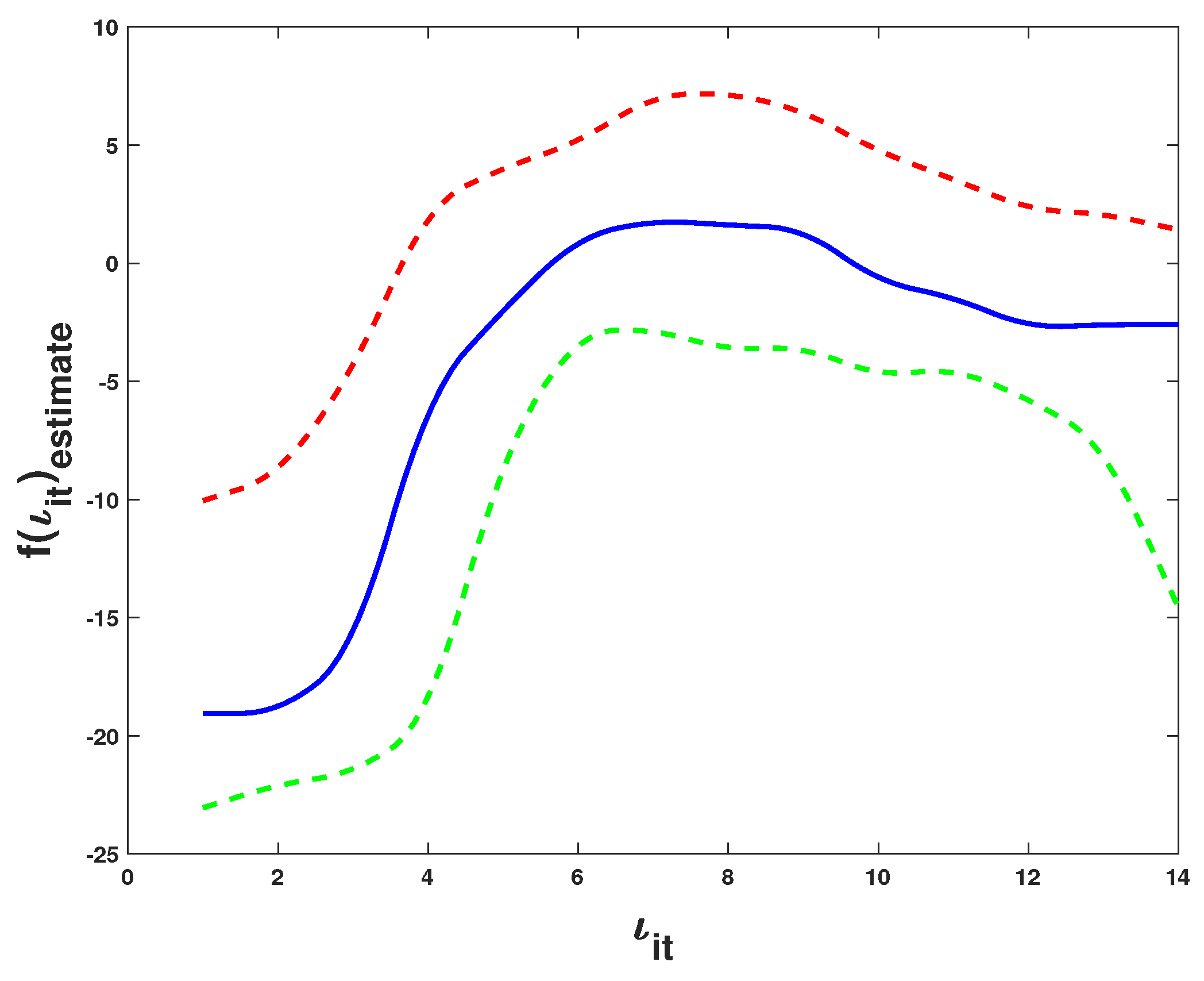
Table 11. Parameter estimation results.

Parameter	${\widehat{\mathit{\rho }}}_1$	${\widehat{\mathit{\rho }}}_2$	${\widehat{\mathit{\gamma }}}_1$	${\widehat{\mathit{\gamma }}}_2$	${\widehat{\mathit{\gamma }}}_3$	${\widehat{\mathit{\xi }}}_{\mathit{ϵ}}^2$	${\widehat{\mathit{\xi }}}_{\mathit{b}}^2$
Estimate	0.9018 ***	0.0124 ***	0.2818 ***	0.4881 ***	0.0020 ***	0.3140 ***	0.2907 ***

Note: *** presents that it is significant under test level 1%.

Figure 6 presents $\widehat{f}\left(\iota \right)$ and its 95% confidence interval, where the blue short dashed curve denotes $\widehat{f}\left(\iota \right)$, and the red and green solid curves correspond to the 95% confidence bands. Clearly, $landarea$ has a nonlinear effect on rice yield.

Figure 6. The nonlinear effect of ${\iota }_{it}$($landarea$) on $y_{it}$($log\left(rice\right)$).

6. Summary

This study mainly explores the PQMLE and F-test of RESPM with serially and spatially correlated nonseparable error. Our model simultaneously captures the linear and nonlinear effects of the covariates of spatially and serially correlated errors and individual random effects. PQMLEs are constructed for unknowns along with test statistic $F_{NT}$ to determine the beingness of nonlinear relationships. Their asymptotic properties are derived under regular conditions. The Monte Carlo results indicate that the proposed estimators and test statistic behave well on finite samples and that ignoring the spatial and serial correlations of errors may lead to inefficient and biased estimators. The proposed estimation and testing techniques are used to analyze Indonesian rice farming data.

The paper can be extended in several ways. We can apply spline estimation method or local polynomial method to approximate the nonparametric function, and combine GMM (Cheng and Chen [46]), quadratic inference function estimation (Qu [47]) or PQMLE to obtain the estimators of unknowns. Additionally, we can also consider extending these methods to other similar models, and the Bayesian analysis, variable selection, and quantile regression analysis of these models are also worth studying. In the future, we may use the proposed estimation and test methods to conduct empirical analysis, for example, investigating the drivers of $C{O}_2$, $P{M}_{2.5}$ and energy efficiency.

References

- Cheng, S.; Chen, J. GMM estimation of partially linear additive spatial autoregressive model. Comput. Stat. Data Anal. 2023, 182, 107712. [Google Scholar] [CrossRef]
- Chamberlain, G. Multivariate regression models for panel data. J. Econ. 1982, 18, 5–46. [Google Scholar] [CrossRef]
- Chamberlain, G. Panel data. Handb. Econom. 1984, 2, 1247–1318. [Google Scholar]
- Hsiao, C. Analysis of Panel Data; Cambridge University Press: Cambridge, UK, 2022; Volume 64. [Google Scholar]
- Baltagi, B.H. Econometric Analysis of Panel Data; Springer: Berlin/Heidelberg, Germany, 2008. [Google Scholar]
- Arellano, M. Panel Data Econometrics; Oxford University Press: Oxford, UK, 2003. [Google Scholar]
- Wooldridge, J.M. Econometric Analysis of Cross Section and Panel Data; MIT Press: Cambridge, MA, USA, 2010. [Google Scholar]
- Thapa, S.; Lomholt, M.A.; Krog, J.; Cherstvy, A.G.; Metzler, R. Bayesian analysis of single-particle tracking data using the nested-sampling algorithm: Maximum-likelihood model selection applied to stochastic-diffusivity data. Phys. Chem. Chem. Phys. 2018, 20, 29018–29037. [Google Scholar] [CrossRef] [PubMed]
- Rehfeldt, F.; Weiss, M. The random walker’s toolbox for analyzing single-particle tracking data. Soft Matter 2023, 19, 5206–5222. [Google Scholar] [CrossRef] [PubMed]
- Elhorst, J.P. Spatial Econometrics: From Cross-Sectional Data to Spatial Panels; Springer: Berlin/Heidelberg, Germany, 2014. [Google Scholar]
- Brueckner, J.K. Strategic interaction among governments: An overview of empirical studies. Int. Reg. Sci. Rev. 2003, 26, 175–188. [Google Scholar] [CrossRef]
- LeSage, J.P. An introduction to spatial econometrics. Rev. Econ. Ind. 2008, 123, 19–44. [Google Scholar]
- Elhorst, J.P. Applied spatial econometrics: Raising the bar. Spat. Econ. Anal. 2010, 5, 9–28. [Google Scholar] [CrossRef]
- Allers, M.; Elhorst, J. Tax mimicking and yardstick competition among local governments in The Netherlands. Int. Tax Public Financ. 2005, 12, 493–513. [Google Scholar] [CrossRef]
- Elhorst, J.P. Specification and estimation of spatial panel data models. Int. Reg. Sci. Rev. 2003, 26, 244–268. [Google Scholar] [CrossRef]
- Baltagi, B.H.; Li, D. Prediction in the panel data model with spatial correlation. In Advances in Spatial Econometrics: Methodology, Tools and Applications; Springer: Berlin/Heidelberg, Germany, 2004; pp. 283–295. [Google Scholar]
- Pesaran, M.H. General diagnostic tests for cross-sectional dependence in panels. Empir. Econ. 2021, 60, 13–50. [Google Scholar] [CrossRef]
- Kapoor, M.; Kelejian, H.H.; Prucha, I.R. Panel data models with spatially correlated error components. J. Econ. 2007, 140, 97–130. [Google Scholar] [CrossRef]
- Lee, L.; Yu, J. Estimation of spatial autoregressive panel data models with fixed effects. J. Econ. 2010, 154, 165–185. [Google Scholar] [CrossRef]
- Mutl, J.; Pfaffermayr, M. The Hausman test in a Cliff and Ord panel model. Econ. J. 2011, 14, 48–76. [Google Scholar] [CrossRef]
- Baltagi, B.H.; Egger, P.; Pfaffermayr, M. A generalized spatial panel data model with random effects. Econ. Rev. 2013, 32, 650–685. [Google Scholar] [CrossRef]
- Anselin, L. The Scope of Spatial Econometrics. In Spatial Econometrics: Methods and Models; Springer: Dordrecht, The Netherlands, 1988; pp. 7–15. [Google Scholar]
- Baltagi, B.H.; Song, S.H.; Koh, W. Testing panel data regression models with spatial error correlation. J. Econ. 2003, 117, 123–150. [Google Scholar] [CrossRef]
- Bordignon, M.; Cerniglia, F.; Revelli, F. In search of yardstick competition: A spatial analysis of Italian municipality property tax setting. J. Urban Econ. 2003, 54, 199–217. [Google Scholar] [CrossRef]
- Kelejian, H.H.; Prucha, I.R. On the asymptotic distribution of the Moran I test statistic with applications. J. Econ. 2001, 104, 219–257. [Google Scholar] [CrossRef]
- Cohen, J.P.; Paul, C.J. Public infrastructure investment, interstate spatial spillovers, and manufacturing costs. Rev. Econ. Stat. 2004, 86, 551–560. [Google Scholar] [CrossRef]
- Lee, L.; Yu, J. Spatial panels: Random components versus fixed effects. Int. Econ. Rev. 2012, 53, 1369–1412. [Google Scholar] [CrossRef]
- Parent, O.; LeSage, J.P. A space–time filter for panel data models containing random effects. Comput. Stat. Data Anal. 2011, 55, 475–490. [Google Scholar] [CrossRef]
- Elhorst, J.P. Serial and spatial error correlation. Econ. Lett. 2008, 100, 422–424. [Google Scholar] [CrossRef]
- Lee, L.; Yu, J. Estimation of fixed effects panel regression models with separable and nonseparable space–time filters. J. Econ. 2015, 184, 174–192. [Google Scholar] [CrossRef]
- Zhao, J.; Zhao, Y.; Lin, J.; Miao, Z.X.; Khaled, W. Estimation and testing for panel data partially linear single-index models with errors correlated in space and time. Random Matrices Theory Appl. 2020, 9, 2150005. [Google Scholar] [CrossRef]
- Li, S.; Chen, J.; Li, B. Estimation and Testing of Random Effects Semiparametric Regression Model with Separable Space-Time Filters. Fractal Fract. 2022, 6, 735. [Google Scholar] [CrossRef]
- Li, B.; Chen, J.; Li, S. Estimation of Fixed Effects Partially Linear Varying Coefficient Panel Data Regression Model with Nonseparable Space-Time Filters. Mathematics 2023, 11, 1531. [Google Scholar] [CrossRef]
- Bai, Y.; Hu, J.; You, J. Panel data partially linear varying-coefficient model with errors correlated in space and time. Stat. Sin. 2015, 35, 275–294. [Google Scholar]
- Cai, Z. Trending time-varying coefficient time series models with serially correlated errors. J. Econ. 2007, 136, 163–188. [Google Scholar] [CrossRef]
- Fan, J.; Zhang, C.; Zhang, J. Generalized likelihood ratio statistics and Wilks phenomenon. Ann. Stat. 2001, 29, 153–193. [Google Scholar] [CrossRef]
- Su, L.; Jin, S. Profile quasi-maximum likelihood estimation of partially linear spatial autoregressive models. J. Econ. 2010, 157, 18–33. [Google Scholar] [CrossRef]
- Lee, L. Asymptotic distributions of quasi-maximum likelihood estimators for spatial autoregressive models. Econometrica 2004, 72, 1899–1925. [Google Scholar] [CrossRef]
- Hamilton, S.A.; Truong, Y.K. Local linear estimation in partly linear models. J. Multivar. Anal. 1997, 60, 1–19. [Google Scholar] [CrossRef]
- Su, L.; Ullah, A. Nonparametric and semiparametric panel econometric models: Estimation and testing. In Handbook of Empirical Economics and Finance; CRC: Boca Raton, FL, USA, 2011; pp. 455–497. [Google Scholar]
- Su, L.; Ullah, A. Profile likelihood estimation of partially linear panel data models with fixed effects. Econ. Lett. 2006, 92, 75–81. [Google Scholar] [CrossRef]
- Su, L. Semiparametric GMM estimation of spatial autoregressive models. J. Econ. 2012, 167, 543–560. [Google Scholar] [CrossRef]
- Mack, Y.; Silverman, B.W. Weak and strong uniform consistency of kernel regression estimates. Z. Wahrscheinlichkeitstheorie Verwandte Geb. 1982, 61, 405–415. [Google Scholar] [CrossRef]
- Feng, Q.; Horrace, W.C. Alternative technical efficiency measures: Skew, bias, and scale. J. Appl. Econ. 2010, 27, 253–268. [Google Scholar] [CrossRef]
- Druska, V.; Horrace, W.C. Generalized moments estimation for spatial panel data: Indonesian rice farming. Am. J. Agric. Econ. 2004, 86, 185–198. [Google Scholar] [CrossRef]
- Cheng, S.; Chen, J. Estimation of partially linear single-index spatial autoregressive model. Stat. Pap. 2021, 62, 495–531. [Google Scholar] [CrossRef]
- Qu, A.; Lindsay, B.G.; Li, B. Improving generalized estimating equations using quadratic inference functions. Biometrika 2000, 87, 823–836. [Google Scholar] [CrossRef]
- White, H. Estimation, Inference and Specification Analysis; Cambridge University Press: Cambridge, UK, 1996. [Google Scholar]
Disclaimer/Publisher’s Note: The statements, opinions and data contained in all publications are solely those of the individual author(s) and contributor(s) and not of MDPI and/or the editor(s). MDPI and/or the editor(s) disclaim responsibility for any injury to people or property resulting from any ideas, methods, instructions or products referred to in the content. |
© 2024 by the authors. Licensee MDPI, Basel, Switzerland. This article is an open access article distributed under the terms and conditions of the Creative Commons Attribution (CC BY) license (https://creativecommons.org/licenses/by/4.0/).