New Perturbation–Iteration Algorithm for Nonlinear Heat Transfer of Fractional Order

Abstract

Ordinary differential equations have recently been extended to fractional equations that are transformed using fractional differential equations. These fractional equations are believed to have high accuracy and low computational cost compared to ordinary differential equations. For the first time, this paper focuses on extending the nonlinear heat equations to a fractional order in a Caputo order. A new perturbation iteration algorithm (PIA) of the fractional order is applied to solve the nonlinear heat equations. Solving numerical problems that involve fractional differential equations can be challenging due to their inherent complexity and high computational cost. To overcome these challenges, there is a need to develop numerical schemes such as the PIA method. This method can provide approximate solutions to problems that involve classical fractional derivatives. The results obtained from this algorithm are compared with those obtained from the perturbation iteration method (PIM), the variational iteration method (VIM), and the Bezier curve method (BCM). All solutions are tested with numerical simulations. The study found that the new PIA algorithm performs better than the PIM, VIM, and BCM, achieving high accuracy and low computational cost. One significant advantage of this algorithm is that the solutions obtained have established that the fractional values of alpha, specifically $\alpha$, significantly influencing the accuracy of the outcome and the associated computational cost.

1. Introduction

Many engineering problems that involve heat transfer equations are often nonlinear, making analytical solutions challenging. The perturbation method is an approach that solves these nonlinear problems by identifying small or large parameters known as the perturbation parameters [1,2]. This method has successfully solved ordinary differential equations [3], but only a few studies have explored its extension to fractional-order problems.

However, the concept of fractional calculus has its roots in the musings of Gottfried Wilhelm Leibniz from 1695, exploring the meaning of a derivative that was half ($\frac{1}{2}$) an order [4,5]. Since then, various pioneers such as Liouville, Grünwald, Letnikov, Riemman, and Caputo have developed a theory of derivatives and integrals of arbitrary order [6,7,8,9].

Over the last few decades, there has been a significant increase in the application of fractional calculus to real-world problems. Using dynamical systems described by fractional differential equations (FDEs) has become a way to understand complex materials and processes [10]. FDEs are capable of modeling non-locality, memory, spatial heterogeneity, and anomalous diffusion that are inherent in many real-world problems, making them useful in fields such as dynamical modeling [11], biology [12], chemistry [13], hydrology [14], control, signal and image processing, and finance [15].

FDEs assist in the computation of nonlinear complex systems by interpolating between integer orders of differential equations to capture non-local relations in time and space using power-law memory kernels [16]. The growing interest in FDEs has led to a global focus on finding new theoretical and numerical methods to solve fractional dynamical systems.

Various approaches can be taken when dealing with weak and nonlinear solid problems. One of these is iteration procedures, which involve the homotopy analysis method of nonlinear equations arising in heat transfer [17] and the iteration perturbation method [18]. The iteration procedure is carried out via an operational matrix [19]. The non-perturbative variational iteration method (VIM) was developed in [20].

In a research article in [21], an iterative finite difference (IFD) scheme was presented to simultaneously approximate both branches of a two-branched solution to the one-dimensional Bratu problem. Initially, the author introduced a transformation to convert Bratu’s problem into a simpler one. The transformed nonlinear ordinary differential equation was then discretized using the Newton–Raphson–Kantorovich approximation in function space. In another research article by Feng [22], accurate and real-time orbit computational methods are highly required for space tasks involving space vehicles. To solve relative orbit transfer problems efficiently and accurately, decoupling and quasi-linearization methods were proposed. The orbit transfer problem is transformed into a group of orbit propagation problems that are much easier to solve. Additionally, Ref. [23] developed a new variational iteration method using the quasilinearization method and Adomian polynomial to solve nonlinear differential equations. The article also discusses the convergence analysis of the new method under the Lipschitz continuity condition in Banach space.

Solving numerical problems that involve fractional differential equations can be challenging due to their inherent complexity and high computational cost. Heat equations, in particular, present significant difficulties because of the pseudodifferential and non-local nature of fractional operators. To overcome these challenges, there is a need to develop numerical schemes such as the perturbation–iteration algorithm (PIA) method. This method can provide approximate solutions to problems that involve classical fractional derivatives. This study is significant because it uses the PIA approach to improve the speed and accuracy of researchers’ work. The PIA method also reduces the time spent constructing algorithms.

To this end, this paper introduces the basic concept of the PIA and its application in solving a few heat transfer equations. Furthermore, it solves the nonlinear equations of the heat radiation. The solutions obtained by the PIA are compared with the previous works.

1.1. Research Questions

This article intends to answer the following questions:

• Can a PIA be constructed to solve heat transfer equation problems, considering their inherent complexity and high computational cost?
• Can the PIA provide approximate solutions to problems that involve heat transfer equations?
• Can a new PIA, believed to have high accuracy and low computational cost, compare to other methods?

The paper is structured as follows: Section 1.1 introduces the heat transfer equation. Section 2 presents the concept of the heat equations. Perturbation–iteration algorithms PIA(n,m) are presented in Section 3, along with the convergence analysis of PIA(1,1) and PIA(1,2) in Section 3.1 and Section 3.2, respectively. The applications of the PIA to heat transfer problems are presented in Section 4. We provide a discussion in Section 5 and conclude the paper in Section 6.

Let define the fractional-order definition to use here for $\alpha$-th, which is of the order $D_t^{\alpha }u$ of $f\left(t\right)$. The following properties can be found in the works of [1,24]. These definitions and results play a critical role in understanding the fundamental concepts and principles of fractional calculus and are integral to completing this paper’s endeavor. Therefore, it is essential to comprehend these concepts before proceeding with the paper.

Definition 1.

The Riemann–Liouville integral with order $\alpha >0$ of given function $f\left(t\right)$ is defined as:

$${}_x{}^{y}D^{\varphi }f\left(u\right)={\int }_x^y\varpi \left(\varphi \right)\left[D^{\varphi }f\left(u\right)\right]dv={\int }_x^y\left[\frac{\varpi \left(\varphi \right)}{\Gamma (1-\varphi )}\right]{\int }_x^y{(\varphi -t)}^{-\varphi }{f}^{\prime }\left(t\right)dt,$$

(1)

where $\varpi \left(\varphi \right)$ represent the weight function.

Caputo put forth a modification to the Riemann–Liouville fractional derivative, suggesting that the convolution integral be factored in prior to the $n-$ derivative instead of afterwards, as had been the norm. In contrast to the Riemann–Liouville fractional derivative, Caputo’s method does not require fractional-order initial conditions to be defined when resolving differential equations. The equation below depicts Caputo’s definition, where $n=⌈\alpha ⌉$ [9,25].

$${}^{C}D^{\alpha }f\left(t\right)=\frac{1}{\Gamma (n-\alpha )}{\int }_0^t{(t-x)}^{n-\alpha -1}\frac{d^n}{d{x}^n}f\left(x\right)dx,\alpha >0,n=\lceil \alpha \rceil .$$

(2)

where $\Gamma$ and $\alpha$ are represented as the function of the Gamma and positive alpha, respectively. Take $f\left(t\right)$ as the solution to the initial value problem. When solving differential equations using Caputo’s approach, defining fractional-order beginning conditions is unnecessary, unlike Riemann–Liouville’s fractional derivative.

2. Concept of Heat Equations

This section will examine how a lumped system cools down by considering both convective and radiative heat transfer. The system has various characteristics, such as volume (V), surface area (A), density ($\eta$), specific heat ($\Phi$), and emissivity (E). In the beginning, the system’s temperature is $U_i$, and when $u=0$, it is exposed to an environment with a temperature of $U_a$ and a convective heat transfer coefficient of $\delta$. Additionally, the system loses heat through radiation, with an effective sink temperature of $U_s$. The cooling equation and initial conditions are as follows [20]:

$$\begin{array}{c}\hfill \eta V\Phi \frac{dU}{dt}+\delta A(U-U_a)+E\gamma A(U^4-u_s^4)=0,\\ \hfill u=0,U=U_i.\end{array}$$

(3)

To find the solution of Equation (3), we need to perform specific modifications to the parameters.

$$\tau =\frac{U}{U_i},{\tau }_a=\frac{U_a}{U_i},{\tau }_s={\frac{U_s}{U_i}}^{\prime }\kappa =\frac{u}{\frac{\eta V{\Phi }_a}{\delta A}}.$$

(4)

After changing the parameters, the heat transfer equation will be modified and result in the following outcome:

$$\begin{array}{c}\hfill \frac{d\theta }{d\kappa }+(\theta -{\theta }_a)-ϵ({\theta }^4-{\theta }_a^4)=0,\\ \hfill \kappa =0,\theta =1.\end{array}$$

(5)

To simplify Equation (5), we assume the case where $a=s=0$ and consider the fractional order in the sense of Caputo. Thus, under these assumptions, we can express Equation (5) in a simplified form. The Caputo derivative is a modification of the Riemann–Liouville derivative that allows for the fractional derivative of a function to be defined at its initial value. By simplifying the equation in the fractional order, we can better understand how it behaves and make more accurate predictions based on its properties:

$${}_0{}^{c}D_t^{\theta }u\left(t\right)+u+ϵu^4=0,0<\theta \le 1,0<t<1,$$

(6)

with conditions $\kappa =0,\theta =1$, where $ϵ$ is the dimensionless radiation parameter.

3. PIA(n,m) Perturbation–Iteration Algorithms

This section introduces a systematic approach that enables the quick construction of new algorithms using PIA(n,m)—where ’n’ represents the number of correction terms in the perturbation expansion and ’m’ denotes the order of derivatives in the Taylor series expansions, with $n\le m)$. This methodology provides a convenient technique to generate algorithms with the abovementioned parameters, helping researchers enhance their work’s accuracy and speed while minimizing the time spent constructing algorithms.

3.1. PIA(1,1) Convergence Analysis

This section will introduce the PIA(1,1) algorithm, a perturbation–iteration method that uses a single correction term in the perturbation expansion. Additionally, correction terms will be used for the first derivatives in the Taylor series expansion. The algorithm employs $n=1$ and $m=1$. Our focus will be on analyzing a second-order differential equation.

$$F(u^{″},u,ϵ)=0$$

(7)

When considering Equation (7) with a time-dependent variable $u\left(t\right)$ and a perturbation parameter $ϵ$, it is possible to incorporate a correction term for perturbation expansion. This expansion requires only one correction term, which can be expressed concisely.

$$u_{n+1}=u_n+ϵ{\left(u_c\right)}_n.$$

(8)

To obtain the necessary solution, we can substitute Equation (8) into Equation (7) and expand it utilizing a Taylor series with only first derivatives.

$$F(u_n^{″},u_n,0)+F_u(u_n^{″},u_n,0)ϵ{\left(u_c\right)}_n+F_{u^{″}}(u_{″},u_{n,0})ϵ{\left(u_c\right)}_n+F_{ϵ}(u_n^{″},u_n,0)ϵ=0.$$

(9)

When differentiating with respect to the independent variable, let ${\left(\right)}^{\prime }$ represent the operation. Furthermore, let

$$F_{ϵ}=\frac{\partial F}{\partial ϵ},F_u=\frac{\partial F}{\partial u},F_{u^{\prime }}=\frac{\partial F}{\partial u^{\prime }},\dots$$

(10)

The equation can be reorganized as follows:

$${\left(u_n^{″}\right)}_n+\frac{F_u}{F_u^{″}}{\left(u_c\right)}_n=-\frac{F_{ϵ}+\frac{F}{ϵ}}{F_u^{″}}$$

(11)

It is important to note that all derivatives in the equation are evaluated at $ϵ=0$, implying that it is a variable-coefficient, linear, second-order differential equation. Therefore, to solve this equation, we need to begin with an initial guess $u_0$ and then calculate ${\left(u_c\right)}_n$ using Equation (11). Subsequently, we should substitute ${\left(u_c\right)}_0$ into Equation (8) to calculate $u_1$. The iteration procedure, using Equations (11) and (8), should be repeated until we obtain a satisfactory result. It is worth mentioning that this iteration algorithm may produce similar results to the variational iteration algorithm II, which is explained in [26]. Further details about the proposed three different variational iteration algorithms can be found in [26].

3.2. PIA(1,2) Convergence Analysis

The present subsection presents an efficient perturbation–iteration algorithm to obtain the correction terms in the perturbation and Taylor series expansions. By considering correction terms up to second derivatives in the Taylor series expansion and one correction term in the perturbation expansion, the resulting algorithm, named PIA(1, 2), is confidently developed. The correction term in Equation (8) is incorporated into (7), which is developed into a Taylor series up to second-order derivatives. After rearrangement, the algorithm yields the following result.

$$\begin{array}{cc}\hfill F(u_n^{″},u_n,0)& +F_u^{″}(u_n^{″},u_n,0)ϵ{\left(u_c\right)}_n+F_u(u_n^{″},u_n,0)ϵ{\left(u_c\right)}_n+F_u^{″}(u_n^{″},u_n,0)ϵ{\left(u_c\right)}_n\hfill \\ \hfill & +\frac{1}{2}{F}_{ϵϵ}(u_n^{″},u_n,0){ϵ}^2+\frac{1}{2}{F}_{u^{″}{u}^{″}}(u_n^{″},u_n,0){ϵ}^2{\left(u_n^{″}\right)}_n^2+\frac{1}{2}{F}_{uu}(u_n^{″},u_n,0){ϵ}^2{\left(u_n^{″}\right)}_n^2\hfill \\ \hfill & +F_{u^{″}u}(u_n^{″},u_n,0){ϵ}^2{\left(u_c^{″}\right)}_n{u_c}_n+F_{u^{\prime \prime }ϵ}(u_n^{″},u_n,0){ϵ}^2{\left(u_c^{″}\right)}_n+F_{uϵ}(u_n^{″},u_n,0){ϵ}^2{\left(u_c^{″}\right)}_n.\hfill \end{array}$$

(12)

Equation (12) becomes

$$\begin{array}{cc}\hfill (ϵF_u^{″}& +{ϵ}^2{F}_u^{″}ϵ){\left(u_c^{″}\right)}_n+(ϵF_u+{ϵ}^2{F}_uϵ){\left(u_c\right)}_n+\frac{1}{2}{F}_{u^{″}{u}^{″}}{\left(u_c^{″}\right)}_n^2+F_{u^{\prime \prime }u}{ϵ}^2{\left(u_c^{\prime \prime }\right)}_n{\left(u_c\right)}_n+\frac{1}{2}{F}_{uu}{\left(u_c^{″}\right)}_n^2\hfill \\ \hfill & =-F-F_{ϵ}ϵ-\frac{1}{2}{F}_{ϵϵ}{ϵ}^2\hfill \end{array}$$

(13)

As previously mentioned, when $ϵ=0$, all functions and their derivatives are evaluated. The equation provided is a second-order nonlinear differential equation with variable coefficients. To tackle this equation, we can utilize an iterative scheme constructed with Equations (8) and (13).

4. Applications of PIA to Heat Transfer Problems

We subjected the new PIA to a series of nonlinear heat transfer problems to evaluate its reliability. In order to demonstrate this, we need to utilize various examples, including cooling a lumped system through convection and radiation, distributing temperature in a uniformly thick rectangular fin through radiation to free space, and one-dimensional conduction in a slab with temperature-dependent thermal conductivity.

Example 1.

We first consider the fractional dimensionless nonlinear differential equation describing combined convection and radiation cooling of a lumped system [3]: as follows:

$${}_0{}^{c}D_t^{\theta }u\left(t\right)+u+ϵu^4=0,0<\theta \le 1,0<t<1,$$

(14)

with initial conditions $u\left(0\right)=1$, where ϵ is the dimensionless radiation parameter.

Solution: In order to solve problem (14), we use the robust fractional perturbation–iteration algorithm (PIA) and the iteration Formula (12). To start, we need a base function that is suitable for the boundary condition. Then, at each step, we calculate coefficients from the boundary condition using the iteration formula.

Before applying the PIA algorithm, we need to carefully evaluate the terms in the PIA formula. This will ensure that our calculations are based on a solid foundation. Once we have achieved this, we can confidently choose $ϵ$ value as the perturbation parameter. This simplifies the equation and makes it more manageable, allowing us to calculate the solution efficiently. This step is crucial for a successful application of the PIA algorithm. With this approach, we are confident that we can obtain the solution to (14) with a high degree of accuracy.

We can confirm that Equation (14) is valid in the Caputo fractional calculus framework by rephrasing it into the Caputo integral Equation (14). This confirms that the equation is correct within the Caputo fractional calculus framework.

$$\begin{array}{c}\hfill u^{\prime }\left(t\right)=-\frac{1}{\Gamma (1-\theta )}{\int }_0^x\frac{u_n^{\prime }\left(t\right)}{{(s-t)}^{\theta }}dt-u_n^4\left(t\right)-u_n^{\prime }\left(t\right)-u_n\left(t\right)\end{array}$$

(15)

Taking into consideration that $ϵ=1$, the following sequential approximate solutions are obtained at each stage using the iteration formula.

In Equation (12), F represents the terms in the iteration formula, with $F=u_{n^{\prime }}+u_n$, $F_{u^{\prime }}=0$, $F_u=1$, and $F_{ϵ}=-u_n^4$. Here, $ϵ$ is a small parameter introduced artificially. By setting $ϵ=0$, Equation (12) is reduced to

$${\left(u_c^{″}\right)}_n=-\frac{u_n^{\prime }+u_n}{ϵ}-u_n^4$$

(16)

To find the approximate solutions at each step, one can take a trivial solution that satisfies the initial conditions. It should be noted that the initial function is chosen to satisfy the boundary condition exactly. The equation is then approximated. As the number of iterations increases, it is worth noting that the complexity of the analytical solution also increases proportionally. Consequently, it becomes necessary to employ symbolic manipulation programs to handle the computations involved effectively.

$$u_0=e^{-t}$$

(17)

The approximate solutions can be determined using Equations (8) and (16).

$$\begin{array}{cc}\hfill u_1\left(t\right)& =e^{-t}-\frac{3}{16}{e}^{-4t}-\frac{1}{7}{e}^{-7t}+\frac{1}{80}{e}^{-10t}-\frac{1}{208}{e}^{-13t}+\frac{1}{4096}{e}^{-16t}\hfill \\ \hfill u_2\left(t\right)& =e^{-t}-\frac{13}{64}{e}^{-4t}-\frac{25}{196}{e}^{-7t}+\frac{1447}{44800}{e}^{-10t}-\frac{205123}{6056960}{e}^{-13t}+\frac{8337711}{3339714560}{e}^{-16t}\hfill \\ \hfill & -\frac{257077}{61967360}{e}^{-19t}+\frac{27271087}{20090470400}{e}^{-22t}+\frac{14706801}{730562560000}{e}^{-25t}-\frac{131763331643}{1191342977843200}{e}^{-28t}\hfill \\ \hfill & +\frac{1759374159}{58883342336000}{e}^{-31t}-\frac{4629610649}{2066615369728000}{e}^{-34t}-\frac{14923562267}{17991710277632000}{e}^{-37t}\hfill \\ \hfill & +\frac{1961031032599}{5779576428953600000}{e}^{-40t}-\frac{672983823}{9707882283008000}{e}^{-43t}+\frac{6459639521}{664651289329664000}{e}^{-46t}\hfill \\ \hfill & -\frac{325494581}{323656280021401600}{e}^{-49t}+\frac{5573683747}{71442169892071014400}{e}^{-52t}-\frac{324697}{72657532249702400}{e}^{-55t}\hfill \\ \hfill & +\frac{2427}{13471766219325440}{e}^{-58t}-\frac{1}{217978180206592}{e}^{-61t}+\frac{1}{18014398509481984}{e}^{-64t}.\hfill \end{array}$$

(18)

Example 2.

Secondly, we consider another value for (14) given as follows:

$${}_0{}^{c}D_t^{2\theta }u\left(t\right)-2e^{ϵu\left(t\right)}=0,0<\theta \le 1,0<t<1,$$

(19)

with initial condition $u\left(0\right)=u^{\left(\theta \right)}\left(0\right)=0$. The exact solution is known.

$$u\left(t\right)=-2\ln \left(\cos \right(t\left)\right)$$

(20)

Following the approach in Example 1 above, we can confirm Equation (20) as a valid expression in the Caputo fractional calculus framework by rephrasing it into the Caputo integral Equation (20). This ensures that the equation is correct within the Caputo fractional calculus framework, giving us

$$\begin{array}{c}\hfill u^{″}\left(t\right)=-\frac{1}{\Gamma (1-\theta )}{\int }_0^x\frac{u_n^{″}\left(t\right)}{{(s-t)}^{\theta }}dt+2u_n\left(t\right)+u_n^{″}\left(t\right)+2\end{array}$$

(21)

We evaluate the terms in (13) and then simplify the equation to

$${\left(u_c^{″}\right)}_n-{\left(u_c^{″}\right)}_n=u_n+u_n^2=(u_n^{″}-1)$$

(22)

by selecting $ϵ=1$ as shown in (28). Our initial assumption is

$$u_0=0,$$

(23)

which we substitute into (28) to obtain

$${\left(u_c^{″}\right)}_0=1+{\left(u_c\right)}_0.$$

(24)

Once we solve (24), we substitute the result into (8) and apply the initial conditions to derive the final solution.

$$\begin{array}{cc}\hfill u_1\left(t\right)& =t^2+\frac{1}{6}{t}^4\hfill \\ \hfill u_2\left(t\right)& =t^2+\frac{1}{6}{t}^4+\frac{1}{90}{t}^6+\frac{1}{2520}{t}^8\hfill \\ \hfill u_3\left(t\right)& =t^2+\frac{1}{6}{t}^4+\frac{1}{90}{t}^6+\frac{1}{2520}{t}^8+\frac{1}{113400}{t}^{10}+\frac{1}{7484400}{t}^{12}\hfill \\ \hfill u_4\left(t\right)& =t^2+\frac{1}{6}{t}^4+\frac{1}{90}{t}^6+\frac{1}{2520}{t}^8+\frac{1}{113400}{t}^{10}+\frac{1}{7484400}{t}^{12}\hfill \\ \hfill & +\frac{1}{681080400}{t}^{14}+\frac{1}{81729648000}{t}^{16}\hfill \\ \hfill u_5\left(t\right)& =t^2+\frac{1}{6}{t}^4+\frac{1}{90}{t}^6+\frac{1}{2520}{t}^8+\frac{1}{113400}{t}^{10}+\frac{1}{7484400}{t}^{12}\hfill \\ \hfill & +\frac{1}{681080400}{t}^{14}+\frac{1}{81729648000}{t}^{16}\hfill \\ \hfill & +\frac{1}{12504636144000}{t}^{18}+\frac{1}{2375880867360000}{t}^{20}.\hfill \end{array}$$

(25)

Example 3.

Thirdly, we consider the dimensionless nonlinear boundary value problem describing temperature distribution in a uniformly thick rectangular fin with radiation to free space [3], as follows:

$${}_0{}^{c}D_t^{\theta }u\left(t\right)-ϵu^4=0,0<\theta \le 1,0<t<1,$$

(26)

with initial condition $u^{\prime }\left(0\right)=0,u\left(1\right)=1$, where ϵ is our dimensionless radiation parameter. Second iteration analytical solutions are given by both methods.

Following the approach in Example 1 above, we can confirm Equation (26) as a valid expression in the Caputo fractional calculus framework by rephrasing it into the Caputo integral Equation (26). This ensures that the equation is correct within the Caputo fractional calculus framework, giving us

$$\begin{array}{c}\hfill u^{″}\left(t\right)=-\frac{1}{\Gamma (1-\theta )}{\int }_0^x\frac{u_n^{″}\left(t\right)}{{(s-t)}^{\theta }}dt+u_n^4\left(t\right)+u_n^{″}\left(t\right)\end{array}$$

(27)

We evaluate the terms in (13) and then simplify the equation to

$${\left(u_c^{″}\right)}_n-{\left(u_c^{″}\right)}_n=\frac{-u_n}{ϵ}+u_n^4$$

(28)

by selecting $ϵ=1$ as shown in (28). Our initial assumption is

$$u_0=1,$$

(29)

which we substitute into (28) to obtain

$${\left(u_c^{″}\right)}_0=+u_n^4\left(t\right)+u_n^{″}\left(t\right).$$

(30)

Once we solve (24), we substitute the result into (8) and apply the initial conditions to derive the final solution.

$$\begin{array}{cc}\hfill u_1\left(t\right)& =\frac{1}{2}t+\frac{1}{2}{t}^2\hfill \\ \hfill u_2\left(t\right)& =\frac{12193}{6720}t-\frac{1}{2}{t}^2-\frac{1}{3}{t}^3+\frac{1}{480}{t}^6\hfill \\ \hfill & +\frac{1}{168}{t}^7+\frac{3}{448}{t}^8+\frac{1}{288}{t}^9+\frac{1}{1440}{t}^2.\hfill \end{array}$$

(31)

5. Discussion

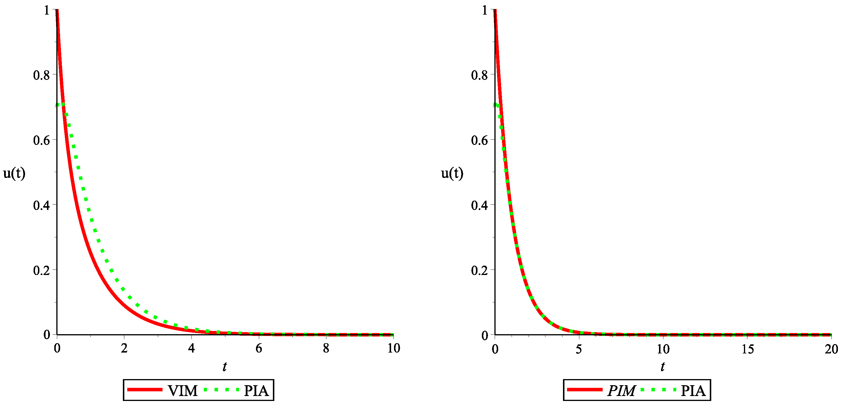
For Example 1, the results of the PIA, perturbation–iteration method (PIM), and variational iteration method (VIM) analyses were compared with the numerical solution in Figure 1 and Figure 2 and

Table 1. The comparison between the variational iteration method (VIM) and our solution when $\alpha =1,u_1\left(t\right)$ for Example 1.

t	VIM Solution $\mathit{u}\left(\mathit{t}\right)$	Our Solution $\mathit{u}\left(\mathit{t}\right)$	Absolute Error
0.0	1.0000000000	0.7025793054	2.97421 $\times {10}^{-1}$
0.1	0.9048374180	0.7207461728	1.84091 $\times {10}^{-1}$
0.2	0.8187307531	0.7039813749	1.14749 $\times {10}^{-1}$
0.3	0.7408182207	0.6686222379	7.21960 $\times {10}^{-2}$
0.4	0.6703200460	0.6244380174	4.58820 $\times {10}^{-2}$
0.5	0.6065306597	0.5770869090	2.94438 $\times {10}^{-2}$
0.6	0.5488116361	0.5297507944	1.90608 $\times {10}^{-2}$
0.7	0.4965853038	0.4841532815	1.24320 $\times {10}^{-2}$
0.8	0.4493289641	0.4411702189	8.15875 $\times {10}^{-3}$
1.9	0.4065696597	0.4011887205	5.38094 $\times {10}^{-3}$
1.0	0.3678794412	0.3643166816	3.56276 $\times {10}^{-3}$

and

Table 2. The comparison between the perturbation–iteration method (PIM) and our solution when $\alpha =1,u_1\left(t\right)$ for Example 1.

t	PIM Solution $\mathit{u}\left(\mathit{t}\right)$	Our Solution $\mathit{u}\left(\mathit{t}\right)$	Absolute Error
0.0	1.0000000000	0.7025793054	2.97421 $\times {10}^{-1}$
0.1	0.9048374180	0.7207461728	1.84091 $\times {10}^{-1}$
0.2	0.8187307531	0.7039813749	1.14749 $\times {10}^{-1}$
0.3	0.7408182207	0.6686222379	7.21960 $\times {10}^{-2}$
0.4	0.6703200460	0.6244380174	4.58820 $\times {10}^{-2}$
0.5	0.6065306597	0.5770869090	2.94438 $\times {10}^{-2}$
0.6	0.5488116361	0.5297507944	1.90608 $\times {10}^{-2}$
0.7	0.4965853038	0.4841532815	1.24320 $\times {10}^{-2}$
0.8	0.4493289641	0.4411702189	8.15875 $\times {10}^{-3}$
1.9	0.4065696597	0.4011887205	5.38094 $\times {10}^{-3}$
1.0	0.3678794412	0.3643166816	3.56276 $\times {10}^{-3}$

. All methods used the same initial trial function and number of iterations. It was discovered that our proposed solution provided better agreement with the numerical solution. Figure 2 compares all three perturbation–iteration solutions with the numerical ones. The accuracy of the solutions improved as the number of iterations increased. The absolute errors are in Table 1 and Table 2. The figure shows that the absolute error of the PIA with only one iteration was better than that of PIM and VIM with two iterations.

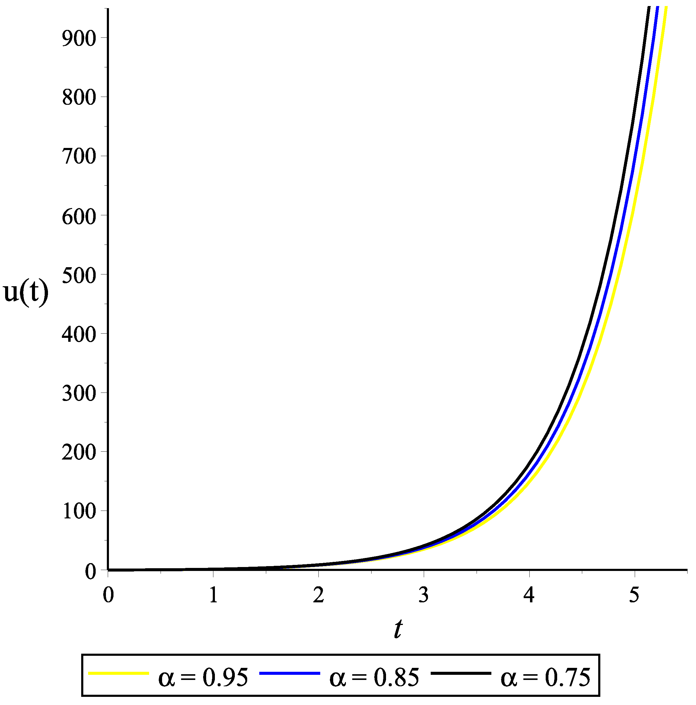
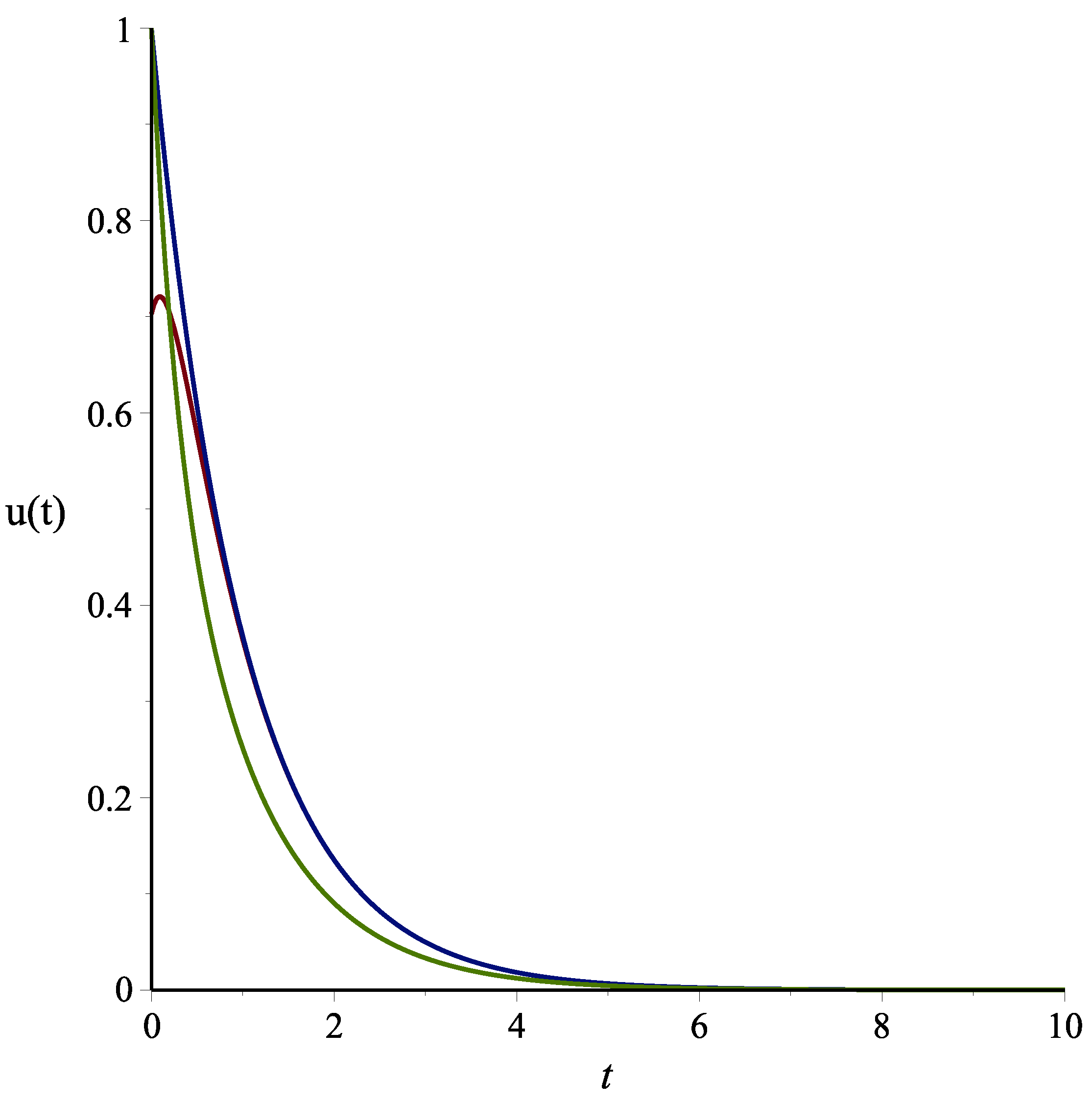
The approach suggested is demonstrated to be effective and accurate in Figure 3, where the results are compared with the exact solutions.

Table 3. Comparison between exact and our solutions of Example 2.

n	Our Solution	Exact Solution	Error
0.1	0.0100166778	0.0100167112	3.34200 $\times {10}^{-8}$
0.2	0.0402673788	0.0402695462	2.16738 $\times {10}^{-6}$
0.3	0.0913581261	0.0913833119	2.51858 $\times {10}^{-5}$
0.4	0.1643124388	0.1644580382	1.45599 $\times {10}^{-4}$
0.5	0.2605918365	0.2611684808	5.76644 $\times {10}^{-4}$
0.6	0.3821251187	0.3839303388	1.80522 $\times {10}^{-3}$
0.7	0.5313470049	0.5361715150	4.82451 $\times {10}^{-3}$
0.8	0.7112469103	0.7227814938	1.15346 $\times {10}^{-2}$
0.9	0.9254288331	0.9508848870	2.54561 $\times {10}^{-2}$
1.0	1.1781835560	1.2312529410	5.30694 $\times {10}^{-2}$

and

Table 4. The comparison between our method with the Bezier curve method (BCM) in [27] when $\alpha =1.9$ for Example 2.

n	Our Solution	BCM Solution	Error
0.1	0.0060821388	0.01031561203	3.93457 $\times {10}^{-3}$
0.2	0.0245519985	0.04026954618	1.57175 $\times {10}^{-2}$
0.3	0.0560975280	0.09121393595	3.52858 $\times {10}^{-2}$
0.4	0.1012032928	0.1643473163	6.32547 $\times {10}^{-2}$
0.5	0.1599660154	0.2611684808	1.01202 $\times {10}^{-1}$
0.6	0.2320244206	0.3839303388	1.51906 $\times {10}^{-1}$
0.7	0.3165466912	0.3839303388	2.19625 $\times {10}^{-1}$
0.8	0.4122688303	0.7227814938	3.10513 $\times {10}^{-1}$
0.9	0.5175820617	0.9512319022	4.33303 $\times {10}^{-1}$
1.0	0.6306676970	1.231252941	6.00585 $\times {10}^{-1}$

supports this assertion. Furthermore, Figure 4 displays the reaction of $\alpha$ with different values, namely $\alpha =0.95,0.85,0.5$ for Example 2.

Table 5. Comparison between the solutions of the perturbation–iteration method (PIM) and our method for Example 3 when $ϵ=1$, and $u_1\left(t\right)$.

t	PIM Solution	Our Solution	Absolute Error
0.0	0.6666666667	0.0000000000	6.66667 $\times {10}^{-1}$
0.1	0.6700000000	0.0550000000	6.15000 $\times {10}^{-1}$
0.2	0.6800000000	0.1200000000	5.60000 $\times {10}^{-1}$
0.3	0.6966666667	0.1950000000	5.01667 $\times {10}^{-1}$
0.4	0.7200000000	0.2800000000	4.40000 $\times {10}^{-1}$
0.5	0.7500000000	0.3750000000	3.75000 $\times {10}^{-1}$
0.6	0.7866666667	0.4800000000	3.06667 $\times {10}^{-1}$
0.7	0.8300000000	0.5950000000	2.35000 $\times {10}^{-1}$
0.8	0.8800000000	0.7200000000	1.60000 $\times {10}^{-1}$
0.9	0.9366666667	0.8550000000	8.16667 $\times {10}^{-2}$

and

Table 6. The comparison between our solution and the variational iteration method (VIM) in [3] when $\alpha =1$ for Example 3 for $ϵ=1$, and $u_1\left(t\right)$.

t	VIM Solution	Our Solution	Absolute Error
0.0	0.8164505572	0.0000000000	8.16451 $\times {10}^{-1}$
0.1	0.8177840043	0.0550000000	7.62784 $\times {10}^{-1}$
0.2	0.8218378615	0.1200000000	7.01838 $\times {10}^{-1}$
0.3	0.8287748243	0.1950000000	6.33775 $\times {10}^{-1}$
0.4	0.8388732974	0.2800000000	5.58873 $\times {10}^{-1}$
0.5	0.8525385680	0.3750000000	4.77539 $\times {10}^{-1}$
0.6	0.8703190713	0.4800000000	3.90319 $\times {10}^{-1}$
0.7	0.8929284015	0.5950000000	2.97928 $\times {10}^{-1}$
0.8	0.9212739503	0.7200000000	2.01274 $\times {10}^{-1}$
0.9	0.9564933240	0.8550000000	1.01493 $\times {10}^{-1}$

compare two analytical methods, the perturbation–iteration method (PIM) and variational iteration method (VIM), with our proposed fractional PIA. The PIA exhibits remarkable accuracy when compared to numerical solutions. Lastly, a comparison of results for our solution, the PIA, when $\alpha =1.00,0.95,0.85,0.75$ for Example 3 is presented in

Table 7. The comparison of results for our solution, the PIA, when $\alpha =1.00,0.95,0.85,0.75$ for Example 3.

t	$\mathit{\alpha }=1.00$	$\mathit{\alpha }=0.95$	$\mathit{\alpha }=0.85$	$\mathit{\alpha }=0.75$
0.1	0.17611	0.17435	0.17091	0.16762
0.2	0.34022	0.33727	0.33142	0.32570
0.3	0.49033	0.48666	0.47925	0.47191
0.4	0.62446	0.62046	0.61230	0.60410
0.5	0.74066	0.73669	0.72850	0.72016
0.6	0.83708	0.83344	0.82588	0.81809
0.7	0.91205	0.90903	0.90269	0.89606
0.8	0.96434	0.96216	0.95753	0.95265
0.9	0.99342	0.99226	0.98977	0.98712
1.0	1.00000	1.00000	0.99999	1.00000

. The findings above have established that the fractional values of $\alpha$ significantly influence the accuracy of the outcome and the associated computational cost.

6. Conclusions

We conclude that all our three research questions were duly answered and addressed. The PIA was constructed to solve heat transfer equation problems due to their inherent complexity and high computational cost. The PIA was able to provide approximate solutions to problems that involve heat transfer, and the new PIA is shown to have high accuracy and low computational cost compare to other methods. We used the PIA to construct and compare them with numerical solutions. Our approach converted the nonlinear differential equation into a nonlinear algebraic fractional system. We analyzed various forms of the fractional heat equation with different parameters and fractional derivative orders in the Caputo sense. Our introduced method is proven to be convergent. We present the results obtained in tables and graphs for comparison. These results demonstrate the accuracy and convergence of the solutions. Since the heat equation is nonlinear, the method used in approximating the solutions has acceptable accuracy and performance.

However, the proposed new operational matrix method should be extended to solve some other tempered fractional calculus problems, such as tempered fractional partial differential equations.

We have successfully answered all three of our research questions regarding the construction and implementation of the PIA method for solving complex heat transfer equation problems. The PIA method is particularly useful due to the high computational cost and complexity of these problems. By providing approximate solutions, the PIA has proven to be a highly accurate and cost-effective alternative to other methods. We utilized the PIA method to compare and construct numerical solutions, converting nonlinear differential equations into nonlinear algebraic fractional systems. We analyzed various forms of the fractional heat equation with different parameters and fractional derivative orders in the Caputo sense and have proven our approach to be convergent. Our results, presented in tables and graphs, demonstrate the accuracy and convergence of the solutions.

However, it is suggested that the proposed PIA method should be further developed to solve other related problems in fractional calculus, including tempered fractional partial differential equations.

References

1. Şenol, M.; Dolapci, I.T. On the perturbation–iteration algorithm for fractional differential equations. J. King Saud Univ. Sci. 2016, 28, 69–74. [Google Scholar] [CrossRef]
2. Pakdemirli, M. Review of the new perturbation-iteration method. Math. Comput. Appl. 2013, 18, 139–151. [Google Scholar] [CrossRef]
3. Aksoy, Y.; Pakdemirli, M.; Abbasbandy, S.; Boyacı, H. New perturbation-iteration solutions for nonlinear heat transfer equations. Int. J. Numer. Methods Heat Fluid Flow 2012, 22, 814–828. [Google Scholar] [CrossRef]
4. Cajori, F. The history of notations of the calculus. Ann. Math. 1923, 25, 1–46. [Google Scholar] [CrossRef]
5. Leibniz, G.W.; Heer, F. Gottfried Wilhelm Leibniz; Fischer Bücherei: Gütersloh, Germany, 1958. [Google Scholar]
6. Morita, T.; Sato, K.-i. Liouville and riemann-liouville fractional derivatives via contour integrals. Fract. Calc. Appl. Anal. 2013, 16, 630–653. [Google Scholar] [CrossRef]
7. Malinowska, A.B.; Odzijewicz, T.; Torres, D.F. Advanced Methods in the Fractional Calculus of Variations; Springer: Berlin/Heidelberg, Germany, 2015. [Google Scholar]
8. Oliveira, D.S.; de Oliveira, E.C. On a caputo-type fractional derivative. Adv. Pure Appl. Math. 2019, 10, 81–91. [Google Scholar] [CrossRef]
9. Abdeljawad, T. On riemann and caputo fractional differences. Comput. Math. Appl. 2011, 62, 1602–1611. [Google Scholar] [CrossRef]
10. Owoyemi, A.E.; Sulaiman, I.M.; Mamat, M.; Olowo, S.E.; Adebiyi, O.A.; Zakaria, Z.A. Analytic numeric solution of coronavirus (COVID-19) pandemic model in fractional-order. Commun. Math. Biol. Neurosci. 2020, 2020. [Google Scholar]
11. Owoyemi, A.E.; Sulaiman, I.M.; Kumar, P.; Govindaraj, V.; Mamat, M. Some novel mathematical analysis on the fractional-order 2019-ncov dynamical model. Math. Methods Appl. Sci. 2023, 46, 4466–4474. [Google Scholar] [CrossRef]
12. Owoyemi, A.E.; Sulaiman, I.M.; Mamat, M.; Olowo, S.E. Stability and bifurcation analysis in a fractional-order epidemic model with sub-optimal immunity, nonlinear incidence and saturated recovery rate. Iaeng Int. J. Appl. Math. 2021, 51. [Google Scholar]
13. Phaochoo, P.; Wisseksakwichai, C.; Thongpool, N.; Chankong, S.; Promluang, K. Application of fractional derivative for the study of chemical reaction. Int. J. Intell. Netw. 2023, 13, 2245. [Google Scholar]
14. Xiang, X.; Ao, T.; Li, X. Application of a fractional instantaneous unit hydrograph in the topmodel: A case study in chengcun basin, China. Appl. Sci. 2023, 13, 2245. [Google Scholar] [CrossRef]
15. Li, X.; Sun, N. Comments for “fractional liu uncertain differential equation and its application to finance”. Chaos Solitons Fractals 2023, 175, 113923. [Google Scholar] [CrossRef]
16. Li, F. Incorporating fractional operators into interaction dynamics of a chaotic biological model. Results Phys. 2023, 54, 107052. [Google Scholar] [CrossRef]
17. Abbasbandy, S. The application of homotopy analysis method to nonlinear equations arising in heat transfer. Phys. Lett. A 2006, 360, 109–113. [Google Scholar] [CrossRef]
18. Ganji, D.; Karimpour, S.; Ganji, S. He’s iteration perturbation method to nonlinear oscillations of mechanical systems with single-degree-of freedom. Int. J. Mod. Phys. B 2009, 23, 2469–2477. [Google Scholar] [CrossRef]
19. Owoyemi, A.E.; Phang, C.; Toh, Y.T. An efficient numerical scheme for solving multiorder tempered fractional differential equations via operational matrix. J. Math. 2022, 2022, 7628592. [Google Scholar] [CrossRef]
20. Ganji, D.; Sadighi, A. Application of homotopy-perturbation and variational iteration methods to nonlinear heat transfer and porous media equations. J. Comput. Appl. Math. 2007, 207, 24–34. [Google Scholar] [CrossRef]
21. Ben-Romdhane, M.; Temimi, H.; Baccouch, M. An iterative finite difference method for approximating the two-branched solution of bratu’s problem. Appl. Numer. Math. 2019, 139, 62–76. [Google Scholar] [CrossRef]
22. Feng, H.; Yue, X.; Wang, X.; Zhang, Z. Decoupling and quasi-linearization methods for boundary value problems in relative orbital mechanics. Nonlinear Dyn. 2023, 111, 199–215. [Google Scholar] [CrossRef]
23. Sinha, V.K.; Maroju, P. New development of variational iteration method using quasilinearization method for solving nonlinear problems. Mathematics 2023, 11, 935. [Google Scholar] [CrossRef]
24. Owoyemi, A.E.; Sumiati, I.; Rusyaman, E.; Sukono, S. Laplace decomposition method for solving fractional black-scholes european option pricing equation. Int. J. Quant. Res. Model. 2020, 1, 194–207. [Google Scholar] [CrossRef]
25. Sene, N. Fractional diffusion equation with reaction term described by caputo-liouville generalized fractional derivative. J. Fract. Calc. Appl. 2022, 13, 42–57. [Google Scholar]
26. He, J.-H.; Wu, G.-C.; Austin, F. The variational iteration method which should be followed. Nonlinear Sci. Lett. A 2010, 1, 1–30. [Google Scholar]
27. Fateme, G.; Stanford, S. Numerical solution for fractional bratu’s initial value problem. Electron. Ref. J. Artic. 2017, 15, 131. [Google Scholar]
Figure 1. The comparison between our method and the variational iteration method (VIM) and perturbation–iteration method (PIM) when α = 1 , u 1 ( t ) for Example 1.
Fractalfract 08 00313 g001
Figure 2. The comparison between the perturbation–iteration method (PIM) and our solution when α = 1 , u 1 ( t ) for Example 1.
Fractalfract 08 00313 g002
Figure 3. Results of the comparison between the exact and proposed solutions for Example 2 at α = 1 .
Fractalfract 08 00313 g003
Figure 4. The reaction of Example 2 for different values of α = 0.95 ,   0.85 ,   0.75 .
Fractalfract 08 00313 g004