Remaining Useful Life Prediction of Roller Bearings Based on Fractional Brownian Motion

Abstract

Roller bearing degradation features fractal characteristics such as self-similarity and long-range dependence (LRD). However, the existing remaining useful life (RUL) prediction models are memoryless or short-range dependent. To this end, we propose a RUL prediction model based on fractional Brownian motion (FBM). Bearing faults can happen in different places, and thus their degradation features are difficult to extract accurately. Through variational mode decomposition (VMD), the original degradation feature is decomposed into several components of different frequencies. The monotonicity, robustness and trends of the different components are calculated. The frequency component with the best metric values is selected as the training data. In this way, the performance of the prediction model is hugely improved. The unknown parameters in the degradation model are estimated by the maximum likelihood algorithm. The Monte Carlo method is applied to predict the RUL. A case study of a bearing is presented and the prediction performance is evaluated using multiple indicators.

1. Introduction

The prediction of the remaining useful life (RUL) of roller bearings in machinery has recently garnered interest [1] due to its significance in both mechanical engineering and the development of sophisticated mathematical models. RUL is the time range between the current time of perfect functioning and the failure [2] expected of all machineries due to their intensive usage and consumption. The accurate RUL prediction of roller bearings can be used to plan and forecast the repairment and maintenance of many industrial machineries, like, e.g., wind turbines, helicopters and all vehicle engines [3]. However, degradation uncertainty modelling remains a bottleneck for the improvement of the prediction accuracy of RUL, which cannot be addressed by current deep learning approaches [4].

Due to the randomness of the degradation process [5], degradation models based on stochastic processes are becoming more and more popular and preferred by researchers [6]. These models efficiently characterize the randomness of degradation, by, e.g., the Wiener process (Brownian motion) [7,8,9], the Gamma process [10,11,12] and the inverse Gaussian process [13,14]. Li et al. [15] discussed the Wiener process model in a small sample case. Zhang et al. [16] summarized various RUL predictions based on the Wiener process. However, the above processes are memoryless processes. That is, their increments are independent.

Actually, long memory effects are very common in bearing degradation, which means the degradation states of different time points are highly correlated. This property is also called long-range dependence (LRD). Moreover, the autocorrelation function (ACF) of the degradation process with LRD is non-integrable [17]. In this paper, fractional Brownian motion (FBM) [18] is proposed to deal with the long memory effects of these degradation data.

Considered as a fractional generalization of Brownian motion, the FBM is a Gaussian stochastic process with LRD and self-similarity properties. The Hurst index H, also known as the self-similarity parameter [19], is used to express the self-similarity characteristics of time series and to measure their degree of LRD. The self-similarity parameter range is (0, 1).

In particular, if $H=1/2$, the process is memoryless Brownian motion. For $0.5<H<1$, the process is persistent, and thus one of LRD. In such a case, the future changing trend is the same as the current fluctuation trend. When $0<H<0.5$, the local process is anti-persistent.

Bearing faults can happen in the outer race and/or inner race. If the fault only happens in the outer race, the vibration transmission path from the fault point to the sensor remains unchanged. The amplitude of the shock response remains similar. Therefore, feature extraction is convenient. When the fault only happens in the inner race, the transmission path for the vibration changes periodically due to the rotation of the fault point. The shock response amplitude is also interfered with by the rotational frequency [20]. Meanwhile, a large amount of energy is lost during the transmission process. Therefore, feature extraction becomes difficult. If faults happen in both areas, these two kinds of vibration signals become mixed in their characteristics, which makes vibration analysis more difficult. In this work, variational mode decomposition (VMD) [21] is proposed to improve the accuracy of feature extraction in roller bearing faults.

After the vibration signal decomposition, several different degradation components are constructed. In order to improve the proposed model, several statistical metrics are calculated for the different components. The importance of the degradation components can be visualized from their metric values. The best component will be utilized for model training.

In this paper, a novel RUL prediction model containing three different steps is proposed. In the degradation feature decomposition step, the extracted feature is decomposed into several degradation components through the VMD algorithm. In the component selection step, different metrics are used to evaluate the different degradation components. The best component is selected as the health indicator (HI). In the last step, the Monte Carlo algorithm is employed to obtain the RUL prediction. FBM with self-similarity and long-range dependence is employed to drive the degradation simulations. Based on the observation data, the unknown parameters are estimated by maximum likelihood estimation (MLE) [22].

The remaining sections of the paper are structured as follows: in Section 2, the fractal characteristics of the FBM are discussed. Section 3 provides the degradation modelling method based on FBM. In Section 4, a RUL prediction framework with three different steps is described. In Section 5, a set of actual bearing degradation data is used for RUL prediction, and the results are evaluated. Section 6 concludes the paper.

2. Long-Range Dependence and Fractional Brownian Motion

In this section, some fundamental properties of LRD and FBM are shortly summarized, by focusing, in particular, on the self-similarity property of FBM.

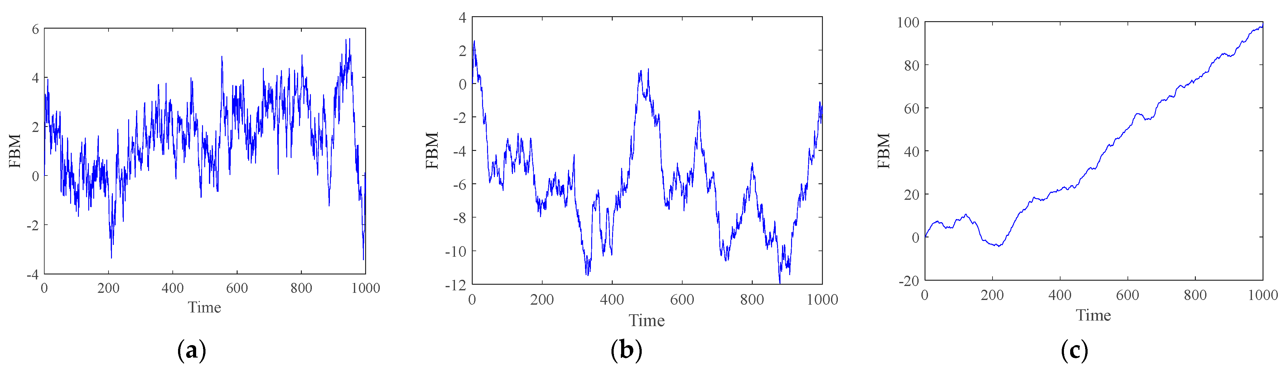
2.1. Fractional Brownian Motion

Brownian motion $B(t)$ or the Wiener process is a stochastic process with the following properties:

(1)

Its increments $B(t)-B(s),s<t$ are independent.

(2)

Its increments $B(t)-B(s),s<t$ follows a normal distribution with a zero mean.

(3)

The stochastic process is continuous.

(4)

The initial value is 0, i.e., $B(0)=0$.

To describe the fractal dimensions of some real data, Mandelbrot proposed a fractional extension of the Weiner process, i.e., FBM [23]. For the kernel function ${(t-s)}^{H-0.5}$ with $s\le t,0\le t$, FBM is described as a stochastic integral driven by Brownian motion.

$$B_H\left(t\right)=\frac{1}{\mathrm{\Gamma }\left(H+\frac{1}{2}\right)}\left\{{\displaystyle {\int }_{-\infty }^0[{\left(t-s\right)}^{H-\frac{1}{2}}-{\left(-s\right)}^{H-\frac{1}{2}}]dB\left(s\right)}+{\displaystyle {\int }_0^t{\left(t-s\right)}^{H-\frac{1}{2}}dB\left(s\right)}\right\},$$

(1)

In Figure 1, the time units represented by the X-axis are not standard time units such as seconds and minutes. This is because our research focuses on simulating the path of FBM, where each unit on the X-axis essentially represents a step or stage in the simulation process. This specific time unit selection, although non-standard, is crucial for this study as it allows us to express and analyze the temporal dynamic characteristics of FBM paths in a more precise way.

2.2. Fractional Brownian Motion

We can see from Figure 1 that the irregular behavior of FBM in a small time interval resembles the whole behavior of the FBM, such that FBM is a self-similar stochastic process [24]. The autocorrelation function (ACF) of FBM is expressed as

$$E\left(B_H\left(t\right)B_H\left(s\right)\right)=\frac{1}{2}\left(t^{2H}+s^{2H}-{\left|t-s\right|}^{2H}\right),$$

(2)

Considering $\tau =t-s\ge 0$, we have

$${ACF}_{FBM}(\tau )=\frac{1}{2}(t^{2H}+s^{2H}-{\tau }^{2H}),$$

(3)

When the Hurst index is lower than 0.5, the decaying rate of the ACF is close to exponential. In such cases, the random process is short-range dependent. Brownian motion is a special case of FBM where the Hurst exponent is 0.5 and the increments are independent. Only if the Hurst exponent is greater than 0.5 is FBM long-range dependent.

3. Degradation Modelling and Parameter Estimation

3.1. Stochastic Model Based on FBM

For a degradation process with independent increments, the degradation model is represented by [25]

$$dx\left(t\right)=\eta \left(t;\Omega \right)dt+\sigma dB\left(t\right),$$

(4)

where $dx\left(t\right)$ is the increment of the degradation process, $\eta \left(t;\Omega \right)$ is the drift coefficient, $\Omega$ is a vector with unknown parameters, and $\sigma$ is a constant diffusion coefficient.

To describe a degradation process with self-similarity and LRD characteristics, we propose that FBM replaces Brownian motion in the diffusion term. The degradation model is rewritten as

$$x\left(t\right)=x_0+\eta \left(t;\Omega \right)+\sigma B_H\left(t\right),$$

(5)

where $B_H\left(t\right)$ is FBM.

The drift coefficient $\eta \left(t;\Omega \right)$ in (5) is given by $a\phi \left(t\right)$, and $\phi \left(t\right)$ has three types of formulations [24]:

$$M_1:x\left(t\right)=x_0+at+\sigma B_H\left(t\right),$$

(6)

$$M_2:x\left(t\right)=x_0+a{t}^b+\sigma B_H\left(t\right),$$

(7)

$$M_3:x\left(t\right)=x_0+a{\mathrm{e}}^{bt}+\sigma B_H\left(t\right),$$

(8)

where M₁, M₂ and M₃ represent linear, power law and exponential drifts, respectively.

3.2. Parameter Estimation

Referring to (5), the degradation process is described as

$$x\left(k\right)=x_0+a\phi \left(t_k\right)+\sigma B_H\left(t_k\right),$$

(9)

The observed data can be expressed as $X={\left(x_1,x_2,\dots ,x_N\right)}^{\mathrm{T}}$, where $X_0$ is the initial value. The function vector and FBM vector are denoted as $\phi ={\left(\phi \left(t_1\right),\phi \left(t_2\right),\dots ,\phi \left(t_N\right)\right)}^{\mathrm{T}}$ and $B_H={\left(B_H\left(t_1\right),B_H\left(t_2\right),\dots ,B_H\left(t_N\right)\right)}^{\mathrm{T}}$. Equation (9) is rewritten as

$$X=X_0+a\phi +\sigma B_H,$$

(10)

$X$ obeys $X\sim N(X_0+a\phi ,{\sigma }^{2}Q)$, where

$$Q_{i,j}=\mathrm{cov}\left(B_H\left(t_i\right),B_H\left(t_j\right)\right)=\frac{1}{2}\left[t_i^{2H}+t_j^{2H}-{\left|t_i-t_j\right|}^{2H}\right],$$

(11)

Then, the density function of $X$ is

$$f\left(X\right)={\left(2\pi {\sigma }^2\right)}^{-N/2}{\left|Q\right|}^{-1/2}\exp \left\{\frac{-\frac{1}{2}{\left(X-X_0-a\phi \right)}^{\mathrm{T}}{Q}^{-1}\left(X-X_0-a\phi \right)}{{\sigma }^2}\right\},$$

(12)

The log-likelihood function is obtained as follows:

$$\ell \left(\Omega |X\right)=-\frac{N}{2}\ln (2\pi {\sigma }^2)-\frac{1}{2}\ln \left|Q\right|-\frac{1}{2{\sigma }^2}{\left(X-X_0-a\phi \right)}^{\mathrm{T}}{Q}^{-1}\left(X-X_0-a\phi \right),$$

(13)

The logarithmic likelihood function of parameter b in the drift function is represented as

$$\ell \left(b|X\right)=-\frac{N}{2}-\frac{1}{2}\ln \left[\det \left(2\pi Q\right)\right]-\frac{N}{2}\ln \left\{\frac{1}{N}{\left(X-X_0\right)}^{\mathrm{T}}{Q}^{-1}\left(X-X_0\right)-\frac{{\left[{\phi }^{\mathrm{T}}{Q}^{-1}\left(X-X_0\right)\right]}^2}{N{\phi }^{\mathrm{T}}{Q}^{-1}\phi }\right\},$$

(14)

To obtain the maximum likelihood estimation (MLE) of parameters $a$ and ${\sigma }^2$, the partial derivative of (21) is set to be zero, and then

$$\widehat{a}=\frac{{\phi }^{\mathrm{T}}{Q}^{-1}\left(X-X_0\right)}{{\phi }^{\mathrm{T}}{Q}^{-1}\phi },$$

(15)

$${\widehat{\sigma }}^2=\frac{1}{N}\left\{{\left(X-X_0\right)}^{\mathrm{T}}{Q}^{-1}\left(X-X_0\right)-\frac{{\left[{\phi }^{\mathrm{T}}{Q}^{-1}\left(X-X_0\right)\right]}^2}{{\phi }^{\mathrm{T}}{Q}^{-1}\phi }\right\},$$

(16)

Due to the nonlinearity of the exponential and power law drifts, obtaining the analytical forms of b is a difficult task [26]. Thus, the fminsearch function in MATLAB, employing the Nelder–Mead simplex algorithm, is designed to find the minimum of an unconstrained function. This tool is instrumental in optimizing parameters or solving problems where the objective is to minimize a specific criterion without predefined bounds [27]. The estimated values of $a$ and ${\sigma }^2$ can be calculated by (15) and (16). Computing a function vector based on such a drift function involves evaluating the drift function at various points or conditions to generate a series of values that constitute the vector.

4. Three-Step RUL Prediction Model for Roller Bearings

In this section, we propose a RUL prediction model with three different steps: degradation feature decomposition, degradation component selection and Monte Carlo RUL prediction. A flow chart of the RUL prediction model is provided in Figure 2.

In the degradation feature decomposition stage, the variational mode decomposition (VMD) algorithm is proposed to separate different degradation feature components from the vibration signal. In the degradation component selection stage, different metrics are calculated to select the best component. The selected component will be considered the HI, which is the training data for the degradation simulation driven by FBM. In the Monte Carlo RUL prediction stage, multiple degradation simulations are conducted and their mode is considered the point prediction.

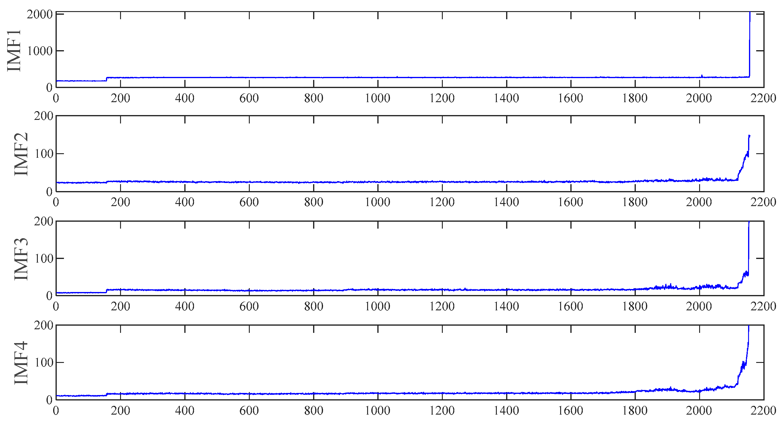
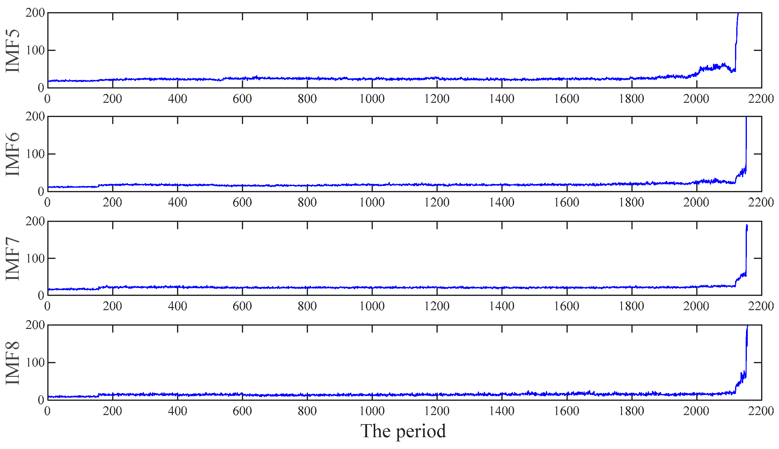
4.1. Degradation Feature Decomposition

VMD is a new method of signal decomposition, proposed by Dragomiretskiy et al. [28] in 2014. This method is to decompose the original signal into a K limited bandwidth IMFS (intrinsic mode function). It can be described as follows:

$$u_k\left(t\right)=A_k\left(t\right)\cos \left(\phi \left(t\right)\right),$$

(17)

where ${\omega }_k\left(t\right)$ is the instantaneous phase of the k-th intrinsic mode function, $A_k\left(t\right)$ is the instantaneous amplitude of the k-th intrinsic mode function and y(t) is the value of the original signal at time t, represented by the $A_k\left(t\right)$ and ${\omega }_k\left(t\right)$ determinants.

Each IMF is concentrated at the center frequency ${\omega }_k$, and the bandwidth can be estimated by its Gaussian smoothed offset signal. Due to the sparseness of VMD, it can be deemed a constrained variational problem, as expressed by

$$\underset{\left\{u_k\right\}\left\{{\omega }_k\right\}}{\min }\left\{{\displaystyle \sum _k{\Vert {\partial }_t\left[\left(\sigma \left(t\right)+\frac{j}{\pi t}\right)u_k\left(t\right)\right]e^{i-j{\omega }_{k}t}\Vert }_2^2}\right\},$$

(18)

where $\left\{u_k\right\}$ is the kth IMF and $\left\{{\omega }_k\right\}$ is the frequency center of different components. $u_k$ satisfies

$${\displaystyle \sum _{k=1}^K{u}_k}=x\left(t\right),$$

(19)

To solve the constrained variational problem, an augmented Lagrange function is introduced [29]. The problem can be written in the form

$$L\left(\left\{u_k\right\},\left\{{\omega }_k\right\},\lambda \right)=a{\displaystyle \sum _k{\Vert {\partial }_t\left[\left(\sigma \left(t\right)+\frac{j}{\pi t}\right)u_k\left(t\right)\right]e^{i-j{\omega }_{k}t}\Vert }_2^2}+{\Vert x\left(t\right)-{\displaystyle \sum _k{u}_k\left(t\right)}\Vert }_2^2+\langle \lambda \left(t\right),x\left(t\right)-{\displaystyle \sum _k{u}_k\left(t\right)}\rangle$$

(20)

where $a$ is the penalty factor and $\lambda$ is the Lagrange multiplier. The IMFs $u_k$ and corresponding center frequencies ${\omega }_k$ can be updated using (21) and (22):

$${\widehat{u}}_k^{n+1}\left(\omega \right)=\frac{x\left(\omega \right)-{\displaystyle \sum _{i=1,i<k}^K{u}_i^{n+1}\left(\omega \right)}+\frac{{\lambda }^n\left(\omega \right)}{2}}{1+2\alpha {\left(\omega -{\omega }_k^n\right)}^2},$$

(21)

$${\widehat{\omega }}_k^{n+1}=\frac{{\displaystyle \underset{0}{\overset{\infty }{\int }}\omega {\left|u_k^{n+1}\left(\omega \right)\right|}^{2}d\omega }}{{\displaystyle \underset{0}{\overset{\infty }{\int }}{\left|u_k^{n+1}\left(\omega \right)\right|}^{2}d\omega }},$$

(22)

The Lagrange multiplier $\lambda$ is updated into

$${\widehat{\lambda }}^{n+1}\left(\omega \right)={\lambda }^n\left(\omega \right)+\tau \left(x\left(t\right)-{\displaystyle \sum _k^{m+1}{\widehat{u}}_k^{n+1}\left(\omega \right)}\right),$$

(23)

The update process is carried out repeatedly until (24) is satisfied.

$${\displaystyle \sum _k\Vert {\widehat{u}}_k^{n+1}-{\widehat{u}}_k^n{\Vert }_2^2/\Vert {\widehat{u}}_k^n{\Vert }_2^2}<\epsilon ,$$

(24)

The convergence accuracy is typically set as 10-6.

4.2. Metric-Based Degradation Component Selection Algorithm

In order to choose a suitable component, monotonicity, robustness and trendability are applied for this evaluation. The monotonicity metric is described as follows [30,31,32]:

$$\{\begin{array}{l}Mo{n}_{+}\left(X\right)=\frac{No. of d/dx>0}{K-1}+\frac{No. of d^2/d^{2}x>0}{K-2}\\ Mo{n}_{-}\left(X\right)=\frac{No. of d/dx<0}{K-1}+\frac{No. of d^2/d^{2}x<0}{K-2}\end{array},$$

(25)

where $X$ is the HI (health indicator) sequence, $K$ represents the number of HI values and $d/dx=x_{k+1}-x_k$ and $d^2/d^{2}x$ denote the difference and the second-order derivatives of $X$, respectively. $No. of$ corresponds to the number of the positive and the negative difference. $Mo{n}_{+}\left(X\right)$ and $Mo{n}_{-}\left(X\right)$ represent the positive monotonicity and the negative monotonicity, respectively. The robustness is expressed as [33]

$$Rob\left(X\right)=\frac{1}{K}{\displaystyle \sum _{k=1}^K\exp \left(-\left|\frac{x_k-x_k^T}{x_k}\right|\right)}.,$$

(26)

where $x_k$ is the HI value at $t_k$ and $x_k^T$ is the mean trend value at $t_k$, calculated by smooth method. The trendability is denoted as [34]

$$Tre\left(X\right)=\frac{K\left({\displaystyle {\sum }_{k=1}^K{x}_k{t}_k}\right)-\left({\displaystyle {\sum }_{k=1}^K{x}_k}\right)\left({\displaystyle {\sum }_{k=1}^K{t}_k}\right)}{\sqrt{\left[K{\displaystyle {\sum }_{k=1}^K{x}_k^2}-{\left({\displaystyle {\sum }_{k=1}^K{x}_k}\right)}^2\right]\left[K{\displaystyle {\sum }_{k=1}^K{t}_k^2}-{\left({\displaystyle {\sum }_{k=1}^K{t}_k}\right)}^2\right]}},$$

(27)

Higher values of these metrics represent a better performance.

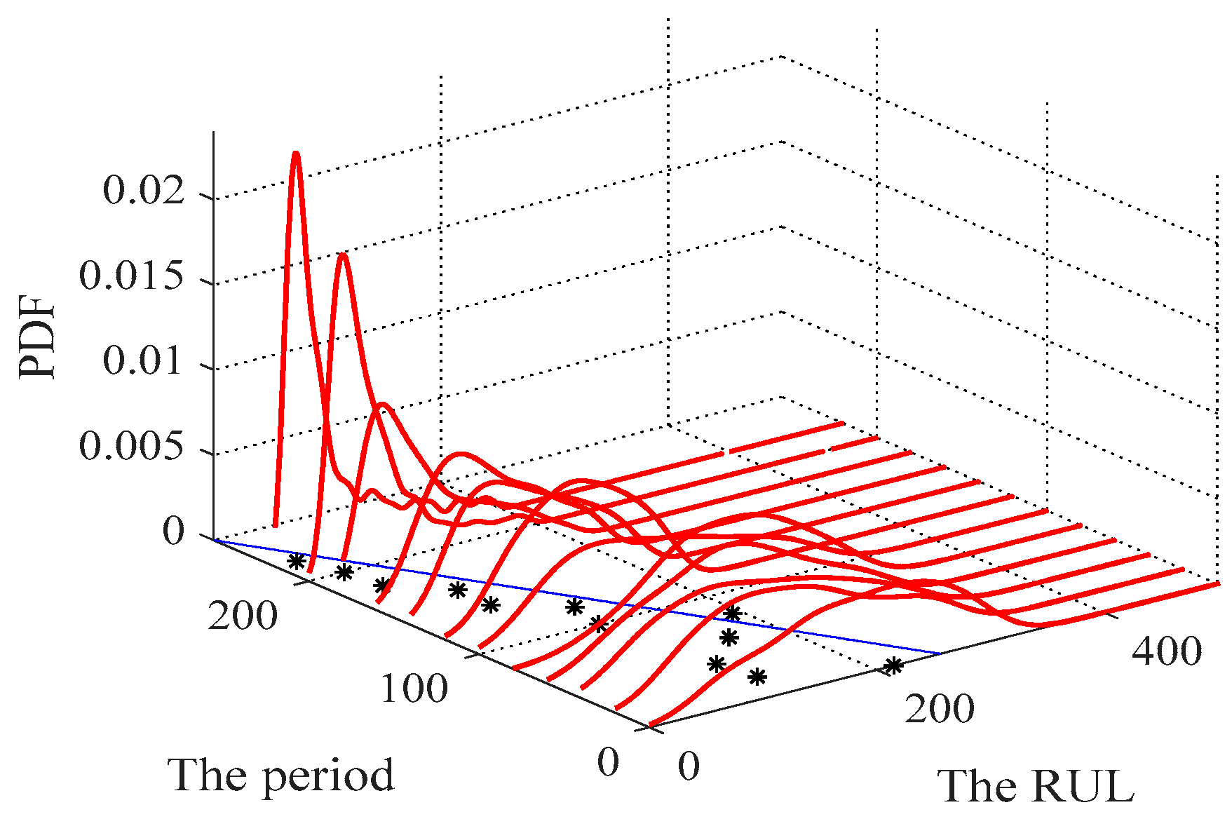
4.3. Monte Carlo Simulation for RUL Prediction

In general, the RUL at $t_k$ is defined as the first time when the degradation process reaches the failure threshold $\omega$ [35]:

$$L_k=\inf \left\{l_k>0:x(t_k+l_k)\ge \omega |x(0)=0\right\},$$

(28)

where $L_k$ represents the RUL at the kth observed time. Because the result of the model is not fixed; one calculation result is not necessarily correct. In order to come close to the actual value, the Monte Carlo method is used to predict the RUL, generating a large number of simulation paths. The mode of the Monte Carlo simulation is considered the predicted value.

The increment at interval $\mathrm{\Delta }t$ can be expressed as follows:

$$x\left(t_k+\left(j+1\right)\mathrm{\Delta }{l}_k\right)=x\left(t_k+j\mathrm{\Delta }{l}_k\right)+\sigma B_H\left(\mathrm{\Delta }{l}_k\right)+a\left[\phi \left(t_k+\left(j+1\right)\mathrm{\Delta }{l}_k\right)-\phi \left(t_k+j\mathrm{\Delta }{l}_k\right)\right]$$

(29)

The future path after j intervals at $t_k$ is

$$x\left(t_k+\left(j+1\right)\mathrm{\Delta }{l}_k\right)=x\left(t_k+j\mathrm{\Delta }{l}_k\right)+\sigma B_H\left(\mathrm{\Delta }{l}_k\right)+a\left[\phi \left(t_k+\left(j+1\right)\mathrm{\Delta }{l}_k\right)-\phi \left(t_k+j\mathrm{\Delta }{l}_k\right)\right]$$

(30)

where $B_H\left(\mathrm{\Delta }{l}_k\right)\sim \left(0,{\left(\mathrm{\Delta }{l}_k\right)}^{2H}\right)$.

The principles of the Monte Carlo RUL prediction model are depicted in Figure 3.

5. Case Study

In this section, a concrete test example is given to show the efficiency and reliability of our method.

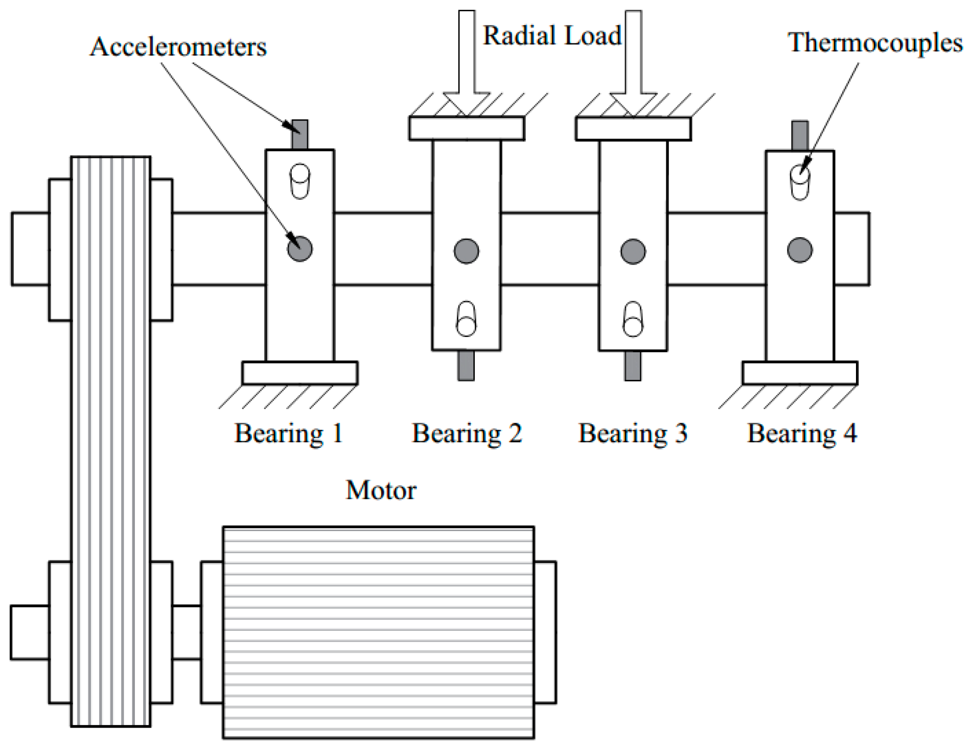
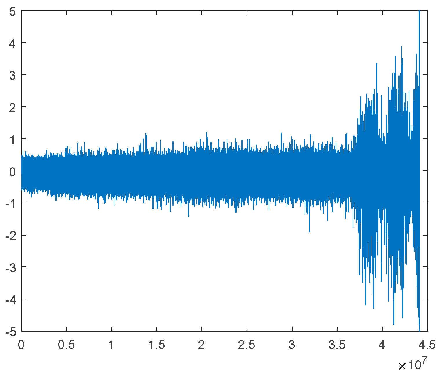
5.1. Data Description

In this section, the degradation process of a bearing data set is provided to test the validity of our proposed theory. The data were generated by the Intelligent Maintenance Systems (IMS) [36]. Four bearings are fixed on a shaft. The speed is constant at 2000 RPM. A 6000 lbs radial load is applied onto the bearing and shaft. For each bearing, data set 1 has two accelerometers, and data sets 2 and 3 have one accelerometer. The installation location is as shown in Figure 4. Each data set includes a run-to-failure experiment and its sampling rate is 20 kHz. The whole operational life data of bearing 3-Ch5 in set No. 1 is adopted. The first 43 files were recorded every 5 min and the remaining files were recorded every 10 min. The recording time was from 22 October 2003 12:06:24 to 25 November 2003 23:39:56. Figure 5 shows the vibration signal.

5.2. HI Construction of the Experimental Bearing Data

In order to extract the degradation trend, the vibration signal is decomposed into eight degradation components by VMD [37]. These degradation components are shown in Figure 6. Monotonicity, robustness and trendability are calculated for these eight components and the results are shown in

Table 1. IMFs’ performance evaluation.

Metric	IMF1	IMF2	IMF3	IMF4	IMF5	IMF6	IMF7	IMF8
Monotonicity	0.9702	1.0424	1.0135	1.0604	0.9955	1.0388	0.9811	1.0099
Robustness	0.9873	0.9593	0.9445	0.9584	0.9487	0.9389	0.9600	0.9093
Trendability	0.0900	0.4366	0.4056	0.4382	0.3557	0.3210	0.3727	0.3435

.

According to Table 1, IMF4 is selected as the training data, because it performed the best in all three indexes [38]. The failure threshold is set as $\omega =200$ and the RUL prediction starts from the 1800th time point.

5.3. RUL Prediction and Performance Evaluation

The self-similar parameter is estimated using the R/S method and its value is 0.86. Therefore, the HI is both self-similar and LRD. Other parameters are estimated by MLE. Through the Monte Carlo method, the probability density distribution (PDF) of the RUL can be simulated and the selected degradation model is M2. Obviously, the degradation process of the bearing is nonlinear and non-exponential. The utilization of M1 and M3 is inappropriate.

Figure 7 shows the PDF prediction of the proposed model. In the early stages, the distribution of its prediction results is scattered. As the RUL decreases, the distribution of the prediction results becomes more concentrated.

A Long short-term memory neural network (LSTM) model is selected for a model comparison. Its prediction results can be found in Figure 8. The RUL prediction model based on Brownian motion neglected the self-similarity and LRD of the degradation, which means it has an inferior approach.

Figure 9 shows the estimated RUL and the actual RUL for both prediction algorithms. The exponential transformed accuracy (ETA) [39] is applied to evaluate their performance. The formulas are expressed as

$$ET{A}_i=\{\begin{array}{l}\exp \left(-\ln \left(0.5\right)E{r}_i/5\right) \mathrm{if} E{r}_i\le 0\\ \exp \left(\ln \left(0.5\right)E{r}_i/20\right) \mathrm{if} E{r}_i>0\end{array},$$

(31)

where $E{r}_i$ is the percent error, defined by

$$E{r}_i=100\times \frac{ActRU{L}_i-\widehat{RU{L}_i}}{ActRU{L}_i}$$

(32)

The final score is the average of all results. A higher score represents better performance. Furthermore, the root mean squared error (RMSE) and mean absolute percentage error (MAPE) are also used for this evaluation and their results are shown in

Table 2. Predictive effect evaluation.

Model	ETA	RMSE	MAPE
M2	04713	29.8189	13.7429
M3	0.3238	52.7707	33.0301

.

6. Conclusions

In this study, we have employed the self-similarity and long-range dependence characteristics of Fractional Brownian Motion to model the uncertainty in bearing degradation. The introduction of the variational mode decomposition algorithm has enabled us to successfully separate different frequency components of the degradation, thereby enhancing the model’s interpretability and predictive accuracy. The combination of feature decomposition and component selection has proven effective in constructing the optimal health indicator, accurately capturing key aspects of the bearing degradation process. Our research not only offers a novel perspective and tool for modeling bearing degradation but also significantly supports the reliability and safety management of mechanical systems through its improved predictive accuracy.

Despite these advancements, the Gaussian assumption underlying the FBM model does not always hold, suggesting that future research might need to incorporate stochastic processes with non-Gaussian characteristics. Moreover, exploring new feature decomposition techniques and component selection strategies will be crucial in optimizing the model’s performance and extending its applicability across a wider range of scenarios. In summary, our work lays a new theoretical foundation and application framework for the development of bearing health monitoring and prediction technologies, pointing the way forward for future research and practice.

References

1. Vichare, N.M.; Pecht, M.G. Prognostics and health management of electronics. IEEE Trans. Compon. Packag. Technol. 2006, 29, 222–229. [Google Scholar] [CrossRef]
2. Lee, M.L.T.; Whitmore, G.A. Threshold Regression for Survival Analysis: Modeling Event Times by a Stochastic Process Reaching a Boundary. Stat. Sci. 2006, 21, 501–513. [Google Scholar] [CrossRef]
3. Si, X.-S.; Wang, W.; Hu, C.H.; Zhou, D.-H. Remaining useful life estimation—A review on the statistical data driven approaches. Eur. J. Oper. Res. 2011, 213, 1–14. [Google Scholar] [CrossRef]
4. Yang, G. Environmental-stress-screening using degradation measurements. IEEE Trans. Reliab. 2002, 51, 288–293. [Google Scholar] [CrossRef]
5. Chao, M. Degradation analysis and related topics: Some thoughts and a review. In Proceedings-National Science Council Republic of China Part A Physical Science and Engineering; The National Science Council: Taipei, Taiwan, 1999; Volume 23, pp. 555–566. [Google Scholar]
6. Ye, Z.S.; Xie, M. Stochastic modelling and analysis of degradation for highly reliable products. Appl. Stoch. Models Bus. Ind. 2015, 31, 16–32. [Google Scholar] [CrossRef]
7. Lee, M.Y.; Tang, J. A modified EM-algorithm for estimating the parameters of inverse Gaussian distribution based on time-censored Wiener degradation data. Stat. Sin. 2007, 17, 873–893. [Google Scholar]
8. Si, X.S.; Wang, W.B.; Hu, C.H.; Zhou, D.H.; Pecht, M.G. Remaining Useful Life Estimation Based on a Nonlinear Diffusion Degradation Process. IEEE Trans. Reliab. 2012, 61, 50–67. [Google Scholar] [CrossRef]
9. Wei, M.H.; Chen, M.Y.; Zhou, D.H. Multi-Sensor Information Based Remaining Useful Life Prediction With Anticipated Performance. IEEE Trans. Reliab. 2013, 62, 183–198. [Google Scholar] [CrossRef]
10. Bagdonavicius, V.; Nikulin, M.S. Estimation in degradation models with explanatory variables. Lifetime Data Anal. 2001, 7, 85–103. [Google Scholar] [CrossRef]
11. Park, C.; Padgett, W.J. Stochastic degradation models with several accelerating variables. IEEE Trans. Reliab. 2006, 55, 379–390. [Google Scholar] [CrossRef]
12. Wang, H.W.; Xu, T.X.; Mi, Q.L. Lifetime prediction based on Gamma processes from accelerated degradation data. Chin. J. Aeronaut. 2015, 28, 172–179. [Google Scholar] [CrossRef]
13. Ye, Z.S.; Chen, N. The Inverse Gaussian Process as a Degradation Model. Technometrics 2014, 56, 302–311. [Google Scholar] [CrossRef]
14. Pan, D.H.; Liu, J.B.; Cao, J.D. Remaining useful life estimation using an inverse Gaussian degradation model. Neurocomputing 2016, 185, 64–72. [Google Scholar] [CrossRef]
15. Li, X.Y.; Wu, J.P.; Ma, H.G.; Li, X.; Kang, R. A Random Fuzzy Accelerated Degradation Model and Statistical Analysis. IEEE Trans. Fuzzy Syst. 2018, 26, 1638–1650. [Google Scholar] [CrossRef]
16. Zhang, Z.; Si, X.; Hu, C.; Lei, Y. Degradation data analysis and remaining useful life estimation: A review on Wiener-process-based methods. Eur. J. Oper. Res. 2018, 271, 775–796. [Google Scholar] [CrossRef]
17. Beran, J. Statistics for Long-Memory Processes; Chapman & Hall: New York, NY, USA, 1994. [Google Scholar]
18. Hurst, H.E. Long Term Storage Capacity of Reservoirs. Trans. Am. Soc. Civ. Eng. 1951, 116, 770–779. [Google Scholar] [CrossRef]
19. Gui, Y.; Han, Q.K.; Chu, F.L. A vibration model for fault diagnosis of planetary gearboxes with localized planet bearing defects. J. Mech. Sci. Technol. 2016, 30, 4109–4119. [Google Scholar]
20. Mandelbrot, B.B.; Ness, J.W.V. Fractional Brownian Motions, Fractional Noises and Applications. SIAM Rev. 1968, 10, 422–437. [Google Scholar] [CrossRef]
21. Zhang, X.; Miao, Q.; Zhang, H.; Wang, L. A Parameter-Adaptive VMD Method Based on Grasshopper Optimization Algorithm to Analyze Vibration Signals from Rotating Machinery. Mech. Syst. Signal Process. 2018, 108, 58–72. [Google Scholar] [CrossRef]
22. Lei, Y.G.; Li, N.P.; Guo, L.; Li, N.B.; Yan, T.; Lin, J. Machinery health prognostics: A systematic review from data acquisition to RUL prediction. Mech. Syst. Signal Process. 2018, 104, 799–834. [Google Scholar] [CrossRef]
23. Mandelbrot, B.B.; Wallis, J.R. Robustness of The Rescaled Range R/S in The Measurement of Noncyclic Long-Run Statistical Dependence. Water Resour. 1969, 5, 967–988. [Google Scholar] [CrossRef]
24. Taqqu, M.S.; Teverovsky, V. Robustness of Whittle-type Estimators for Time Series with Long-Range Dependence. Stochastic. Models 1997, 13, 723–757. [Google Scholar] [CrossRef]
25. Beran, J.A.N. Fitting Long-Memory Models by Generalized Linear Regression. Biometrika 1993, 80, 817–822. [Google Scholar] [CrossRef]
26. Clausel, M.; Roueff, F.; Taqqu, M.S.; Tudor, C. Wavelet Estimation of the Long Memory Parameter for Hermite Polynomial of Gaussian Processes. Esaim-Probab. Stat. 2014, 18, 42–76. [Google Scholar] [CrossRef]
27. Li, M. Modeling autocorrelation functions of long-range dependent teletraffic series based on optimal approximation in Hilbert space—A further study. Appl. Math. Model. 2007, 31, 625–631. [Google Scholar] [CrossRef]
28. Chen, Y.Q.; Sun, R.T.; Zhou, A.H. An improved Hurst parameter estimator based on fractional Fourier transform. Telecommun. Syst. 2010, 43, 197–206. [Google Scholar] [CrossRef]
29. Lagarias, J.; Reeds, J.A.; Wright, M.H.; Wright, P. Convergence Properties of the Nelder—Mead Simplex Method in Low Dimensions. SIAM J. Optim. 1998, 9, 112–147. [Google Scholar] [CrossRef]
30. Dragomiretskiy, K.; Zosso, D. Variational Mode Decomposition. IEEE Trans. Signal Process. 2014, 62, 531–544. [Google Scholar]
31. Liao, L.; Jin, W.; Pavel, R. Enhanced Restricted Boltzmann Machine With Prognosability Regularization for Prognostics and Health Assessment. IEEE Trans. Ind. Electron. 2016, 63, 7076–7083. [Google Scholar] [CrossRef]
32. Zhang, H.; Chen, M.; Xi, X. Remaining useful life prediction for degradation processes with long-range dependence. IEEE Trans. Reliab. 2017, 66, 1368–1379. [Google Scholar] [CrossRef]
33. Li, Z.P.; Chen, J.L.; Zi, Y.Y.; Pan, J. Independence-oriented VMD to identify fault feature for wheel set bearing fault diagnosis of high speed locomotive. Mech. Syst. Signal Process. 2017, 85, 512–529. [Google Scholar] [CrossRef]
34. Zhang, B.; Zhang, L.J.; Xu, J.W. Degradation Feature Selection for Remaining Useful Life Prediction of Rolling Element Bearings. Qual. Reliab. Eng. Int. 2016, 32, 547–554. [Google Scholar] [CrossRef]
35. Javed, K.; Gouriveau, R.; Zerhouni, N.; Nectoux, P. Enabling Health Monitoring Approach Based on Vibration Data for Accurate Prognostics. IEEE Trans. Ind. Electron. 2016, 62, 647–656. [Google Scholar] [CrossRef]
36. Lemieux, C. Monte Carlo and Quasi-Monte Carlo Sampling; Springer Science: Berlin, Germany, 2009. [Google Scholar]
37. Wanqing, S.; He, L.; Enrico, Z. Long-range dependence and heavy tail characteristics for remaining useful life prediction in rolling bearing degradation. Appl. Math. Model. 2022, 102, 268–284. [Google Scholar]
38. Yang, F.; Habibullah, M.S.; Zhang, T.Y.; Xu, Z.; Lim, P.; Nadarajan, S. Health Index-Based Prognostics for Remaining Useful Life Predictions in Electrical Machines. IEEE Trans. Ind. Electron. 2016, 63, 2633–2644. [Google Scholar] [CrossRef]
39. Hyndman, R.J.; Koehler, A.B. Another look at measures of forecast accuracy. Int. J. Forecast. 2006, 22, 679–688. [Google Scholar] [CrossRef]
Figure 1. Simulated FBM signals: (a) H = 0.3, (b) H = 0.5, (c) H = 0.8.
Fractalfract 08 00183 g001
Figure 2. Step-by-step flowchart of the RUL prediction model.
Fractalfract 08 00183 g002
Figure 3. Plot of the principles of an RUL prediction model based on a Monte Carlo simulation.
Fractalfract 08 00183 g003
Figure 4. Bearing and sensor installation instructions.
Fractalfract 08 00183 g004
Figure 5. Original vibration signal.
Fractalfract 08 00183 g005
Figure 6. Feature extraction sequence of IMFs.
Fractalfract 08 00183 g006aFractalfract 08 00183 g006b
Figure 7. PDF prediction of the proposed model. Red line for the estimated PDF of the RUL. Asterisk for the maximum of the PDF. Blue line for the actual RUL.
Fractalfract 08 00183 g007
Figure 8. PDF prediction based on LSTM. Red line for the estimated PDF of the RUL. Asterisk for the maximum of the PDF. Blue line for the actual RUL.
Fractalfract 08 00183 g008
Figure 9. Point RUL prediction results. Asterisk for the estimated RUL. Blue line for the actual RUL. (a) PDF prediction of the proposed model (b) PDF prediction based on LSTM.
Fractalfract 08 00183 g009