Abstract
Iterative learning control is widely applied to address the tracking problem of dynamic systems. Although this strategy can be applied to fractional order systems, most existing studies neglected the impact of the system initialization on operation repeatability, which is a critical issue since memory effect is inherent for fractional operators. In response to the above deficiencies, this paper derives robust convergence conditions for iterative learning control under non-repetitive initialization functions, where the bound of the final tracking error depends on the shift degree of the initialization function. Model nonlinearity, initial error, and channel noises are also discussed in the derivation. On this basis, a novel initialization learning strategy is proposed to obtain perfect tracking performance and desired initialization trajectory simultaneously, providing a new approach for fractional order system design. Finally, two numerical examples are presented to illustrate the theoretical results and their potential applications.
1. Introduction
The concept of fractional order iterative learning control (FOILC) [1] has two meanings, where the fractional order can be derived from both the plant control system and the iterative learning law. This topic has significant research value, because fractional order systems have been verified in some important disciplines, such as secondary batteries [2] and materials science [3]; and for iterative learning control (ILC), the fractional order operator has also been proven to help improve the convergence characteristics of the system [4,5].
The initial state issue is a hot spot in ILC research [6], and its criticality can be explained from two aspects. On the one hand, the initial error significantly affects the final tracking performance; on the other hand, the possible non-repetition of the initial value also breaks the strict repeatability requirements of ILC for the plant system [7]. To the best of our knowledge, there are two main mathematical methods for dealing with the unavoidable initial errors. The first is to derive robust convergence conditions by adjusting the control structure or system assumptions [8,9,10]; and the second is to design adaptive correction algorithms to eliminate the impact of initial shift, such as initial state learning [11] and rectifying actions [12,13].
In the field of FOILC, the initial state issue has been investigated under different complex system dynamics and assumptions, such as time-delay [14], multi-agent systems [15,16], nonuniform pass lengths [17], and internal models [18]. Although most of the above learning- [19] or rectification-based [20] methods can be extended to fractional order systems, a hidden but significant issue has been neglected. Due to the historical correlation of the fractional operator, the initial values of fractional order systems are theoretically infinite dimensional [21], and a history function defined on the initialization domain is required to fully initialize the fractional order system [22]. However, in most cases, only finite dimensional initial states are considered in ILC design. If such ILC strategies are directly applied to fractional order systems, it may inevitably lead to the loss of initialization information.
The significance of considering complete initialization for fractional order systems has been revealed in both mathematics and engineering applications. For example, the initialization approach has been proven to be related to the response [23] and solution properties [24] of the system, while in material mechanics [25] and fractional order circuits [26], the significance of preprocessing has also been recognized. However, in the field of ILC, there have been no notable achievements for initialized fractional order systems. Since the initialization function is more complex than finite dimensional initial state, the analysis of ILC convergence is challenging, especially when the initialization process is perturbed or not repeated. The degree to which the initialization shift breaks the tracking performance has not been theoretically clarified. In this regard, refs. [27,28] proposed a system preconditioning strategy based on the short memory principle to improve the system performance and then derived the ILC convergence condition. However, this ILC scheme cannot achieve perfect tracking performance, and the preconditioning operation requires additional time cost.
Inspired by the existing deficiencies, this paper investigates the ILC problem of initialized fractional order systems, fully explores the impact of initialization factors on tracking performance of the iterative system, and designs control strategies to improve the convergence properties. To achieve these targets, the following methodologies are adopted. First, under the framework of initialized fractional order nonlinear system, the ILC problem is specified and the causality between system initialization and initial states is established, the operating interval is extended to the entire initialization stage. Subsequently, the convergence properties of the tracking errors are derived based on norm and contraction mapping methods. Under a close-loop -type ILC updating law, the boundedness conditions of the tracking errors are obtained, and the algorithmic factors affecting the error level are theoretically analyzed. Finally, under the condition that the initialization trajectory can be addressed, a novel initialization learning algorithm is proposed to eliminate the initialization shift and thus achieve perfect tracking performance.
The paper includes the following innovative contributions.
- (a)
- This study reveals how and to what extent system initialization weakens the ideal convergence of ILC, and a novel ILC robust convergence condition for initialized fractional order systems is strictly derived.
- (b)
- Combining the ILC tracking problem with the optimization of system initialization, a novel initialization learning strategy is proposed and applied to ensure the perfect tracking of ILC.
- (c)
- The results have broad applicability and better physical interpretability compared with existing literature, as complex system dynamics such as nonlinearity and channel noises are involved, and the connection between initialization and initial states is theoretically clarified.
The rest of this paper is organized as follows. Necessary preliminaries are presented in Section 2. The ILC problem for initialized fractional order system is stated and discussed in Section 3. Mathematical results are derived in Section 4. Numerical examples and conclusions are elaborated in Section 5 and Section 6.
2. Preliminaries
In this section, some necessary definitions and lemmas are presented. The Caputo-type fractional operator is adopted in this paper because it has integer order initial values, and is physically interpretable in real-world models [29].
Definition 1
(Fractional integral, [30]). The fractional integral of an integrable function : with order is defined as
if (1) converges pointwisely on , where denotes the Gamma function.
Definition 2
(Fractional derivative). The Caputo-type fractional derivative of a piecewise smooth function : with order is defined as
if (2) converges pointwisely on .
It can be seen from Definitions 1 and 2 that the fractional operators has nonlocal property, i.e., the derivative value of f at time t is related to the function history over the entire interval . In most FOILC studies, the fractional derivative is defined on the operating interval of the iterative system, usually a fixed . However, this approach will lead to the loss of physical information if significant history states, such as system preheating and reposition, are contained before . For a state trajectory defined on , suppose that the history states are described by the history function , where . Then, according to (2), the Caputo derivative of f containing all history information can be written as
where denotes the Caputo-type initialized fractional operator, , . The second term on the right side of (3) is actually , and the first term is called the initialization function [31]:
Thus, (3) can be rewritten as follows:
It can be seen that the initialization function actually extends the domain of the fractional operator from to , and formally maintains the consistency between the operator’s definition interval and the operating interval. Dynamic systems defined by the initialized fractional operator are called initialized fractional order systems.
The introduction of brings new complex system dynamics and challenges to control design, which will be discussed in detail in Section 3. Here, a few critical preliminaries are given. First, to evaluate the system performance over a certain interval, the definition of -norm is introduced as follows.
Definition 3.
For a function , the λ-norm is defined as:
where is a constant, denotes the infinite norm.
In addition, Lemma 1 provides the relationship between functions and their fractional integrals in the sense of ∞-norm and -norm.
Lemma 1.
Suppose that is an arbitrary fractional integrable function defined on [0, T], given a constant , then
where . Furthermore, for the λ-norm of Υ, the following inequality holds:
Proof.
Finally, the following Lemmas 2 and 3 are cited to evaluate the state of iterative systems, which are also necessary in the ILC convergence analysis.
Lemma 2
(Generalized Grönwall–Bellman inequality, [33]). Suppose that , is nonnegative and locally integrable on (), and is nonnegative, nondecreasing, continuous and no greater than a constant M on . If is nonnegative, locally integrable and satisfies
on , then
In addition, if is further nondecreasing on , then
where denotes the single-parameter Mittag–Leffler function.
Lemma 3
(see Lemma 1 and Lemma 2, [7]). For the following iterative system,
where , is the state, is the external input. Assume that the initial state is bounded, the mapping matrix Θ satisfies , where χ is a constant. If the input σ is bounded such that for some , then
- is bounded such that for some bounded .
- if .
3. Problem Statement
Many traditional ILC and FOILC problems have the following form: for a system operating repeatedly on a fixed , designing an iterative learning law, so that the input–output pair () converges to the reference pair through the iterations. To achieve this target, the existence and uniqueness assumption of the reference system, i.e., , is typically required. In this case, the convergence of and is equivalent. However, the situation is more complex for initialized fractional order systems. For a general input–output dynamic system,
the history function changes the system dynamics and breaks the input–output uniformity. This is an assignable factor for ILC issues. On the one hand, the iterative algorithm may be invalid if varies for different k, an inappropriate initialization path may also leads to an initial error and thus damages the ILC performance. On the other hand, needs to be optimized in some practical cases. For example, in battery tests (see Example 1, Section 5), resting is a notable initialization method; while in viscoelasticity, it is required to to design periodic excitation with specific amplitude and frequency [25,34]. The tracking of is usually necessary in the above scenarios.
In this paper, the following initialized fractional-order nonlinear system is considered:
where , is the state, is the input, is the output, , f, B and C have appropriate dimensions. f and g is Lipschitz continuous on with respect to t, i.e., for , . The system is initialized by a history function and the initialization function is abbreviated as . The limit value of at is assumed to be the initial state ; this is because physically the initial value should be considered as the result of the initialization operation.
Suppose that is the solution of the reference system
and meets the condition of existence and uniqueness. Then, the ILC tracking problem is to design an iterative algorithm to find a sequence, such that converges to as k increases. It can be seen from the above discussion that the history function is a generalization of the initial states. Therefore, similar to the well-known initial value issue, the initialization problems are proposed as follows and analyzed in Section 4.
- If is iteration-varying and thus leads to a non-repetitive initial shift, can ILC convergence be guaranteed? What conditions are required?
- Without considering the disturbances, if the initial history function , how to ensure that simultaneously converges to the ideal ?
4. Main Results
4.1. Bounded Tracking Error for Bounded Iteration-Varying Initialization
This section aims to derive the convergence conditions of bounded tracking errors from bounded initialization shift. More generally, the additive disturbances of the state equation and output channel are also considered. The system expression is presented as follows:
where and denote the iteration-varying shift of the state and output equations. Under an arbitrary bounded initial (), the following close-loop -type updating law is adopted for iterations:
Here, the close-loop error is introduced to enhance the robustness of the system, while the -operator is adopted to achieve better convergence performance [35]. In addition, the following assumptions are required.
- ()
- For all , is bounded on ; this assumption also indicates is bounded since .
- ()
- The tracking error of has a bounded growth speed, i.e., , where M is a constant, .
- ()
- , , and are bounded on .
The boundedness condition for tracking error of is derived in four steps below. First, the iterative relationship of the tracking errors is established based on the ILC updating law. Then, the norm-based method is adopted to evaluate the error size, and the generalized Grönwall inequality is applied to address the variable coupling. Finally, the convergence conditions for the iterative system can be found.
For and , since f and g are Lipschitz continuous, then
applying Lemma 1, (27) and (28) to (26) to eliminate f, g and the fractional operators, which yields
where
Step 2. In (29), the term needs to be substituted. For the Caputo-type fractional derivative with order , the following relationship holds:
Thus, the state shift can be expressed as
similarly to (23), in (32) can be replaced by the state equation:
Then, taking the ∞-norm to (33) and applying Lemma 1 to eliminate the fractional integral yields
where . Furthermore, since is nonnegative, and the first two terms on the right side of (34)
are nonnegative and nondecreasing with respect to t when , Lemma 2 can be applied to separate from the integral term, which yields:
To obtain the -norm of , multiplying to both sides of (35) yields
since is nondecreasing on , it is easy to see from (36) that
Step 3. Based on the results of Steps 1 and 2, the convergence property of can ultimately be derived. Applying (37) to substitute in (29) yields
Note , , then (38) can be rewritten as
where and are disturbance terms caused by internal initialization non-repetition and external channel noises:
Here, , and are bounded according to Assumptions () and (). In addition, it follows from Assumption () and (4) that
which means that is bounded as well. Since and can be arbitrarily small when is large enough, if is strictly less than 1, an appropriate can always be found so that
where is a constant. Therefore, is bounded according to Lemma 3 such that for some . Additionally, if the following assumption holds,
- ()
- ; , where ; , where .
then as .
- Step 4. The convergence results and are derived from the boundedness of . First, it is obvious that the following inequality holds according to Definition 3:which indicates that the boundedness and convergence properties of are exactly the same as . Furthermore, it follows from (37) that is bounded, i.e., for some , since , , , and are all bounded according to Assumptions (-). In addition, if Assumption () holds, then .
Finally, for the output error , it follows from the output equation of (19) that
taking the ∞-norm to both sides of (45) yields
where , . Since is bounded according to Assumption (), the boundedness and convergence conditions of is the same as that of and .
Theorem 1 and Remarks 1 and 2 can be summarized from the derivation.
Theorem 1.
For the iterative system (19), given an arbitrary bounded initial input , (). The close-loop -type updating law (20) is adopted to track the reference system (18). If
then the following conclusions hold:
- (i)
- If the assumptions (-) hold, then there are some positive constant , and , such that , , ;
- (ii)
- If the assumption () additionally holds, then .
Conclusion (i) in Theorem 1 indicates that under Assumptions (-), the tracking errors remain bounded during the iteration process. Furthermore, the size of the final tracking errors and its algorithm factors can be theoretically analyzed.
Remark 1.
It can be seen from the derivation process that, without considering the external disturbances, the tracking error level depends on the degree of shift of compared to . Taking as an example, the inequality (39) becomes
if , where . If , will decrease until , i.e., for some iteration index k, then may stop converging and remain at the level of , which is proportional to . This result is adequate for most tracking problems. In addition, since is proportional to and , and ultimately determined by according to (40), the tracking performance can be improved by reducing the initialization shift. In this regard, the preconditioning based initialization strategy [28] is noteworthy, as it can eliminate initial shift and reduce .
It can be seen from Remark 1 that the tracking performance of the iterative system can always be improved by controlling the disturbance terms, especially . The perfect tracking is achieved when the disturbance terms strictly converge to zero according to conclusion (ii). The corresponding strategies will be discussed in detail in Section 4.2. Finally, the following Remark 2 provides some explanations on the system assumptions and the selection of ILC updating law.
Remark 2.
In Assumptions () and (), the specifications about and are related to the definition of the Caputo-type fractional derivative. The boundedness of the first-order derivative is necessary to ensure the boundedness of other signals in the system, as the derivative is performed before the -order integral. Specifically, for the output channel noise , the boundedness of is crucial for obtaining a bounded output signal , since it is required to calculate the fractional derivative of the tracking error in the updating law (20). If does not meet this assumption, it is necessary to avoid using derivative operators in the ILC updating law to prevent amplifying noise.
4.2. Perfect Tracking with Initialization Learning Algorithm
As discussed in Section 3, the initialization path directly affects the dynamic characteristics of fractional-order systems. In applied disciplines such as secondary battery [36] and viscoelasticity [37], this historical hereditary effect can usually not be neglected. Identification and fitting of history function is crucial for improving system performance [21]. In this section, the ILC tracking problem is considered in conjunction with the optimization of , and a novel initialization learning algorithm is proposed to achieve perfect tracking performance.
The idea of initialization learning is inspired by the well-known initial state learning strategy [38]; the latter uses the initial output error for iteration and thereby gradually converging to the optimal . Since the history function can be viewed as an extension of the state variable x on interval , the learning algorithm for can be applied throughout the initialization stage. To achieve this target, the definitions of history function and initial state are unified into the following form:
where is called the complete history function. In addition, the system output on interval is noted as .
In order to obtain the perfect convergence condition, the non-repetitive channel disturbances and are no longer considered here. Supposing that there is no external input u on , or the input–output channel matrix . In both situations, the output error can be expressed as
where , denotes the tracking error of . Then, for an ideal reference , if the system output is measurable, Lemma 4 is proposed to eliminate the initialization shift and thereby improve the ILC performance.
Lemma 4.
Proof.
Returning to the inequality (39), since no longer exists and according to Lemma 4, then it follows from Lemma 3 that , and all converge to 0 as k grows. This indicates that, without considering external disturbances, the initialization learning strategy proposed in Lemma 4 can gradually eliminate the distortion of system dynamics caused by initialization and initial state shift, thereby achieving ideal tracking performance for the ILC scheme proposed in Section 4.1. Finally, the following Theorem 2 can be concluded.
Theorem 2.
For the iterative system (17) and reference system (18), suppose that . Given an arbitrary bounded initial input () and an arbitrary bounded and piecewise smooth initial (); for , the following close-loop -type ILC scheme with initialization learning is adopted:
If
then the following conclusion holds:
5. Numerical Examples
5.1. Example 1
A fractional capacitor is a key element in fractional order models of electrochemistry [39,40] and batteries [41]. Different from integer order capacitors, the voltage and current of a fractional capacitor exhibit a relationship of fractional derivative, and its constitutive equation is
where denotes the fractional order, is the voltage, is the current, C is a constant. A fractional capacitor is also called a constant phase element (CPE), as the phase of the impedance of fractional capacitor only depends on the the fractional exponent from the view of frequency domain [29]. The initialized fractional operator is applied here because the CPE is memorial and its performance is affected by the history voltage curve. In charging and discharging experiments related to CPE, it is usually necessary to resting the equipment to eliminate the polarization effect [42], or apply appropriate initialization stimulus to obtain the required system performance.
In this example, the voltage tracking problem of the CPE is considered, where the reference (), the order is set to be , , and the current i is chosen as the control input. To achieve this target, the close-loop -type updating law (20) is applied and the operator is selected as , which conforms to the convergence condition (47). The initial input current is set as , . The simulations are carried out in the environment of MATLAB/SIMULINK, where a number of mature open-source toolboxes [43] on fractional calculus are available. The fractional operator is implemented in the frequency domain and packaged as filter modules by adopting integer-order fitting algorithms. The objective fractional order iterative system can be easily established with the help of some other commonly used modules.
Suppose that the CPE is initialized on , the history voltage trajectory is symbolled as during the iterations. The following two initialization scenarios are concerned:
- (1)
- For a constant reference history function (), the initialization trajectory is disturbed by a iteration-varying , such that , and the initial shift . Then, are the tracking errors of and bounded? What factors are related to the size of the errors?
- (2)
- If the reference history function is set as a sinusoidal excitation signal , while the initial initialization path deviates from and further causes a significant initial shift . Then, can the initialization learning strategy (51) be applied to achieve the perfect tracking performance of , and ?
For Problem (1), the disturbed is illustrated as follows. First, since needs to be piecewise differentiable according to the Caputo definition, is assumed to be uniformly distributed on , which can be generated by the Simulink block "Uniform Random Number". The sample time is set as 0.01s. Then, is obtained by filtering through an integrator. Obviously, and are both bounded. Figure 1 shows the generation process of disturbed history function .
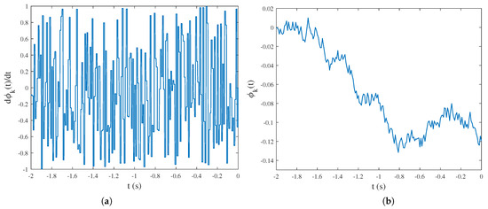
Figure 1.
Generation of the disturbance signals: (a) The first-order derivative signal of on , where , . (b) is generated by integrating the derivative signal, where , .
Set L = 0, 1, and 2, respectively, and perform 30 iterations ( means that , ); the results are shown in Figure 2. Therein, the reference input is the current trajectory corresponding to under ideal initialization condition (). From Figure 2a,c, it can be observed that the tracking error of u and i remain bounded, and the convergence process are presented in Figure 2b,d. It should be noted that fluctuates significantly near due to the iteration-varying and [28]. Thus, the root-mean-square (RMS) value of is adopted to measure the input performance on the entire , and the maximum absolute value of is applied to evaluate the output performance.
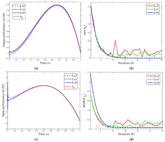
Figure 2.
System performance for different history function fluctuations (L): (a) The output performance after 30 iterations. (b) Convergence of the maximum tracking error . (c) The input performance after 30 iterations. (d) Convergence of RMS value of the input error on .
It is seen from Figure 2b,d that after about 15 iterations, the tracking error stops converging and fluctuates due to random initialization path. To clarify the impact of L on system performance, the values of and for the 16th–30th iterations are recorded, and then their RMS values are calculated, respectively. The results are stated in Table 1. The error level is positively correlated with the size of L. Since the size of L reflects the fluctuation degree of and , it can be concluded that the ILC performance depends on the shift degree of the initialization path, which has been theoretically illustrated in Remark 1.

Table 1.
The RMS value of the tracking errors for the 16th–30th iterations.
Furthermore, the initialization problem (2) is considered. Obviously, if the initial is not processed, the shift of initialization and initial value will break the convergence of the system. To obtain the perfect tracking performance, the close-loop -type ILC scheme with initialization learning (57) is applied, where , the learning is set as 0.2, which conforms to the convergence condition (58). The initialization learning is applied on , while the ILC algorithm is performed on .
Without considering other disturbances, we performed 100 iterations, and the results are shown in Figure 3. Therein, Figure 3a–c demonstrate the trajectory of , and through the iterations, and Figure 3d gives the changes in the tracking errors. It can be concluded that after 100 iterations, , and can accurately track the reference trajectories. The convergence speed of is slower, which is caused by the initial shift and evolution of the initialization path.
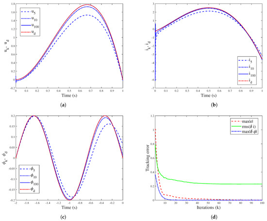
Figure 3.
System performance when applying the initialization learning strategy: (a) The tracking performance of . (b) The tracking performance of . (c) The tracking performance of . (d) Convergence of the tracking errors , , and during the iterations.
As a comparative experiment, another 100 iterations are carried out without using the initialization learning strategy (51), and the results are displayed together with the and of Figure 3, as shown in Figure 4. Obviously, the output voltage fluctuates at the initial moment without initialization learning, which is not desirable in practice. The situation with the input current is even worse, and a significant tracking error can be observed. On the contrary, when applying the ILC scheme (57), the system maintains good tracking performance, which proves the superiority of the proposed initialization learning strategy.
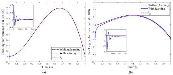
Figure 4.
System performance with/without initialization learning (): (a) The tracking performance of and the fluctuation at the initial moment. (b) The tracking performance of and the fluctuation phenomenon.
For ILC problems with initialization learning, it is significant to identify and optimize the initialization path . This issue is theoretically challenging, since is infinite dimensional, and the analytical relationship between and its response signal is relatively complex. In this regard, some discretization based data-driven strategies are notable [44,45,46], as it is difficult to apply the analytical methods. In addition, for more complex initialized fractional order systems, it may be difficult to calculate and . Nevertheless, the proposed initialization learning algorithm still has potential value, since the design of depends on various factors such as physical accessibility, operating costs, and system performance. For example, when causes an initial shift and leads to an excessive tracking error, can be designed as an achievable initialization path which satisfies . The initial shift can be eliminated by applying the initialization learning.
5.2. Example 2
In this section, a more complex system structure, which contains nonlinearity, output equation and channel disturbances, is considered:
where and are state variables, u is the control input, y is the output, and are disturbance signals. The proposed ILC strategy is applied to track the reference , where . Under the initial input , (), the close-loop -type ILC updating law (20) is adopted, where the learning gain is set to be 0.5 to satisfy the convergence conditions. Suppose that is initialized by a history function on ; similarly to Example 1, the following two initialization scenarios are considered: (1) is iteration-varying within a bounded range; and (2) the initial deviates from and needs to be addressed.
First, for scenario (1), suppose that (), is disturbed by a iteration-varying . In order to eliminate interference from other non-repetitive factors, is set to be 0, and on . The generation of is the same as that shown in Figure 1, and the sample time is set as 0.001s here. To clarify the impact of on system performance, 50 iterations are performed, respectively, for L = 20, 10, 0, and the simulation results are shown in Figure 5. It can be seen that the tracking error keeps bounded. Similarly, recording the maximum absolute error for the 16th–50th iterations and then calculating their RMS values, the results are , , . Thus, it is concluded that the the average tracking error level is positively correlated with the shift degree of the initialization path.
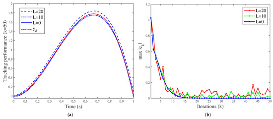
Figure 5.
System performance for different history function fluctuations (L): (a) The tracking performance after 50 iterations. (b) Convergence of the maximum tracking error .
Second, the effects of initial shift and channel disturbances on ILC performance is further investigated. Based on the first step, assuming that , , and are generated similarly as . For L = 4, 2, 0, perform 50 iterations, and the results can be seen in Figure 6. The RMS values of for the 16th–50th iterations are 0.2992 (), 0.1606 () and 0.0011 (), respectively. Combined with Figure 5b and Figure 6b, it can be concluded that the superposition of non-repetitive factors leads to an increase in average tracking error, but its overall level is still positively correlated with the amplitude (, ) and fluctuation level (, ) of the disturbances. This conclusion is consistent with the theoretical results in Section 4.
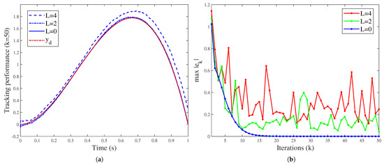
Figure 6.
System performance for different history function fluctuations, initial shifts, and channel disturbances: (a) The tracking performance after 50 iterations. (b) Convergence of the maximum tracking error .
Third, for the initialization scenario (2), suppose that on , the initial initialization path , where , . Appropriate adjustment of is necessary to eliminate the initial shift. Therefore, the reference initialization path is set to be (), such that . To apply the initialization learning algorithm, the system is assumed to have no control inputs on . Then, we adopt the learning law and perform 50 iterations; the results are presented in Figure 7. It can be seen that the initial error is gradually eliminated, and the system output achieves perfect tracking of the reference trajectory. As a comparison, Figure 7 also shows the tracking performance after 50 iterations without using initialization learning. Obvious tracking error and initial fluctuation can be observed, and the RMS value of during the iteration process is higher than that of adopting initialization learning. This proves the effectiveness of the proposed ILC strategy.
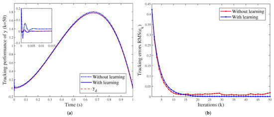
Figure 7.
System performance with/without the initialization learning strategy (): (a) The tracking performance after 50 iterations. (b) Convergence of the RMS value of the tracking error .
6. Conclusions
This paper discusses the impact of system initialization on ILC performance for initialized fractional order systems, and investigates strategies to improve system convergence. First, under the condition of iteration-varying initialization, initial shift and channel disturbances, a novel robust ILC convergence condition is strictly derived by applying the close-loop -type updating law. Second, the bounds of the tracking errors are theoretically proven to be positively correlated with the degree of initialization non-repetition. Third, a novel initialization learning algorithm is proposed to improve the initialization condition, and thereby maintain the perfect ILC tracking performance. The proposed ILC scheme includes different initialization scenarios and has good physical interpretability, and its superiority and application potential are demonstrated through the two numerical examples.
Considering the theoretical basis and physical background of system initialization, there are still some potential open issues. As mentioned in Section 5, the design, identification and optimization of initialization path is still challenging. In the field of ILC, how to combine the reset operation with system initialization is also an interesting topic.
Author Contributions
Conceptualization, X.X. and J.L.; methodology, X.X.; validation, J.L. and J.C.; investigation, X.X.; resources, J.L. and J.C.; writing—original draft preparation, X.X.; writing—review and editing, J.L. and J.C.; visualization, X.X.; supervision, J.C.; project administration, J.L.; funding acquisition, J.L. and J.C. All authors have read and agreed to the published version of the manuscript.
Funding
This work was supported in part by the National Key Research and Development Plan of China under Grant 2022YFC2403103, and in part by the National Natural Science Foundation of China under Grant 62293504, 62293500.
Data Availability Statement
No new data were created or analyzed in this study.
Conflicts of Interest
The authors declare that they have no known competing financial interests or personal relationships that could have appeared to influence the work reported in this paper.
References
- Li, Y.; Chen, Y.; Ahn, H.S.; Tian, G. A survey on fractional-order iterative learning control. J. Optim. Theory Appl. 2013, 156, 127–140. [Google Scholar] [CrossRef]
- Zeng, J.; Wang, S.; Cao, W.; Zhang, M.; Fernandez, C.; Guerrero, J.M. Improved fractional-order hysteresis-equivalent circuit modeling for the online adaptive high-precision state of charge prediction of urban-electric-bus lithium-ion batteries. Int. J. Circuit Theory Appl. 2024, 52, 420–438. [Google Scholar] [CrossRef]
- Bhangale, N.; Kachhia, K.B.; Gómez-Aguilar, J. Fractional viscoelastic models with Caputo generalized fractional derivative. Math. Meth. Appl. Sci. 2023, 46, 7835–7846. [Google Scholar] [CrossRef]
- Chen, Y.Q.; Moore, K.L. On Dα-type iterative learning control. In Proceedings of the 40th IEEE Conference on Decision and Control, Orlando, FL, USA, 4–7 December 2001; pp. 4451–4456. [Google Scholar]
- Ye, Y.; Tayebi, A.; Liu, X. All-pass filtering in iterative learning control. Automatica 2009, 45, 257–264. [Google Scholar] [CrossRef]
- Xu, J.X.; Yan, R. On initial conditions in iterative learning control. IEEE Trans. Autom. Control 2005, 50, 1349–1354. [Google Scholar]
- Meng, D.; Moore, K.L. Robust iterative learning control for nonrepetitive uncertain systems. IEEE Trans. Autom. Control 2017, 62, 907–913. [Google Scholar] [CrossRef]
- Wei, Y.S.; Chen, Y.Y.; Shang, W. Feedback higher-order iterative learning control for nonlinear systems with non-uniform iteration lengths and random initial state shifts. J. Frankl. Inst. 2023, 360, 10745–10765. [Google Scholar] [CrossRef]
- Zhang, F.; Meng, D.; Li, X. Robust adaptive learning for attitude control of rigid bodies with initial alignment errors. Automatica 2022, 137, 110024. [Google Scholar] [CrossRef]
- Shokri-Ghaleh, H.; Ganjefar, S.; Shahri, A.M. Robust convergence conditions of iterative learning control for time-delay systems under random non-repetitive uncertainties. IET Contr. Theory Appl. 2023, 17, 144–159. [Google Scholar] [CrossRef]
- Ayatinia, M.; Forouzanfar, M.; Ramezani, A. An LMI approach to robust iterative learning control with initial state learning. Int. J. Syst. Sci. 2022, 53, 2664–2678. [Google Scholar] [CrossRef]
- Chen, D.; Xu, Y.; Lu, T.; Li, G. Multi-phase iterative learning control for high-order systems with arbitrary initial shifts. Math. Comput. Simul. 2024, 216, 231–245. [Google Scholar] [CrossRef]
- Zhang, J.; Meng, D. Iterative Rectifying Methods for Nonrepetitive Continuous-Time Learning Control Systems. IEEE T. Cybern. 2023, 53, 338–351. [Google Scholar] [CrossRef] [PubMed]
- Yan, L.; Wei, J. Fractional order nonlinear systems with delay in iterative learning control. Appl. Math. Comput. 2015, 257, 546–552. [Google Scholar] [CrossRef]
- Wang, L. Iterative Learning Consensus of Fractional-Order Multi-Agent Systems Subject to Iteration-Varying Initial State Shifts. IEEE Access 2019, 7, 173063–173075. [Google Scholar] [CrossRef]
- Luo, D.; Wang, J.; Shen, D. Consensus tracking problem for linear fractional multi-agent systems with initial state error. Nonlinear Anal.-Model Control 2020, 25, 766–785. [Google Scholar] [CrossRef]
- Zhao, Y.; Li, Y.; Zhang, F.; Liu, H. Iterative learning control of fractional-order linear systems with nonuniform pass lengths. Trans. Inst. Meas. Control 2022, 44, 3071–3080. [Google Scholar] [CrossRef]
- Liu, S.; Wang, J. Analysis of iterative learning control with high-order internal models for fractional differential equations. J. Vib. Control 2018, 24, 1145–1161. [Google Scholar] [CrossRef]
- Lan, Y.H.; Wu, B.; Luo, Y.P. Finite Difference Based Iterative Learning Control with Initial State Learning for Fractional Order Linear Systems. Int. J. Control Autom. Syst. 2022, 20, 452–460. [Google Scholar] [CrossRef]
- Li, L. Rectified fractional order iterative learning control for linear system with initial state shift. Adv. Differ. Equ. 2018, 2018, 12. [Google Scholar] [CrossRef]
- Zhao, Y.; Wei, Y.; Chen, Y.; Wang, Y. A new look at the fractional initial value problem: The aberration phenomenon. J. Comput. Nonlinear Dyn. 2018, 13, 121004. [Google Scholar] [CrossRef]
- Maamri, N.; Trigeassou, J. Modelling and initialization of fractional order nonlinear systems: The infinite state approach. In Proceedings of the 10th International Conference on Systems and Control, Marseille, France, 23–25 November 2022; pp. 42–47. [Google Scholar]
- Maamri, N.; Trigeassou, J.C. A Plea for the Integration of Fractional Differential Systems: The Initial Value Problem. Fractal Fract. 2022, 6, 550. [Google Scholar] [CrossRef]
- Hinze, M.; Schmidt, A.; Leine, R.I. Numerical solution of fractional-order ordinary differential equations using the reformulated infinite state representation. Fract. Calc. Appl. Anal. 2019, 22, 1321–1350. [Google Scholar] [CrossRef]
- Remache, D.; Caliez, M.; Gratton, M.; Santos, S.D. The effects of cyclic tensile and stress-relaxation tests on porcine skin. J. Mech. Behav. Biomed. Mater. 2018, 77, 242–249. [Google Scholar] [CrossRef] [PubMed]
- López-Villanueva, J.A.; Rodríguez-Iturriaga, P.; Parrilla, L.; Rodríguez-Bolívar, S. A compact model of the ZARC for circuit simulators in the frequency and time domains. AEU-Int. J. Electron. Commun. 2022, 153, 154293. [Google Scholar] [CrossRef]
- Li, Y.; Chen, Y.Q.; Ahn, H.S. Fractional order iterative learning control for fractional order system with unknown initialization. In Proceedings of the 2014 American Control Conference, Portland, OR, USA, 4–6 June 2014; pp. 5712–5717. [Google Scholar]
- Xu, X.; Chen, J.; Lu, J. Fractional-order iterative learning control for fractional-order systems with initialization non-repeatability. ISA Trans. 2023, 143, 271–285. [Google Scholar] [CrossRef] [PubMed]
- López-Villanueva, J.A.; Rodríguez Bolívar, S. Constant phase element in the time domain: The problem of initialization. Energies 2022, 15, 792. [Google Scholar] [CrossRef]
- Kochubei, A.; Luchko, Y.; Machado, J.A.T. Handbook of Fractional Calculus with Applications-Volume 1: Basic Theory; De Gruyter: Berlin, Germany, 2019. [Google Scholar]
- Lorenzo, C.F.; Hartley, T.T. Initialization of fractional differential equations: Background and theory. In Proceedings of the 2007 Proceedings of the ASME International Design Engineering Technical Conferences and Computers and Information in Engineering Conference, Las Vegas, NV, USA, 4–7 September 2007; pp. 1325–1333. [Google Scholar]
- Lan, Y.H. Iterative learning control with initial state learning for fractional order nonlinear systems. Comput. Math. Appl. 2012, 64, 3210–3216. [Google Scholar] [CrossRef]
- Ye, H.; Gao, J.; Ding, Y. A generalized Gronwall inequality and its application to a fractional differential equation. J. Math. Anal. Appl. 2007, 328, 1075–1081. [Google Scholar] [CrossRef]
- Hosseini, S.M.; Wilson, W.; Ito, K.; Van Donkelaar, C.C. How preconditioning affects the measurement of poro-viscoelastic mechanical properties in biological tissues. Biomech. Model. Mechanobiol. 2014, 13, 503–513. [Google Scholar] [CrossRef]
- Li, Y.; Chen, Y.Q.; Ahn, H.S. Fractional-order iterative learning control for fractional-order linear systems. Asian J. Control 2011, 13, 54–63. [Google Scholar] [CrossRef]
- Hosseininasab, S.; Lin, C.; Pischinger, S.; Stapelbroek, M.; Vagnoni, G. State-of-health estimation of lithium-ion batteries for electrified vehicles using a reduced-order electrochemical model. J. Energy Storage 2022, 52. [Google Scholar] [CrossRef]
- Beltempo, A.; Bonelli, A.; Bursi, O.S.; Zingales, M. A numerical integration approach for fractional-order viscoelastic analysis of hereditary-aging structures. Int. J. Numer. Methods Eng. 2020, 121, 1120–1146. [Google Scholar] [CrossRef]
- Chen, Y.; Wen, C.; Gong, Z.; Sun, M. An iterative learning controller with initial state learning. IEEE Trans. Autom. Control 1999, 44, 371–376. [Google Scholar] [CrossRef]
- Jesus, I.S.; Tenreiro MacHado, J. Development of fractional order capacitors based on electrolyte processes. Nonlinear Dyn. 2009, 56, 45–55. [Google Scholar] [CrossRef]
- Gateman, S.M.; Gharbi, O.; Gomes de Melo, H.; Ngo, K.; Turmine, M.; Vivier, V. On the use of a constant phase element (CPE) in electrochemistry. Curr. Opin. Electrochem. 2022, 36, 101133. [Google Scholar] [CrossRef]
- Kiniman, V.; Kanokwhale, C.; Boonto, P. Modeling cyclic voltammetry responses of porous electrodes: An approach incorporating faradaic and non-faradaic contributions through porous model and constant phase element. J. Energy Storage 2024, 83, 110804. [Google Scholar] [CrossRef]
- He, X.; Sun, B.; Zhang, W.; Fan, X.; Su, X.; Ruan, H. Multi-time scale variable-order equivalent circuit model for virtual battery considering initial polarization condition of lithium-ion battery. Energy 2022, 244, 123084. [Google Scholar] [CrossRef]
- Xue, D. Fractional Calculus and Fractional-Order Control; Science Press: Beijing, China, 2018. [Google Scholar]
- Li, Y.; Zhao, Y. Memory identification of fractional order systems: Background and theory. In Proceedings of the 27th Chinese Control and Decision Conference, Qingdao, China, 23–25 May 2015; pp. 1038–1043. [Google Scholar]
- Zhao, Y.; Li, Y.; Zhou, F. Adaptive memory identification of fractional order systems. Discontin. Nonlinearity Complex. 2015, 4, 413–428. [Google Scholar] [CrossRef]
- Zhao, Y.; Wei, Y.; Shuai, J.; Wang, Y. Fitting of the initialization function of fractional order systems. Nonlinear Dyn. 2018, 93, 1589–1598. [Google Scholar] [CrossRef]
Disclaimer/Publisher’s Note: The statements, opinions and data contained in all publications are solely those of the individual author(s) and contributor(s) and not of MDPI and/or the editor(s). MDPI and/or the editor(s) disclaim responsibility for any injury to people or property resulting from any ideas, methods, instructions or products referred to in the content. |
© 2024 by the authors. Licensee MDPI, Basel, Switzerland. This article is an open access article distributed under the terms and conditions of the Creative Commons Attribution (CC BY) license (https://creativecommons.org/licenses/by/4.0/).