Abstract
To achieve high-precision deflection control of a Magnetically Suspended Control and Sensitive Gyroscope rotor under high dynamic conditions, a deflection decoupling method using Quantum Radial Basis Function Neural Network and fractional-order terminal sliding mode control is proposed. The convergence speed and time complexity of the neural network controller limit the control accuracy and stability of rotor deflection under high-bandwidth conditions. To solve the problem, a quantum-computing-based structure optimization method for the Radial Basis Function Neural Network is proposed for the first time, where the input and the center of hidden layer basis function of the neural network are quantum-coded, and quantum rotation gates are designed to replace the Gaussian function. The parallel characteristic of quantum computing is utilized to reduce the time complexity and improve the convergence speed of the neural network. On top of that, in order to further address the issue of input jitter, a fractional-order terminal sliding mode controller based on the Quantum Radial Basis Function Neural Network is designed, the fractional-order differential sliding mode surface and the fractional-order convergence law are proposed to reduce the input jitter and achieve finite-time convergence of the controller, and the Quantum Radial Basis Function Neural Network is used to approximate the residual coupling and external disturbances of the system, resulting in improving the rotor deflection control accuracy. The semi-physical simulation experiments demonstrate the effectiveness and superiority of the proposed method.
1. Introduction
Magnetically Suspended Control Sensitive Gyroscope (MSCSG) is a new type of actuator for spacecraft attitude control [1]. Unlike existing single-functional magnetic suspension control moment gyroscopes or magnetic suspension rate gyroscopes, the MSCSG has the outstanding advantage of simultaneous control and sensing and has great potential for high-accuracy control. However, there are challenges and difficulties in realizing high-precision control of MSCSG. Some of the key factors that affect the high-precision and high-bandwidth control of MSCSG are the problems of constant speed, suspension accuracy, and stability of the high-speed magnetic suspension rotor. The magnetic suspension rotor is a complex system with highly dynamic, nonlinear, and strongly coupled characteristics [2]. When subjected to external disturbances, the rotor will generate displacement, affecting the suspension accuracy of the rotor. Therefore, external disturbances must be suppressed. When controlling the high dynamic deflection of the rotor to output control moment, the real-time performance of the control system will affect the moment accuracy. There are currently various control methods for magnetically suspended rotor decoupling control, such as PID decoupling control [3], sliding mode control [4], and self-adaptive decoupling control [5]. In addition, there are decoupling control methods that combine traditional methods with neural networks [6].
Ren analyzed the effect of cross-coupling and feedforward channel delays on the stability of PID cross-feedback decoupling control [7] and proved that the cross-coupling channel delay is the main factor affecting stability. However, he did not propose an effective method of delayed compensation.
Xia proposed a feedforward internal model decoupling control method for magnetically suspended rotor [8]; however, the model’s accuracy limits the control accuracy at high bandwidths.
Wang proposed a control method for the magnetically suspended rotor using active disturbance rejection control (ADRC) [9], which achieved high-accuracy control of the deflection channel under external perturbation conditions, but the adjustment of the controller parameters was complicated. Yin proposed a state feedback self-adaptive disturbance rotor control method, but did not consider the decoupling accuracy problem under high-dynamic conditions. Reference [10] proposed an RBF neural network ADRC method, which achieved self-adaptive parameter adjustment through neural networks and improved the system’s robustness. However, all three methods adopted active disturbance rejection control (ADRC), which makes it difficult to adjust the parameters [11]. Moreover, the second-order extended state observer essentially belongs to an integral system [12,13], which will cause a lag effect on the system, which is inadvisable for high-dynamic disturbance observation and control.
Sliding mode control (SMC) can effectively address high-precision control under external disturbance conditions [14]. Dou proposed a rotor neural network sliding mode control method to improve system robustness [15]. Zheng proposed an SMC method for a satellite magnetically suspended rotor [16]. Wang proposed a terminal SMC method for magnetically suspended flywheels [17]. Some studies focus on improving the performance of the controller by using fractional-order theory [18,19]. Zhang proposed a fractional-order PD attitude control method for spacecraft with flexible attachments [20]. Yu proposed a model-free fractional-order sliding mode controller with a nonlinear disturbance observer that has good dynamic response and strong robustness [21]. These methods achieved convergence within a limited time; however, the problem of input jitter under high dynamic conditions remains [22].
Neural network control has potential in the field of nonlinear system control by general approximation of unknown functions. The Radial Basis Function Neural Network (RBF-NN) is a multi-layer feed-forward neural network with a simple structure that can approximate nonlinear functions with arbitrary accuracy and is widely used in the control of nonlinear systems [23,24]. However, the network structure and time complexity constraints unavoidably affect the approximation performance under high-dynamic disturbances [25]. Some scholars have improved the approximation accuracy and dynamic performance of neural networks by introducing the idea of quantum computing for optimizing network parameters and structures [26,27]. L. proposed a BP neural network based on universal quantum gates, which improved the convergence rate of the network [28]. Li proposed a quantum neural network model based on controllable Hadamard gates, which improved the approximation accuracy of the network [29]; Ye used quantum evolutionary algorithms for parameter tuning of neural network PID controllers, achieving certain effects [30]. As for the Quantum Radial Basis Function Neural Network (QRBF-NN), Liu proposed a method to improve RBF using quantum coding, and simulations showed that QRBF-NN outperforms RBF in image recognition [31]. Shao proposed two quantum algorithms to train RBF networks, which sped up the training [32]. However, these methods only improve the network performance based on traditional quantum gate circuit neural networks without improving the network structure, resulting in limited effects for high-bandwidth nonlinear systems. Due to the high dynamic characteristics of MSCSG rotors, the real-time performance of traditional neural networks further magnifies the impact on control accuracy.
In summary, the traditional MSCSG rotor neural network control method has the following problems: (1) High network time complexity, which affects the high-frequency deflection control accuracy of the rotor. (2) Controller design needs to be further optimized to speed up the convergence speed and reduce the input jitter. To solve these problems, in this paper, a decoupling control method for rotor deflection based on QRBF-NN and terminal sliding mode control is proposed. Firstly, the RBF neural network structure is optimized using the idea of quantum computing. Exploiting the parallel characteristic of quantum computing, the time complexity of the network is reduced, thereby enhancing the approximation accuracy under high-bandwidth conditions. Secondly, a fractional-order terminal sliding mode controller based on QRBF-NN is designed, incorporating a fractional-order sliding surface and fractional-order approaching law to reduce input jitter and improve control accuracy. Finally, the effectiveness and superiority of the proposed method are validated through semi-physical simulation.
The paper is organized as follows: Section 2 describes the modeling of MSCSG. Section 3 provides the QRBF-NN and controller design and two relevant theorems. Section 4 presents the simulations and comparisons. Section 5 draws a conclusion of the research.
To the best of the authors’ knowledge, the result presented in this paper is the first attempt in the literature to accomplish MSCSG rotor high-precision deflection decoupling control using QRBF-NN.
2. Dynamic Molding of In-Orbit MSCSG
MSCSG utilizes a Lorentz force magnetic bearing (LFMB) as a moment actuator to achieve radial deflection of the rotor, and its principles of operation are shown in Figure 1. The LFMB coordinate system, defined by OXgYgZg, is fixed to the LFMB stator, and O is the centroid of the spherical rotor. The rotor coordinate system OXrYrZr is tied up with the magnetic suspension rotor, but cannot rotate around OrZr. When the rotor does not deflect, each axis of OrXrYrZr coincides with that of OXgYgZg. The rotor deflects at angles of α and β around OXg and OYg.
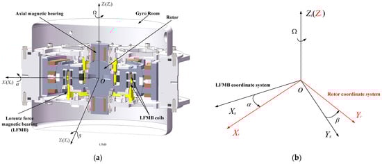
Figure 1.
Schematic diagram of MSCSG structure: (a) section view of MSCSG, (b) coordinate system definition.
When the coil is perpendicular to the magnetic field and a current is passed through it, an amperometric force perpendicular to the direction of the coil and the magnetic field will be generated in the upper and lower parts of the coil, respectively. The magnitude of the force can be expressed as
where fx, fy are ampere forces in the Xg- and Yg-axis directions, respectively. N is the number of turns in the coil of LFMB; B is the magnetic field strength; L is the length of the coil; I1, I2 are the coil driving currents in the positive and negative directions of the Xg-axis; respectively; and I3, I4 are the same currents of the Yg-axis, respectively. Suppose that ; when coils of opposite directions are fed with equal currents of opposite directions, the coils will produce equal and opposite ampere forces. It can be inferred that the LFMB provides deflection moments in the X and Y directions as follows:
where lm represents the stator radius of the LFMB.
Suppose that each axis of OXgYgZg coincides with that of the spacecraft coordinate system. The angular velocity of the LFMB coordinate system with respect to the inertial coordinate system is , and the angular velocity of the rotor coordinate system with respect to the LFMB coordinate system is projected in the LFMB coordinate system as . The projection of the angular velocity of the rotor relative to the inertial space in the rotor coordinate system can be expressed as
where represents the transformation matrices from the LFMB coordinate system to the rotor coordinate system. Since the angular velocity components of the rotor coordinate system around the stator coordinate system are , and 0, respectively, one has . Suppose that .
In actual engineering, α and β are less than 10−3 rad:
One has
Ir, Iz denote the rotor moment of inertia in the axial and radial directions around the stator, respectively. The rotor angular momentum is
where , and Ω is the constant rotational speed of the rotor about the z-axis.
The dynamic equation of the magnetically suspended rotor in the rotor coordinate system can be expressed as
where Mr is the total external moment applied to the rotor. is the rate of change in the rotor angular momentum.
The rotor angular momentum and its rate of change can be written as
According to Euler’s dynamics equation, the in-orbit MSCSG radial dynamics model can be expressed as
where dx and dy represent the unknown disturbances in the Xg- and Yg-axis directions, respectively.
3. Design of QRBF-NN and Controller
3.1. Quantum-Computing-Based Structure Optimization Method of RBF-NN
As shown in Figure 2, an n-dimensional input vector it can be transformed into a diagonal matrix in an n-dimensional Hilbert space.
where
where is the quantum phase angle for the i-th input.
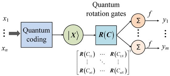
Figure 2.
Schematic diagram of QRBF.
For an RBF neural network with n inputs and N neurons, the hidden layer center can be expressed as
Through quantum coding, the hidden layer center can be rewritten as
where
The quantum rotation gate is designed to replace the hidden layer center by introducing quantum computing concepts. The quantum rotation gate can be expressed as
where
In a traditional RBF neural network, the role of the hidden layer is to map a vector from a low-dimensional m to a high-dimensional n, making linearly inseparable cases in low dimensions become linearly separable in high dimensions. The output of the hidden layer can be expressed as
where denotes the network input vector, n, m, respectively represents the number of nodes in the input layer and hidden layer, hi represents the Gaussian basis function, and stands for the network product-width.
The input after undergoing quantum rotation gate transformation can be expressed as
where
The sum of the probability amplitudes of is used as the neuron output. Define the output of the jth neurons as
The definition domain of is [−n, n]. A non-linear mapping can be constructed:
The output of the hidden layer in QRBF-NN can be written as
The output of the QRBF-NN can be expressed as
The following proves that the input to output of QRBF-NN is a continuous mapping.
For a real-valued input, and , since is a continuous mapping.
Theorem 1.
The QRBF-NN designed in this paper can approximate any continuous function uniformly on any compact set and any measurable function arbitrarily.
Definition 1.1.
K: is an integrable bounded function such that K is continuous and; the family Sk consists of functions g: represented by
where for . denotes the usual spaces of R-valued maps f defined on Rr.
Lemma 1.1.
Let μ be a finite measure on Rr, , and the family Sk is dense in with respect to the metric ρμ defined by [33]:
Lemma 1.1 establishes that under certain mild conditions on the kernel function, networks with one hidden layer and the same smoothing factor in each kernel are broad enough for universal approximation. We will use this lemma to prove that QRBF-NN has similar properties.
Proof of Theorem 1.
Firstly, we prove that the mapping from input to output of a QRBF-NN is a continuous function.
, , , and one has .
, , and when , one has .
Since , and ; when , one has , which means the mapping from input to output of a QRBF-NN is a measurable continuous function from .
Secondly, we prove that satisfies the conditions on K in Definition 1.1.
Let , . It is clear that is in the range [0,4π]; thus, is in the range , which means .
The proof is finished. □
Theorem 2.
The QRBF-NN designed in this paper outperforms RBF-NN in terms of time complexity when the neuron number N is large enough.
Proof of Theorem 2.
The kernel function of RBF-NN can be expressed as
The kernel function of RBF-NN can be expressed as
Suppose t1 is one unit of CPU time for addition or subtraction, t2 is one unit of CPU time for multiplication or division, t3 is one unit of CPU time for exponentiation, and t4 is one unit of CPU time for sine or cosine operation. Nested loops are avoided because QRBF-NN uses matrix operations. Then, the time complexity of one kernel operation of RBF-NN and QRBF-NN can be written as
It seems that the time complexity of a kernel operation of QRBF-NN is larger than that of RBF-NN. However, due to the parallel nature of quantum computing, operations on N neurons in QRBF-NN are simultaneous while operations on N neurons in RBF-NN are cyclic. Thus, for an RBF-NN with N neurons, the time complexity is
while . One has
if and only if
which is easy to achieve when N is large enough.
The proof is finished. □
Moreover, since the definition domain of Cij is [−0, 2π], which covers the whole range of rotation angles, Cij does not have to be adjusted. The only parameter that needs to be adjusted in QBF-NN is K, while Ci, , and K are the parameters to be adjusted in RBF-NN.
It can be obtained that the QRBF-NN has a lower time complexity than RBF-NN, and as the number of network neurons increases, the gap will become more and more obvious.
3.2. Design of Fractional-Order Terminal Sliding Mode Controller Based on QRBF-NN
Aiming at the strong coupling, high dynamics, and nonlinearity of the magnetic suspended rotor system, based on the use of QRBF to approximate the system disturbances, we propose a terminal sliding mode controller based on the combination of a fractional-order sliding mode surface and a fractional-order convergence law in order to achieve system decoupling and to reduce the input jitter.
Combining the perturbation terms, one obtains
As shown in Figure 3, feedforward compensation is used to decouple the two degrees of freedom of rotor deflection. The control system diagram is shown Figure 4.
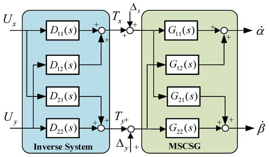
Figure 3.
Feedforward compensation decoupling.
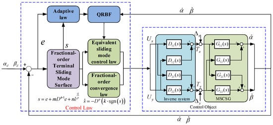
Figure 4.
Control system diagram.
Here,
The decoupled system can be written as
where Δx and Δy are the disturbances of the Xg-axis and Yg-axis, respectively. QRBF-NN is used to approximate :
Taking the example of deviation around the Yg-axis,
where εx represents the network approximation error. Then, the output of the RBF network can be expressed as
The ideal steering angle tracking command is βb and the tracking error is defined as e = βb − β. To achieve fast convergence of the system in finite time, the fractional-order terminal sliding mode surface is designed as
where p and q are odd numbers and p > q, m and n are the sliding mode surface parameters and m > 0 and n > 0, and r is the differential order and satisfies . According to the definition of RL fractional-order differentiation,
One has
Assuming that s = 0, the equivalent control law can be obtained as follows:
The fractional-order sliding mode reaching law is designed as follows:
where k is the reaching law parameter, and t is the differential order and satisfies . The control law can be expressed as
where
Define the Lyapunov function as
where γ > 0.
Taking the derivative of Equation (49) yields
Designing the adaptive law as
one has
Since , when , .
It can be seen that for unknown external disturbances d, the system can be stabilized as long as k is selected. There is no restriction on the bandwidth or derivative of d. The proposed method can take full advantage of the high-bandwidth moment output by MSCSG and the fast convergence property of the QRBF to suppress spacecraft micro-vibrations.
4. Semi-Physical Simulation
4.1. Simulation Analysis of QRBF-NN Approximation Performance
Firstly, simulations were conducted to compare the approximation accuracy and approximation speed of RBF and QRBF. The objective function was set as a sine function with an amplitude of 1 and frequencies of 1 Hz, 10 Hz, and 100 Hz. The training was conducted continuously for 20 iterations, with the root mean square error of approximation error used as the criterion. The results are shown in Table 1 and Table 2.

Table 1.
Approximation error of RBF-NN and QRBF-NN.
Table 2.
Time complexity of RBF-NN and QRBF-NN.
It can be observed from Table 1 that as the bandwidth of the objective function increases, the approximation error of both neural networks also increases. However, when the bandwidth of the objective function is set at 1 Hz, 10 Hz, and 100 Hz, QRBF-NN consistently exhibits lower approximation errors compared to the traditional RBF-NN network.
It can be observed from Table 2 that when the bandwidth of the objective function is set at 1 Hz, 10 Hz, and 100 Hz, QRBF-NN consistently exhibits lower time complexity compared to the traditional RBF-NN.
Secondly, simulations were conducted to compare the robustness of RBF-NN and QRBF-NN. The objective function was defined as a sine function with an amplitude of 10 and a frequency of 1 Hz. At 1 s, a sine function with an amplitude of 20 and a frequency of 50 Hz was added. At 4 s, a sine function with an amplitude of 15 and a frequency of 100 Hz was added. At 8 s, a sine function with an amplitude of 30 and a frequency of 30 Hz was added. The results are shown in Figure 5 and Figure 6. The red line represents the true value and the blue line represents the approximation.
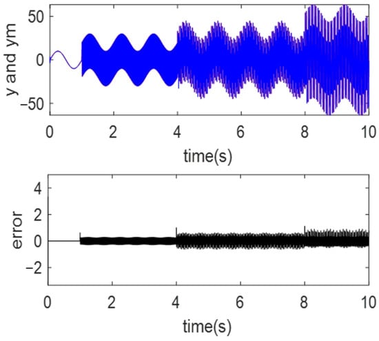
Figure 5.
Approximation and error of QRBF-NN.
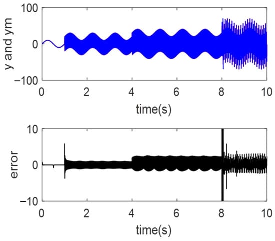
Figure 6.
Approximation and error of RBF-NN.
4.2. Comparison of Control Performance for QRBF-NN and RBF-NN
The parameters of the MSCSG and controller are shown in Table 3.
Table 3.
MSCSG parameters.
Simulations were conducted to compare the decoupling control performance of RBF-NN and QRBF-NN. The simulations were performed using the following three control methods.
Method 1: RBF-NN method in [10] (RBF-NN and ADRC);
Method 2: QRBF-NN combined with sliding mode control (QRBF-NN and SMC);
Method 3: QRBF-NN combined with fractional-order terminal sliding mode control (QRBF-NN and FOSMC).
Firstly, the decoupling performance of the three methods was verified. The rotor deflection command around the Xg-axis is a sinusoidal signal with an amplitude of 1° and a period of 0.75π. Additionally, at 0.5 s, the rotor deflection command around the Yg-axis is a step signal with an amplitude of 1°.
From Figure 7, it can be observed that the rotor controlled by method 1 still exhibits coupling between the two degrees of freedom, while the rotor controlled by methods 2 and 3 does not exhibit coupling. The performance comparison of the three methods is shown in the Table 4.
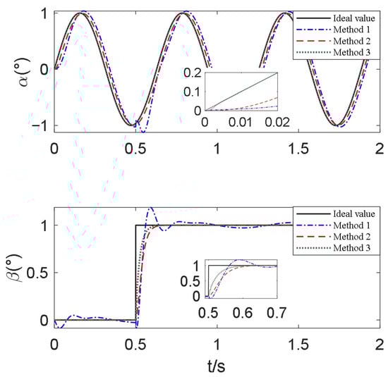
Figure 7.
Comparison of rotor deflection decoupling performance of 3 methods.
Table 4.
Control performance comparison.
As for the settling time, the rotor deflection angles controlled by method 1 continue to fluctuate in a small range, whereas the signal controlled by methods 2/3 stabilized by 0.7 s. Due to the faster convergence speed of the fractional-order sliding mode controller, method 3 tracks the reference signal faster than method 2 while also having a smaller phase difference. As for overshoot, the rotor deflection angle controlled by method 1 has 22% overshoot while methods 2 and 3 do not. Due to the better approximation performance of QRBF-NN compared to RBF-NN, method 2 achieves higher control accuracy than method 1.
Secondly, the control accuracy of the three methods was verified. The rotor deflection command was a sinusoidal signal with an amplitude of 0.5° and a frequency of 20 Hz around the Xg-axis. At 2 s, a sinusoidal signal with an amplitude of 1° and a frequency of 25 Hz was added. At 5 s, a sinusoidal signal with an amplitude of 0.5° and a frequency of 50 Hz was added. At the same time, the rotor was subjected to an external disturbance of which the amplitude was 0.02 N and the frequency was 40 Hz, and another external disturbance of which the amplitude was 0.03 N and the frequency was 75 Hz in the Xg-axis. The rotor deviation angles and errors controlled by three methods are shown in Figure 8, Figure 9 and Figure 10.
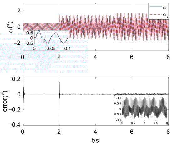
Figure 8.
Rotor deflection angle and error controlled by method 1.
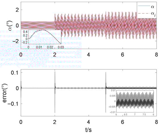
Figure 9.
Rotor deflection angle and error controlled by method 2.
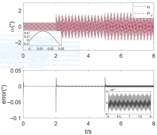
Figure 10.
Rotor deflection angle and error controlled by method 3.
It can be seen from Figure 8 that the rotor controlled by method 1 tracked the reference signal at 0.1 s and had a stable deflection angle error of [−0.008, 0.012]°.
It can be seen from Figure 9 that the rotor controlled by method 2 tracked the reference signal at 0.02 s and had a stable deflection angle error of [−0.006, 0.009]°.
It can be seen from Figure 10 that the rotor controlled by method 3 tracked the reference signal at 0.01 s and had a stable deviation angle error of ±0.005°. Compared with method 1 and method 2, method 3 has advantages in terms of reference tracking speed and control accuracy. At the same time, the reference tracking speed and control accuracy of method 2 are higher compared to method 1, which proves the superiority of QRBF-NN.
4.3. Experimental Analysis of MSCSG
The MSCSG laboratory setup is shown in Figure 11. The rotor deflection command around the Xg-axis is a sinusoidal signal with a frequency of 120 Hz while remaining stationary around the Yg-axis. We collected the rotor deflection signals for offline simulation experiments.
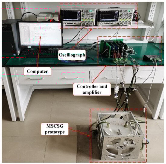
Figure 11.
MSCSG laboratory setup.
As can be seen from Figure 12, due to the coupling of the two degrees of freedom of rotor deflection, when the rotor is controlled to deflect along the Yg-axis, the rotor will also deflect along the Yg-axis, and the Yg-axis phase is 90 degrees behind the x-axis. The Fourier transform of β shows that the amplitude of the deflection frequency of β is 0.12.
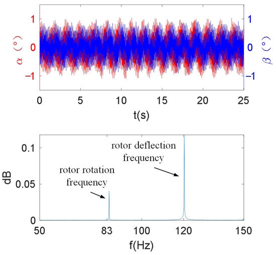
Figure 12.
Two degrees of freedom of rotor deflection angles controlled by the traditional method.
As can be seen from Figure 13, the two-degree-of-freedom coupling of the rotor deflection controlled by the new method is reduced. The Fourier transform of β shows that the amplitude of the deflection frequency of β is 0.05, which decreases by 58.3% compared to the traditional method. Meanwhile, the α controlled by the proposed method is smoother than that of the traditional method, proving that the proposed method is better than the traditional method in terms of control accuracy and decoupling performance.
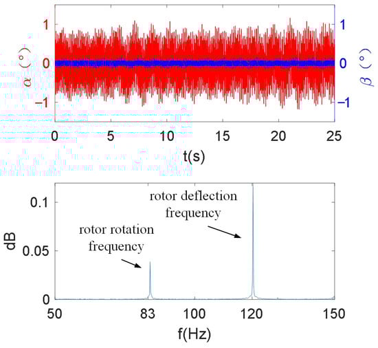
Figure 13.
Two degrees of freedom of rotor deflection angles controlled by the proposed method.
5. Conclusions
In this paper, a decoupling control method for MSCSG rotor deflection based on QRBF-NN and fractional-order terminal sliding mode control is proposed.
A quantum-computing-based optimization method for the structure of the RBF-NN is proposed for the first time. The following two conclusions are drawn: (1) the QRBF-NN is able to approximate continuous functions with arbitrary accuracy; (2) the QRBF-NN outperforms the conventional RBF-NN in terms of time complexity.
Building upon this, a fractional-order terminal sliding mode control method based on QRBF-NN is proposed. The fractional-order sliding surfaces and approaching laws are designed. The simulation results show that (1) the QRBF-NN can accurately approximate perturbations while reducing latency; (2) the proposed method can realize high-precision decoupling control of MSCSG rotor.
In the future, we will further theoretically prove the generalization of QRBF-NN and the stability of the QRBF-NN fractional-order controller. And we will prove its effectiveness and advancement through more experiments to promote its application.
Author Contributions
Methodology, Y.R. and L.L.; Software, W.W. and L.W.; Validation, W.P. All authors have read and agreed to the published version of the manuscript.
Funding
National Natural Science Foundation of China: 52075545.
Data Availability Statement
Data are contained within the article.
Conflicts of Interest
The authors declare no conflicts of interest.
References
- Yin, Z.; Cai, Y.; Ren, Y.; Wang, W. A Measurement Method of Torque Coefficient for Magnetically Suspended Control and Sensitive Gyroscope. IEEE Sensors J. 2021, 21, 14767–14775. [Google Scholar] [CrossRef]
- Li, L.; Ren, Y.; Wang, W.; Wang, L.; Yin, Z.; Yu, C. Spacecraft Attitude Measurement and Control Integration Using a Novel Configuration of Variable Speed Magnetically Suspended Control and Sensing Gyroscope. IEEE Sensors J. 2023, 23, 9359–9369. [Google Scholar] [CrossRef]
- Numanoy, N.; Srisertpol, J. Vibration Reduction of an Overhung Rotor Supported by an Active Magnetic Bearing Using a Decoupling Control System. Machines 2019, 7, 73. [Google Scholar] [CrossRef]
- Barambones, O.; Alkorta, P. Position Control of the Induction Motor Using an Adaptive Sliding-Mode Controller and Observers. IEEE Trans. Ind. Electron. 2014, 61, 6556. [Google Scholar] [CrossRef]
- Liu, X.; Ma, X.; Zheng, S.; Zhou, J.; Chen, Y. Feedback Linearization and Robust Control for Whirl Mode with Operating Point Deviation in Active Magnetic Bearings-Rotor System. IEEE Trans. Ind. Electron. 2022, 70, 7673–7682. [Google Scholar] [CrossRef]
- Wang, X.; Dai, X. An Improving Method to Decoupling and Linearization of Induction Motor Based on Neural Network Inverse. Trans. China Electrotech. Soc. 2018, 10, 4–31. [Google Scholar]
- Chen, X.; Ren, Y.; Wang, W.; Cai, Y. Rotation Modes Stability Analysis and Phase Compensation for Magnetically Suspended Flywheel Systems with Cross Feedback Controller and Time Delay. Math. Probl. Eng. 2016, 2016, 3783740. [Google Scholar]
- Xia, C.; Cai, Y.; Ren, Y.; Wu, D.; Wang, Y. Feedforward decoupling and internal model control for rotor of magnetically suspended control and sensing gyroscope. J. Beijing Univ. Aeronaut. Astronaut. 2017, 44, 480–488. [Google Scholar]
- Wang, P.; Wang, H.; Ren, Y. Decoupling Control and Disturbance Rejection of Radial Rotor System in Magnetically Suspended Control Moment Gyro Based on ADRC. Ordonance Ind. Autom. 2015, 34, 59–63. [Google Scholar]
- Li, L.; Ren, Y.; Chen, X.; Yin, Z. Design of MSCSG control system based on ADRC and RBF neural network. J. Beijing Univ. Aeronaut. Astronaut. 2020, 46, 1966–1972. [Google Scholar]
- Chu, M.; Chen, G.; Huang, F.J.; Jia, Q.X. Active Disturbance Rejection Control for Trajectory Tracking of Manipulator Joint with Flexibility and Friction. Appl. Mech. Mater. 2013, 325–326, 1229–1232. [Google Scholar] [CrossRef]
- Zhang, H.; Zhao, S.; Gao, Z. An active disturbance rejection control solution for the two-mass-spring benchmark problem. In Proceedings of the 2016 American Control Conference (ACC), Boston, MA, USA, 6–8 July 2016. [Google Scholar]
- Jin, H.; Chen, Y.; Lan, W. Linear Active Disturbance Rejection Control with Partially Canceling Estimated Total Disturbance. In Proceedings of the IEEE International Conference on Real-Time Computing and Robotics, Irkutsk, Russia, 4–9 August 2019. [Google Scholar]
- Zhang, X.; Su, H.; Lu, R. Second-Order Integral Sliding Mode Control for Uncertain Systems with Control Input Time Delay Based on Singular Perturbation Approach. IEEE Trans. Autom. Control. 2015, 60, 3095–3100. [Google Scholar] [CrossRef]
- Dou, Z.; Yang, L.; Ren, Z. Decoupling control of maglev rotor’s gyro effect supported by nonlinear force. Mech. Sci. Technol. Aerosp. Eng. 2023, 42, 1392–1401. [Google Scholar] [CrossRef]
- Zheng, C. Research on Unbalance Disturbance Control Method of Magnetic Bearing Rotor System Aboard Satellite; Harbin Institute of Technology: Harbin, China, 2022. [Google Scholar]
- Wang, H.; Zhao, B. Terminal Sliding Mode Control of Magnetic Suspend Flywheel. Mech. Electr. Eng. Technol. 2016, 45, 26–29. [Google Scholar]
- Luo, Y.; Chao, H.; Di, L.; Chen, Y. Lateral directional fractional order (PI)π control of a small fixed-wing unmanned aerial vehicles: Controller designs and flight tests. Control. Theory Appl. Iet 2011, 5, 2156–2167. [Google Scholar] [CrossRef]
- Lanusse, P.; Benlaoukli, H.; Nelson-Gruel, D.; Oustaloup, A. Fractional-order control and interval analysis of SISO systems with time-delayed state. IET Control. Theory Appl. 2008, 2, 16–23. [Google Scholar] [CrossRef]
- Zhang, S.; Zhou, Y.; Cai, S. Fractional-Order PD Attitude Control for a Type of Spacecraft with Flexible Appendages. Fractal Fract. 2022, 6, 601. [Google Scholar] [CrossRef]
- Yu, Y.; Liu, X. Model-Free Fractional-Order Sliding Mode Control of Electric Drive System Based on Nonlinear Disturbance Observer. Fractal Fract. 2022, 6, 603. [Google Scholar] [CrossRef]
- Delghavi, M.B.; Shoja-Majidabad, S.; Yazdani, A. Fractional-Order Sliding-Mode Control of Islanded Distributed Energy Resource Systems. IEEE Trans. Sustain. Energy 2016, 7, 1482–1491. [Google Scholar] [CrossRef]
- Peng, H.; Wu, J.; Inoussa, G.; Deng, Q.; Nakano, K. Nonlinear system modeling and predictive control using the RBF nets-based quasi-linear ARX model. Control. Eng. Pr. 2009, 17, 59–66. [Google Scholar] [CrossRef]
- Seng, T.L.; Khalid, M.; Yusof, R.; Omatu, S. Adaptive Neuro-fuzzy Control System by RBF and GRNN Neural Networks. J. Intell. Robot. Syst. 1998, 23, 267–289. [Google Scholar] [CrossRef]
- Lee, R.; Chen, I.Y. The Time Complexity Analysis of Neural Network Model Configurations. In Proceedings of the 2020 International Conference on Mathematics and Computers in Science and Engineering, Madrid, Spain, 14–16 January 2020. [Google Scholar]
- Narayanan, A.; Menneer, T. Quantum artificial neural network architectures and components. Inf. Sci. 2000, 128, 231–255. [Google Scholar] [CrossRef]
- Nguyen, N.; Behrman, E.; Moustafa, M.; Steck, J. Benchmarking Neural Networks for Quantum Computations. IEEE Trans. Neural Netw. Learn. Syst. 2020, 31, 2522–2531. [Google Scholar] [CrossRef]
- Panchi, L.; Shiyong, L. Learning algorithm and application of quantum BP neural networks based on universal quantum gates. J. Syst. Eng. Electron. 2008, 19, 167–174. [Google Scholar] [CrossRef]
- Li, P.; Zhou, H. Model and Algorithm of Quantum Neural Network Based on the Controlled Hadamard Gates. J. Comput. Res. Dev. 2015, 52, 211–220. [Google Scholar]
- Ye, Z.; Jiang, X.; Wang, Z. Self-tuning PID controller based on quantum evolution algorithm and neural network. In Proceedings of the 2012 Japan-Egypt Conference on Electronics, Communications and Computers, Alexandria, Egypt, 6–9 March 2012; pp. 97–101. [Google Scholar]
- Liu, D. The Model of Quantum RBF Neural Network and Its Application; Nanjing University of Posts and Telecommunications: Nanjing, China, 2013. [Google Scholar]
- Shao, C. Quantum speedup of training radial basis function networks. Quantum Inf. Comput. 2019, 19, 609–625. [Google Scholar] [CrossRef]
- Park, J.; Sandberg, I.W. Universal Approximation Using Radial-Basis-Function Networks. Neural Comput. 1991, 3, 246–257. [Google Scholar] [CrossRef]
Disclaimer/Publisher’s Note: The statements, opinions and data contained in all publications are solely those of the individual author(s) and contributor(s) and not of MDPI and/or the editor(s). MDPI and/or the editor(s) disclaim responsibility for any injury to people or property resulting from any ideas, methods, instructions or products referred to in the content. |
© 2024 by the authors. Licensee MDPI, Basel, Switzerland. This article is an open access article distributed under the terms and conditions of the Creative Commons Attribution (CC BY) license (https://creativecommons.org/licenses/by/4.0/).