Article

Adaptive Fault-Tolerant Control of Mobile Robots with Fractional-Order Exponential Super-Twisting Sliding Mode

1
School of Mechanical Science and Engineering, Huazhong University of Science and Technology, Wuhan 430074, China
2
Guangdong Intelligent Robotics Institute, Dongguan 523808, China
*
Author to whom correspondence should be addressed.
Fractal Fract. 2024, 8(10), 612; https://doi.org/10.3390/fractalfract8100612
Submission received: 25 August 2024 / Revised: 16 October 2024 / Accepted: 17 October 2024 / Published: 19 October 2024
(This article belongs to the Section Engineering)

Abstract

:
Industrial mobile robots easily experience actuator loss of some effectiveness and additive bias faults due to the working scenarios, resulting in unexpected performance degradation. This article proposes a novel adaptive fault-tolerant control (FTC) strategy for nonholonomic mobile robot systems subject to simultaneous actuator lock-in-place (LIP) and partial loss-of-effectiveness (LOE) faults. First, a nominal fractional-order sliding mode controller based on the designed exponential super-twisting reaching law is investigated to reduce the reaching phase time and eliminate the chattering. To address the time-varying LIP faults and uncertainties, a novel barrier function (BF)-based gain is explored to assist the super-twisting law. An estimator is designed to estimate the lower bound of the time-varying partial LOE fault coefficients, thus without requiring the boundary information of faults that is commonly requested in traditional FTC schemes. Combined with the nominal controller clubbed with BF and estimator-based LOE fault compensation term, the fault-tolerant controller is finally constructed. The proposed FTC scheme achieves fast convergence and the sliding variables can be confined in a predetermined neighborhood of the sliding manifold under actuator faults. The results show that the proposed controller has superior tracking performance under faulty conditions compared with other state-of-the-art adaptive FTC approaches.

1. Introduction

In recent decades, mobile robots have attracted widespread interest in many real applications, like safe navigation in adverse environments [1], robust trajectory tracking [2,3], etc. For practical industrial implementations, nonholonomic mobile robots (NMRs) [4] work in harsh industrial environments, such as slippery and potholed ground, uneven external forces/torques, and mechanical frictions, which bring frequent impacts to the actuators (wheel motors). As a result, faults are prone to occur during system long-time operation due to damage to components or external factors in these scenarios [5], such as one motor losing some of its effectiveness or stopping rotation. These faults could result in unexpected performance degradation or even instability. The failed mobile robots may become obstacles and will bring difficulties in the tasks if not promptly remedied.
Actuator faults cause the control system to deviate from its nominal state set. If the control law is unable to effectively handle actuator faults, tracking performance deterioration is unavoidable. This motivates the development of control systems with fault-tolerance capabilities. In particular, NMRs can continue to reliably work unless the wheels are totally faulty, which leads to rolling freely or being stuck in a fixed position. Fault-tolerant control (FTC) is one of the most promising control technologies that can guarantee the desired performance of control systems even in the presence of component faults [6]. The goal of an FTC is to preserve stability and improve the control performance despite the occurrence of faults. FTC approaches can be broadly categorized into two types: active [7] and passive [8]. Passive FTC utilizes robust controllers that can tolerate potential system faults without the need for fault detection and isolation [9] and the active FTC offers more flexibility by allowing the selection or synthesis of different controllers to achieve good performance [10]. Adaptive FTC falls under the passive FTC category, which exhibits more flexibility than traditional passive FTC based on robust control as it can automatically update fault estimation parameters to compensate for the impact of faults.
As a crucial robust control technique, FTC has been studied in various fields such as unmanned systems [11,12] and cooperative multi-agent systems [13,14]. In the mobile robot domain, advanced FTC approaches subjected to actuator faults have been developed. Such actuator faults are commonly classified into two categories: lock-in-place (LIP) and loss-of-effectiveness (LOE) actuator faults [15,16]. A LIP fault denotes the bias torque and an LOE fault indicates that the motor loses some effectiveness (partial LOE fault) or the actuator fails completely. For instance, a study in [17] focused on torque allocation for a four-wheel redundant mobile robot under a complete LOE fault, and its LIP fault is assumed to be a constant. In [18], a fault estimator was developed to estimate LIP faults for an NMR, assuming a constant LIP fault as well. In [19], an observer was designed to estimate the level of LOE and analyze estimation errors, enabling tolerance of fault estimation errors within a certain range for uncertain systems. The scheme in [20] identified an error feedback gain matrix to address actuator proportionality faults. In [21], a neural network-based adaptive FTC strategy was proposed and validated for LOE faults in a mobile manipulator. These proposed solutions handle these two faults separately. To simplify the fault model, some studies, such as [5,22], established a unified fault model for LOE or LIP faults. For example, in [5], adaptive laws were designed based on the fault model to compensate for disturbances and faults in a class of nonlinear systems. Research [22] tackled finite-time tracking control for a single-link flexible-joint robot system with actuator failures, proposing an adaptive fuzzy fault-tolerant control strategy. Notably, the assumption of constant LIP faults in their strategies may not always be practical.
Depending on the application domain, both LIP and LOE faults may simultaneously occur in practical systems, leading to the development of FTC schemes that address both types of faults in one controller. In [23], an online control allocation scheme was proposed for uncertain systems requiring information on time-varying LIP and LOE faults. In [24], a fault observer-based SMC controller was suggested for both faults assuming known boundary information. In reality, the boundaries of faults are unknown and hard to acquire. Hence, approaches like [25,26] by Y. Ma et al. introduced adaptive fault compensation methods to address LIP and LOE faults in a two physically linked two-wheeled mobile robot without prior bound knowledge. The adaptive law design utilized the minimum eigenvalue of the definite control gain matrix, ensuring system stability and asymptotic tracking. Adaptive control schemes have been developed for NMRs to handle unknown LIP and LOE faults. In [27], an adaptive sliding mode method was employed to suppress faults and associated uncertainties. The sliding variable s was restricted in a set Ω s ; however, this set depends on the unknown LOE fault coefficient, thereby the control performance cannot be guaranteed. Consequently, only the uniformly ultimately boundedness (UUB) of error variables was guaranteed. Similar to [28], it concerned the robustness rather than control performance. Therefore, investigating an adaptive FTC strategy for NMR systems that simultaneously considers unknown LIP and LOE faults while ensuring robust and accurate control is of great significance.
Several shortcomings in the existing adaptive FTC schemes are addressed, which include the following: (i) In [17,18], the authors focused on the LIP fault, which is assumed to be constant. However, it is not practical in many actuation systems. (ii) In the previous works like [19,20,21], passive FTC schemes based on fixed allocation only handled the LOE faults and failures. (iii) Studies in [5,22] dealt with cases where LIP and LOE faults do not occur simultaneously. (iv) The current work, refs. [23,24] simultaneously considered time-varying LOE and LIP faults, but these approaches assume the availability of fault boundaries in their fault-tolerant controller design. (v) [27,28] considered NMR systems experiencing unknown LOE and LIP faults simultaneously, the robustness of the proposed sliding mode fault-tolerant control scheme was guaranteed. However, the sliding variable could only guarantee uniformly ultimately boundedness (UUB).
For achieving a robust and accurate tracking control, sliding mode control (SMC) has the attractive advantage of robustness to system uncertainties [29]. This technique has been used for the design of FTC systems, like [18,19,24,27,30]. To improve the control performance, many approaches like fractional order (FO) [4,31,32], exponential reaching law [33], super-twisting algorithm (STA) [34,35], continuous twisting techniques [36], etc., have been proposed. From these control techniques, FO solutions provide enhanced design flexibility while preserving control accuracy compared to integer-order counterparts. FO controllers, such as those presented in [31,37], have proven to be a variable alternative to their integer-order versions when applied to robotic and permanent magnet synchronous motor (PMSM) servo systems. Recent research has uncovered the presence of natural FO characteristics in the industrial mobile robot platforms and their associated chassis actuation systems [4,32]. From an implementation perspective, it would be beneficial to design an appropriate FO sliding mode control approach for NMR systems. Additionally, the adaptive tuning of reaching laws introduces a challenging tradeoff between mitigating chattering and performance regulations.
Inspired by these observations, this paper proposes a barrier function-based FO exponential super-twisting SMC (BF-FOESTSMC) strategy for the NMR system subjected to actuator LOE and LIP faults. Compared with existing works, the contributions are summarized as follows:
Addressing LIP and LOE actuator faults of the NMR system, a new adaptive FTC scheme is presented based on a chattering-free BF-FOESTSMC algorithm. This method can achieve fast convergence and maintain the sliding variable in a predetermined neighborhood of the sliding manifold due to the newly designed barrier function, which is different from the UUB guaranteed in [27,28] as such boundaries are related to unknown faults.
Inspired by [33], an exponential term associated with a sliding variable is established to accelerate the convergence of the STA and further reduce chattering. Furthermore, a FO sliding surface is designed to improve the control performance.
Compared with the state-of-the-art approaches to handling robot actuator faults like [23,24], the proposed strategy does not require any prior knowledge of the time-varying actuator faults.
Unlike [35], the proposed barrier function gain strategy provides sufficient adaptability to the LIP fault and uncertainties while avoiding gain overestimation.
The proposed method compensates for the partial LOE actuator faults by designing an estimator to estimate the boundaries of the LOE fault coefficient, hence only one constant needs to be estimated, which requires fewer computing resources.
The rest of the paper is organized as follows. The fault models of NMR are introduced and the control problem is formulated in Section 2. Section 3 constructs the adaptive FTC law. Verification results are offered in Section 4. Conclusions are drawn in Section 5. The stability analysis is offered in Appendix A and Appendix B.
Notations: The symbols max and min , respectively, denote the maximum and minimum values. The symbol represents the Euclidean norm and | | denotes the absolute value. For an n-dimensional vector = [ 1 , 2 , , n ] T , i ( i = 1 , 2 , , n ) represents the i-th element of . The vectors sgn ( ) = [ sgn ( 1 ) , sgn ( 2 ) , , sgn ( n ) ] T , where sgn ( · ) is a standard sign function. In this article, we have the following definition of the notation ι with ι > 0 :
ι = [ | 1 | ι s i g n ( 1 ) , | 2 | ι s i g n ( 2 ) , , | n | ι s i g n ( n ) ] T

2. Preliminaries and Problem Statement

2.1. Preliminaries

Lemma: (Definition 1, [38]) Supposing that a predetermined neighborhood ƛ c > 0 is given, the barrier function κ ( σ ) is defined as a continuous function | | σ | | [ 0 , ƛ c ) L b ( s ) [ F , ) with σ denoting the sliding variable, i.e., κ ( σ ) is strictly increasing when | | σ | | [ 0 , ƛ c ) . The following conditions illustrate the barrier function κ ( σ ) : (1) lim | | σ | | ƛ c κ ( σ ) = + . (2) κ ( σ ) has a unique minimum at zero, and κ ( 0 ) = F 0 .
From the characteristics of κ ( σ ) , it can provide sufficient gain κ when the sliding variable increases while reducing to a small constant F as the sliding variable reaches zero. This strategy is very effective for the design of robust controllers, especially under uncertain external disturbances or faults.
To improve the steady-state response of the system with faulty conditions, fractional calculus is used for calculating the non-integer orders derivatives and integrals of error functions e ( t ) . Inspired by [4,31,32], the Riemann–Liouville frictional-order functions are adopted in the article.
Definition 1.
Considering a dynamic tracking error function e ( t ) , the fractional integral of order α is defined as
I t α t 0 R L e ( t ) = 1 Γ ( α ) t 0 t ( t τ ) α 1 e ( τ ) d τ
The n α -order fractional derivative of e ( t ) is defined as
D t n α t 0 R L e ( t ) = ( d d t ) n I t α e ( t )
where n denotes the smallest integer value greater than α , and Γ ( · ) is a Gamma function. t 0 and t are the lower and upper limits, respectively.
In the following, to make the notation less cumbersome, I t α t 0 R L adopted in this paper is abbreviated by I α , D t n α t 0 R L is abbreviated by D n α , unless otherwise stated. The fractional integral of order α > 0 is presented by D α .

2.2. Kinematic and Dynamic Models of NMR System

In this article, we consider a wheeled mobile robot with two actuated wheels and several passive wheels. The dynamic model of the wheeled mobile robot can be described by the following Lagrange’s equations with constraints [39]:
M ( ς ) ς ¨ + C ( ς , ς ˙ ) ς ˙ + F ( ς ˙ ) + d = B ( ς ) τ A T ( ς ) λ
A ( ς ) ς ˙ = 0
where ς ,   ς ˙ ,   ς ¨ 3 × 1 are the state vector of pose, velocity and acceleration of the mobile robot, respectively, ς = [ x y θ ] T , ( x , y ) is the position and θ is the orientation, M ( ς ) 3 × 3 , C ( ς , ς ˙ ) 3 × 3 are the symmetric positive definite inertia matrix, a centripetal and Coriolis matrix, respectively, F ( ς ˙ ) 3 × 1 denotes the surface friction, B ( ς ) 3 × 2 is the input transformation matrix, τ = τ r τ l T is the actual control torque applied to the robot, the τ f r and τ f l are torque control inputs generated by the right and left motor, respectively, d 3 × 1 denotes unknown but bounded disturbances including unstructured unmodeled dynamics, A 1 × 3 represents the matrix related with nonholonomic constraints, λ 1 × 1 is a Lagrange multiplier. For the detailed definitions of the model parameters, we refer the reader to [40].
The motion of NMRs can be formulated into the kinematic model expressed as
ς ˙ = J ( ς ) υ
where υ = v ω T , v and ω separately denote the longitudinal velocity and rotation rate, J ( ς ) 3 × 2 is a full rank Jacobian transformation matrix satisfying
J T ( ς ) A T ( ς ) = 0
and the dynamical model
M ¯ ( ς ) υ ˙ + C ¯ ( ς , ς ˙ ) υ + τ ¯ d = B ¯ ( ς ) τ
where M ¯ = J T M ( ς ) J 2 × 2 , C ¯ = J T M J ˙ + C J 2 × 2 , B ¯ = J T B ( ς ) 2 × 2 , τ ¯ d = τ ¯ r d τ ¯ l d T = Δ J T F + d 2 × 1 is the uncertainty.
The canonical kinematic model (5) of robot in NMRs is formulated as
ς ˙ = [ x ˙ y ˙ θ ˙ ] T = cos θ sin θ 0 b sin θ b cos θ 1 T v ω
Accordingly, the nonholonomic constraint of the robot imposed by (6) can be explicitly expressed as
x ˙ sin θ y ˙ cos θ = 0
since its two driving wheels undergo purely rolling without slipping toward the symmetry axis [41].

2.3. Actuator Fault Model of NMR

Considering the actuator fault, the dynamic model (7) can be expressed as
M ¯ ( ς ) υ ˙ + C ¯ ( ς , ς ˙ ) υ + τ ¯ d = B ¯ ( ς ) τ f
τ f = δ ( t ) τ ( t ) + u ¯ ( t )
where δ = d i a g δ r δ l is an unknown fault indicator representing the actuator effectiveness for the mobile robot, i.e., LOE fault. u ¯ ( t ) = u ¯ r ( t ) u ¯ l ( t ) T denotes the additive bias fault that is introduced by LIP failure. In the presence of actuator faults, the actual control input τ f is no longer the same as the designed control input τ ( t ) . The control objective is to design an adaptive super-twisting sliding controller such that the resulting closed-loop control system (10), (11) is stable in the presence of disturbance τ ¯ d and actuator bias faults. The actuator faults model can be simplified as
M ¯ ( ς ) υ ˙ + C ¯ ( ς , ς ˙ ) υ = B ¯ ( ς ) δ τ ( t ) + L ( t )
where L ( t ) = B ¯ ( ς ) u ¯ ( t ) τ ¯ d , τ ( t ) = τ r ( t ) τ l ( t ) T is the applied control signal.
Remark 1.
The actuator fault model in (11) can describe many types of practical faults. For example, δ i = 1 and u ¯ i = 0 represents no fault; δ i = 0 and u ¯ i = 0 denotes that the motor loses its power but can rotate freely; δ i = 1 and u ¯ i 0 is the situation when the motor is stuck, which introduces an additional friction between the wheel and the surface; 0 < δ i < 1 denotes partial loss of the actuator effectiveness faults, which may be caused by some interturn faults (open circuit or short circuit) or a low busbar voltage and u ¯ i 0 denotes the friction in the bearing, where i = r , l .
Assumption 1.
The lumped fault and uncertainty term L ( t ) is bounded and satisfy L ( t ) L m with L m is the unknown upper bound.
Assumption 2.
The parameters δ ( t ) and u ¯ ( t ) are bounded but unknown, and satisfies 0 < δ 0 < δ 1 , in which δ 0 is the unknown low bound of the fault coefficient δ.
As usual, the dynamic model of NMRs poses the following properties:
Properties: Theinertia matrix M ¯ is positive definite and bounded. The matrix C ¯ is appropriately chosen such that the matrix M ¯ 2 C ¯ is skew symmetric.

2.4. Problem Statement

To deal with the actuator faults and uncertainties of the NMR, one potential robust approach is the STA. Hence, a nominal robust STA-based controller should be constructed first. The standard STA adopts constant gains to force the sliding variable to the sliding manifold, as is given by
s ˙ ( t ) = φ 1 ( s ) + ϖ ( t ) ϖ ˙ ( t ) = φ 2 ( s ) + φ ˙ ( δ )
where φ ( δ ) is Lipschitz uncertainties, and φ 1 ( σ ) = μ 1 | σ | 1 / 2 s i g n ( σ ) , φ 2 ( σ ) = μ 2 s i g n ( σ ) , μ 1 , μ 2 are the positive constants. The implementation of this standard STA requires the information of the upper bound N. By choosing μ 1 = 1.2 N , μ 2 = 1.1 N , where N denotes the upper bound of φ ˙ ( δ ) [42]. The super-twisting reaching law can continuously drive the sliding variable to zero in the presence of the disturbance if the upper bound N is known. However, a constant gain is more likely to increase system chattering when it reaches the pre-formulated sliding mode surface in the case of large gains. In this paper, we assume that N is unknown.
For the actuator LIP and LOE faults compensation, the existing results like in [27], an adaptive sliding mode-based FTC method was employed to handle faults and uncertainties with its sliding variable s was restricted in a set Ω s given by
s Ω s = { s | s χ / ( k λ min ) }
where λ min denotes the minimum eigenvalue of the matrix related to the unknown LOE fault coefficient, and χ is a variable related to λ min , thereby the control performance cannot be guaranteed.
Motivation and Objective: Based on the above analysis, the motivation of this article in addressing unknown actuator faults is primarily twofold: (1) to design adaptive laws based on the nominal controller that ensure the gains μ 1 and μ 2 possess sufficient robustness against LIP faults, and (2) to develop an adaptive fault compensation term that effectively tackles unknown LOE faults while guaranteeing control performance in the presence of actuator faults. Through this, the objective of this paper is to explore an adaptive super-twisting SMC-based FTC strategy that can simultaneously effectively handle the LIP and LOE faults and enhance the tracking performance of the concerned NMR system.

3. Methodology

We shall first design a desired kinematic control signal υ = v ω T for the kinematic model (5). Then, using this υ , a global dynamic control signal τ will be designed to achieve the control objective. For the design of this control scheme, the following technical issues need to be solved: (i) a desired kinematic control law υ should be given, (ii) design a robust nominal BF-FOESTSMC law to address the LIP fault, (iii) design a LOE fault compensate term, (iv) design the dynamic FTC law τ based on the compensator term and BF-FOESTSMC, which can ensure desired control performance under actuator faults. The control framework is presented in Figure 1.
First, the virtual kinematic controller in this paper adopts the backstepping control method as follows (as shown in [43]):
υ = v ω = v r cos θ e + k 1 x e ω r + k 2 v r y e + k 3 v r sin θ e
where k 1 , k 2 , k 3 are positive constants with k 2 1 , v r and ω r the desired velocity. [ x r , y r , θ r ] T is the desired state vector and the tracking state error ς e is given by
ς e = x e y e θ e = cos θ sin θ 0 sin θ cos θ 0 0 0 1 x r x y r y θ r θ
Then we give the adaptive FTC strategy. First, we shall give the robust nominal BF-FOESTSMC law.
(1) Decoupled fractional-order sliding surface: The state tracking errors of the SMC system for NMR are defined as e = υ υ , e ˙ = υ ˙ υ ˙ . A proper choice of the sliding surface is necessary for the convergence of the error states. Here, a PI type of frictional-order sliding surface σ 2 × 1 is used to improve the steady-state response of the system
σ ( t ) = e + ρ D 1 α e ι
where ρ is positive constants, 1 α is the fractional derivative order with 0 < α < 1 . The derivative of the sliding variable can be computed as
σ ˙ = d d t ( e + ρ D 1 α e ι ) = υ ˙ ( t ) υ ˙ ( t ) + ρ D 2 α e ι
Combining the dynamic model (11), the form of the control law that can drive the system to the sliding manifold is given by
τ n = B ¯ 1 ( ς ) ( M ¯ ( ς ) ( ρ D 2 α e ι + υ ˙ ( t ) σ ˙ ( t ) ) + C ¯ ( ς , ς ˙ ) υ )
where τ n is the form of the nominal controller, which depends on the reaching law of σ ˙ . In the following, the super twisting reaching law for the controller is given.
(2) Barrier-function adaptive exponential super twisting reaching law: To design the super-twisting reaching law, we need to design a novel barrier-function first according to Lemma 1.
μ ( σ ) = ƛ c 2 π tan π 2 σ T σ ƛ c 2 ,   | | σ | | [ 0 , ƛ c )
where ƛ c is a positive constant, which specifies the desired region that the state errors will eventually converge into and stay inside afterward, tan ( · ) is a tangent function in trigonometry.
Suppose instead of (13), a non-decoupled injection term is used like in [42], then the exponential super-twisting SMC reaching law is redesigned as
σ ˙ ( t ) = μ 1 ( σ ) σ | | σ | | 1 / 2 N ( σ ) + ϖ ( t ) ϖ ˙ ( t ) = μ 2 ( σ ) σ | | σ | |
where N ( σ ) = σ 0 + ( 1 σ 0 ) e a | | σ | | p is the exponential function of variable σ , where σ 0 is a strictly positive offset less than 1, p is a strictly positive integer and always greater than 1, and a > 0 . The main advantage of using exponential STA over STA is that the reaching time of the reaching phase is reduced due to N ( σ ) , and chattering in the controller is eliminated.
From the Lemma in Section 2, we shall propose the barrier-function adaptive gains
μ 1 ( σ ) = ε 1 μ ( σ ) = ε 1 ƛ c 2 π tan π 2 σ T σ ƛ c 2 , t t 0 ε 0 t , 0 t < t 0 μ 2 ( σ ) = ε 2 π | | σ | | ƛ c 2 sec 2 π 2 σ T σ ƛ c 2 , t t 0 ε 3 | | σ | | , 0 t < t 0
where ε 0 , ε 1 , ε 2 and ε 3 are tunable positive constants, sec ( ) presents the secant function in trigonometry, t 0 is the reaching time when sliding variable scalar | | σ | | first reaches | | σ | | ƛ c / 2 .
Note that when σ is away from the origin, the time-related adaptive gain is proposed for a faster convergence to the practical sliding manifold s of ƛ c / 2 -neighborhood in finite time t 0 , which depends on the initial value of σ , if s is within ƛ c / 2 -neighborhood at initial time, then the switching time t 0 = 0 .
Remark 2.
Consider the adaptation with barrier function in [34], it has a lower bound b when σ = 0 . Therefore, the adaptive gain is overestimated. But for our propsed μ ( σ ) , μ ( σ ) is approaching to zero when σ = 0 , thus avoiding gain overestimation during the sliding motion. Then, overshoot and chattering are further attenuated and a more accurate control can be achieved.
Then, we are ready to give the adaptive fault-tolerant controller
τ = τ 1 + τ 2
where τ 1 is the robust controller based on the exponential super-twisting SMC reaching law, τ 2 is the LOE fault compensation term, which is given as follows:
τ 1 = B ¯ 1 ( M ¯ ( ρ D 2 α e ι + υ ˙ ( t ) + μ 1 ( σ ) σ | | σ | | 1 / 2 N ( σ ) ϖ ( t ) ) + C ¯ υ )
τ 2 = δ ^ 0 1 δ ^ 0 δ m Λ ,   i f   δ ^ 0 1 δ m 1 + δ ^ 0 ( 1 δ ^ 0 δ m ) 1 δ ^ 0 δ m Λ , otherwise
where
Λ = τ 1 s i g n ( M ¯ 1 B ¯ ) T σ
δ ^ ˙ 0 = 1 1 δ ^ 0 σ T M ¯ 1 B ¯ τ 1 ,   i f   δ ^ 0 1 δ m 1 δ m 1 δ ^ 0 σ T M ¯ 1 B ¯ τ 1 , otherwise
in which, δ ^ 0 is the estimation of δ 0 and δ 0 = 1 δ 0 , δ m can be chosen small enough satisfied 0 < δ m < δ 0 , λ 1 and λ 2 are the positive parameters. From (26), it is obvious that 0 < δ ^ 0 < 1 holds.
It is noted that the SFTSMC scheme should effectively handle the transient errors on the worst-case deviation, i.e., the maximum (MAX) absolute error. The MAX error of | | σ | | should be confined within the preset region ƛ c . Moreover, the root mean square error (RMSE) and mean absolute error (MAE) indicators should also be concerned since RMSE emphasizes larger errors and provides a measure of average performance and deviations from the actual values on average.
Theorem 1.
For the NMR system (10) with actuator faults (11), LIP and LOE faults and uncertainties under Assumptions 1–2, the adaptive fault-tolerant controller in (22) to (24) with the adaptive laws in (21) and (26) can drive the sliding variables σ to asymptotically converge to the predefined region of | | σ | | < ƛ c and maintain in this neighborhood during the subsequent periods.
We prove Theorem by presenting the finite-time reaching to the predefined ƛ c -neighborhood of origin and this region maintenance of the proposed adaptive controller (20) to (26). Specifically, these include the following two steps: (1) Step 1: Sliding variables reach the practical sliding manifold s of ƛ c / 2 -neighborhood in finite time. This proof is available in Appendix A. (2) Step 2: Sliding variables will be confined within the sliding manifold s of the predefined ƛ c -neighborhood. The proof is described in Appendix B.
Remark 3.
τ 2 is the compensation term for the LOE fault aided by the multiplicative fault coefficient boundary. From (24)–(26), it can be seen that an increase δ ^ 0 will lead to larger control efforts due to the term δ ^ 0 1 δ ^ 0 in τ 2 , which means that the small LOE fault boundary δ 0 needs larger control efforts due to 0 < δ ^ 0 < 1 . In addition, only the bound of the LOE fault δ 0 (26) is estimated to assist the LOE fault compensation, which is no need for the boundary of the LOE fault and is more practical for the NMR system.
Remark 4.
The designed barrier strategy μ ( σ ) is utilized to adapt the gain of the fault-tolerant controller (22)–(24), providing sufficient gain when the sliding variable increases, which means that it does not require the upper bound information of LIP fault that is commonly requested in conventional adaptive FTC. Moreover, one can see that as | | σ | | increases within ( 0 , ƛ c ) , μ ( σ ) increases, and in turn, the sliding variable σ is swiftly pulled back to the origin. On the other hand, once | | σ | | decreases, μ ( σ ) will decrease accordingly. This strategy ensures the convergence of the output variable and prevents its violation outside a predefined neighborhood of zero. A benefit of this mechanism, whether it is uncertain time-varying LIPs or sudden step faults, is it can effectively handle such faults to ensure system stability. In the next section, we will verify these two types of faults.
Remark 5.
The adaptive fault-tolerant controller proposed in this paper (22) to (24) can handle faults and uncertainties under Assumptions 1 and 2. It is important to note that LOE faults require the multiplicative factor to be bounded within the range 0 σ < ƛ c . Theoretically, LIP faults and uncertain boundaries can be quite large; however, they may be influenced by practical factors such as actuator saturation, making it impossible for gains to be infinitely large. Thus, the actual conditions for LIP and uncertainty boundaries are related to real-world scenarios, which are not the focus of this work. Additionally, regarding the frequency of faults and external uncertainties, rapidly changing faults and externally applied disturbances can cause system instability. However, the superior characteristic of the barrier function can quickly pull the error back to its original state (see in the previous work [44]) as long as the actuators are not constrained.

4. Verification Examples

To verify the effectiveness of the proposed adaptive fault tolerant control scheme, the following verification study is presented.

4.1. Parameter Determination and Experimental Setup

(1) The parameters of fractional orders 1 α . This paper focuses on finding a decoupled SMC solution for the NMR. For some complex systems, such as FO models with incommensurate features or chaotic systems, one can further enhance the design of the sliding surface to provide better benefits. As indicated by the proposed decoupled sliding surface (19) and (20), the fractional order 1 α is considered a derivative sliding surface if 0 < α < 1 , and an integer implementation if α = 0 . A larger 1 α generates a larger sliding variable, providing better robustness, while a smaller 1 α indicates a faster response of the sliding surface to the error ς e . The fractional order 1 α is considered within a range of (0,1) to achieve a fractional derivative sliding surface, α ( 0 , 1 ) . Online updating of α may enhance the tracking performance, but the computation burden is increased significantly. Considering that, the fractional orders are pretuned in this paper with reduced computation burden and guaranteed control efficiency.
(2) The parameters of barrier function. The barrier strategy μ ( σ ) (19) is utilized to adapt the gain μ ( σ ) ; the upper bound of the uncertainty is unknown. One can see that | | σ | | will be strictly confined in [ 0 , ƛ c ) , where ƛ c is a predefined constant. The benefit of the barrier function is that it tends to zero as the sliding variable approaches zero, which is able to further attenuate the overestimation problem and alleviate chattering effectively.
(3) Free-chattering through continuous reaching law. It should be noted that the chattering effect is due to the signum function used in D 2 α e ι of (23), a practical method that replaces the signum function with a continuous approximation function e / ( | e | + ) . To further attenuate the chattering and overestimation caused by σ / | | σ | | of the super-twisting law of (20), a continuous approximation σ / ( | | σ | | + ) is introduced to replace σ / | | σ | | , where is a small positive constant. Moreover, a smaller leads to a better approximation performance and the reaching law can provide a continuous approach to a small neighborhood around zero. Moreover, the exponential function N ( σ ) = σ 0 + ( 1 σ 0 ) e a | | σ | | p makes the variable σ reduce the reaching time. Here, σ 0 is a strictly positive offset less than 1, p is a strictly positive integer and always greater than 1, and a > 0 should be satisfied to preserve the features.
As shown in Figure 2, a practical NMR system is developed, which contains a robot arm and a moving platform. It has been applied to industrial manufacturing applications. The main specifications are provided in Table 1. As illustrated in Figure 3, the hardware architecture of the NMR is typically constructed by the perception, decision, and actuator control modules.
The parameters of the NMR model are presented as
M ( ς ) = d i a g { m , m , I } , M ¯ ( ς ) = d i a g { m , I } C ( ς , ς ˙ ) = 0 , C ¯ ( ς , ς ˙ ) = 0 B ( ς ) = 1 r cos θ sin θ b cos θ sin θ b T , B ¯ ( ς ) = 1 r 1 1 b b ,
and Table 1 shows the system specifications of the studied NMR prototype.
To summarize, Figure 4 outlines the implementation procedure. During the experiments, the parameters of the slide mode surface are γ = 0.5 ,   α = 0.5 , σ 1 = 1.0 , σ 2 = 0.4 . Parameters of the exponential STSMC reaching law are selected as follows: ε 0 = 0.8 , ε 1 = 0.5 , ε 2 = 0.5 , ε 3 = 0.6 , ƛ c = 0.1 . δ m is chosen small enough as δ m = 0.1 . The parameters of exponential function are as follows: σ 0 = 0.5 , p = 2 , and a = 1.2 . The desired speed v r = ( y / t ) 2 + ( x / t ) 2 and the desired angle speed ω r = θ r / t .

4.2. Implementation of the Proposed Controller and Comparison Methods

In order to compare with the state-of-the-art research on adaptive FTC schemes of mobile robots, like [25,27], the following controllers are adopted to highlight the advantages of the proposed method: (1) the minimum eigenvalue-based adaptive FTC (MEAFTC) scheme in [25], and (2) stable fault-tolerant sliding mode control (SFTSMC) method in [27]. For the MEAFTC, to handle LIP and LOE actuator faults, its actual control input is presented as
τ d = ( M 1 B ) T e | | e | | w w = λ ^ p v p , v p = k | | e | | | | υ ˙ | | | | M 1 B | | u ¯ λ ^ ˙ p = k 1 | | e | | v p , u ¯ ˙ = k 2 | | e | | | | M 1 B | |
where λ p = 1 λ min , and λ min is the minimum eigenvalue of M 1 B δ ( M 1 B ) T , k 1 , k 2 and k are positive control parameters, and u ¯ donates the unknown bound of LIP fault and disturbance L ( t ) . For the best control performance, k = 20 , k 1 = 0.05 , k 2 = 0.1 .
For the SFTSMC, the control law is given by
τ d = M ¯ B ¯ 1 ( ( υ ˙ + k 1 + ρ 2 w F ) σ ) w ˙ = ρ F | | σ | | 2 k 2 w
where F is a constant larger than the LIP fault and disturbance term L ( t ) , k 1 , k 2 and ρ are positive control parameters. The control parameters are ρ = 1 , F = 6 , k 1 = 1 , k 2 = 0.01 . For a fair comparison, it is given that (i) all the strategies were compared based on the same initial state, (ii) the same external uncertainty is given by
τ d ( t ) = 4 cos ( 0.5 t ) 2 cos ( 0.5 t ) T
and (iii) the same LOE and LIP faults are applied for all the compared strategies with the uncertain LOE fault giving by
δ ( t ) = 0.2 sin ( t ) + 0.8
and case 1: the time-varying LIP fault
μ ¯ ( t ) = 3.2 sin ( 0.5 t ) 3 cos ( 0.5 t ) T , t ( 5 , 20 )
the case 2: step-like constant bias faults are (case 2)
μ ¯ ( t ) = 3 2 T ,   t ( 5 , 10 ) 3.5 5 T ,   t ( 15 , 20 )
Note that the actuator faults of case 1 contain the partial LOE and time-varying LIP faults, which means the actuators lose some effectiveness and simultaneously have additive inter-turn faults (open circuit or short circuit) or a low busbar voltage. In case 2, actuators lose some effectiveness and simultaneously have an unknown drift of the actuator, e.g., due to calibration or long-time work, leading to offsets to the normal state.

4.3. Results

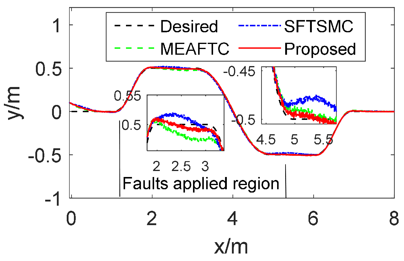
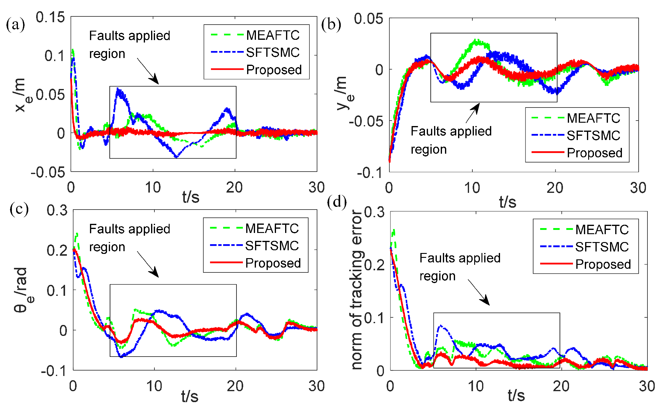
The results of time-varying and constant bias faults, i.e., case 1 and case 2, are presented in this section. In case 1, NMR tracks a random curve, and time-varying LOE and LIP faults are applied during t ( 5 , 20 ) . Figure 5 shows the tracking responses with comparative schemes MEAFTC, SFTSMC and the proposed BF-FOESTSMC. Results indicate that the proposed one is closer to the desired value when faults occur. The tracking errors are presented in Figure 6, the state errors of x e , y e , and θ e in Figure 6a–c show that the proposed FTC scheme has a smaller value, which is more obvious in the Figure 6d of the norm of error given by n o r m ( ς e ) = ( x e 2 + y e 2 + θ e 2 ) . It seems that high-frequency vibrations appear in Figure 6b, this may be influenced by the random external disturbances in the y-direction of the map coordinate, with NMR positioning in a semi-open environment, and then needing frequent control adjustments. Schemes of MEAFTC and SFTSMC have larger tracking error amplitudes when faults occur (the instant t = 5 ) and the average tracking error seems larger under the time-varying faults ( t ( 5 , 20 ) ).
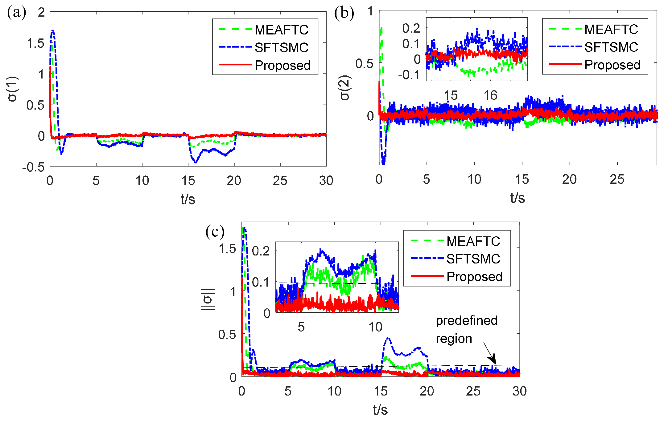
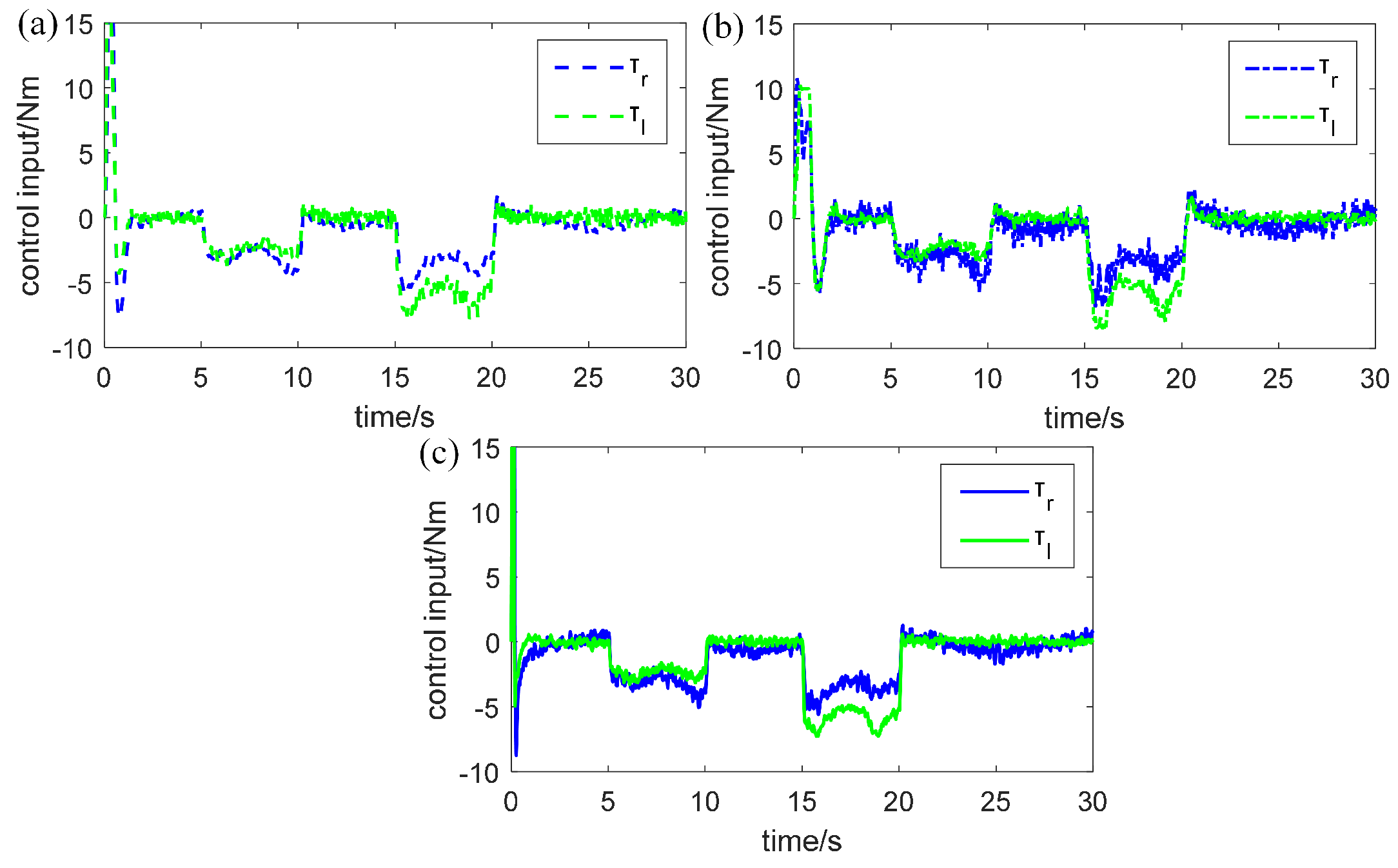
The sliding variables are presented in Figure 7a,b. The SFTSMC achieves convergence in the presence of the faults while large amplitudes are unavoidable and chattering occurs at a steady state. The large amplitudes due to the faults are improved in the MEAFTC method compared with SFTSMC. Under the same circumstances, only the proposed BF-FOESTSMC strategy ensures that the norm of sliding variables | | σ | | can be confined within the predetermined neighborhood of 0.1 under actuator faults and external uncertainty ( t ( 5 , 20 ) ) with less chattering just as Figure 7c presented, which is not discussed in the MEAFTC, SFTSMC (only UUB or asymptotic convergence are guaranteed in their methods). It is noted that in the proposed fault-tolerant controller, the sliding variable converges fast (see the initial time) because the exponential term accelerates the convergence. Figure 8 shows the torque outputs of the compared controller. These results conclude that our strategy is insensitive to time-varying faults and can achieve the predetermined region maintenance even when faults and uncertainties occur.
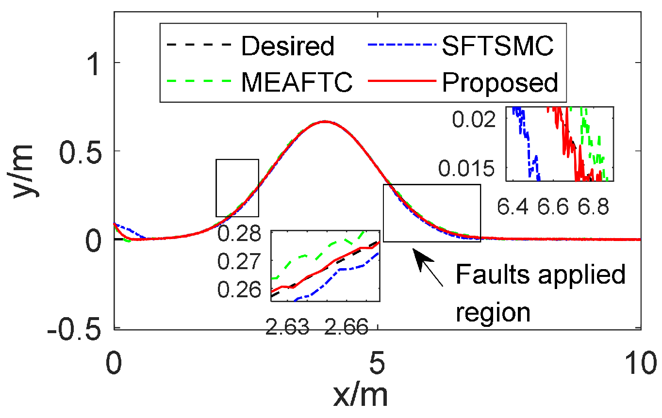
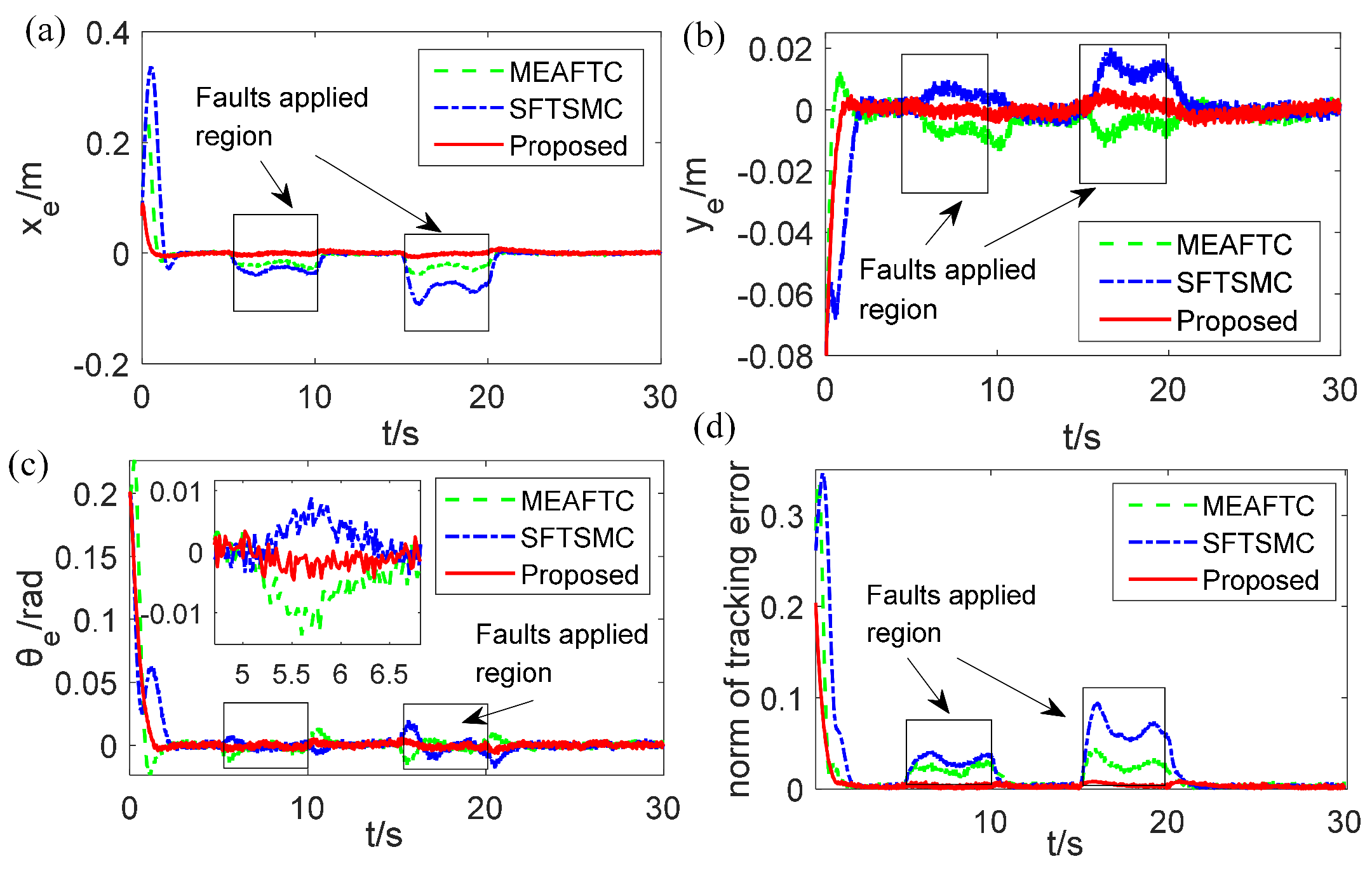
In case 2, NMR follows a Gaussian curve, step LIP failures and random LOE faults (33), are applied when t ( 5 , 10 ) and t ( 15 , 20 ) . From the tracking position response in Figure 9, the proposed method is closer to the expected trajectory under fault conditions under the fault-occurring region. From Figure 10, it seems the MEAFTC and SFTSMC exhibit different levels of amplitude response under time-varying LOE and step-like bias LIP faults, like in x e and y e , and neither can quickly suppress such step faults. Similar to case 1, the high-frequency vibrations presented in Figure 10b may be attributed to the influence of external uncertainties in the y-direction as positioning in a semi-open environment, forcing the control period to adjust to actual location fluctuations. The MEAFTC and SFTSMC have larger errors of θ e when the faults occur or disappear. The n o r m ( ς e ) clearly shows that the proposed controller has smaller norm-tracking errors during t ( 5 , 10 ) and t ( 15 , 20 ) .
From the analysis of the sliding variables in Figure 11, the following conclusions can be drawn: (i) the proposed BF-FOESTSMC reaches the sliding manifold more quickly compared to the other two methods at the initial time, benefiting from the exponential term of the super-twisting sliding mode; (ii) the proposed method is insensitive to the actuator fault due to that the potential barrier function-based adaptive method has sufficient fault suppression capability, which can quickly restore the sliding variables to the origin when the step LIP fault occurs and disappears; (iii) the results in Figure 11c illustrate that the proposed controller can compensate for the LOE and LIP actuator faults, and can guarantee that the sliding variable converges and maintains into the small neighborhood of the origin in a predefined interval 0.1; (iv) the SFTSMC method seems to cause chattering in the steady state. Figure 12 shows the torque outputs of all the controllers.
Table 2 presents the specific indicators of the tracking errors of the two cases in the presence of actuator faults (not including the initial state). Table 3 shows the relative percentages of improvement (RPI) indicators, i.e., relative to the worst case among the three controllers of the norm of dynamic tracking errors | | σ | | . As previously described, case 1 represents two actuators that simultaneously have partial loss effectiveness and time-varying additive inter-turn faults, and case 2 denotes two actuators that simultaneously lose some effectiveness and have unknown drift faults. For a clearer quantitative illustration, the MAX absolute error, RMSE, and MAE are presented. From the results, we can conclude that
(1)
The SFTSMC scheme has the largest MAX errors, which means that it cannot effectively handle the transient errors due to that MAX focuses on the worst-case deviation. In contrast, our proposed controller achieves a great reduction in MAX error in both case 1 and case 2, and the MAX error of | | σ | | is less than 0.1.
(2)
The RMSE indicator shows that the tracking state of our method has much less average deviation in case 1 and case 2 (i.e., time-varying or step-like additive faults), which reflects smoother trajectory tracking, since that RMSE emphasizes larger errors and provides a measure of average performance.
(3)
The MAE of the proposed method can be improved by more than 80% compared to SFTSMC in case 1 and more than 78.2 % in case 2. This indicates that the proposed controller can quickly reduce the error that deviates from the actual values on average, thereby effectively suppressing time-varying LIP or step-like faults.

5. Conclusions

This article investigated a novel adaptive FTC for NMR systems subject to actuator LIP and partial LOE faults. A robust nominal controller was proposed using the exponential super-twisting sliding mode to reduce the reaching phase time. Then, a non-overestimation BF-based gain was proposed to tackle the variation of time-varying LIP faults and uncertainties, while an estimator-based compensation term was designed by estimating the bound of the partial LOE fault coefficients. Combining the nominal controller with BF and LOE fault compensation terms, the adaptive fault-tolerant controller is constructed without requiring the boundary information of faults. The sliding variables achieve fast convergence and are confined in a preset neighborhood in the presence of actuator faults. The results show that the proposed FTC scheme has advantages in fault-tolerant performance compared with other state-of-the-art adaptive FTC approaches, like MEAFTC and SFTSMC schemes.
There is still work to be conducted in our future work. For example, the proposed BF-based gains can theoretically increase to infinity when the fault becomes large, which may not be directly applied to some practical conditions like actuator saturation. We need an anti-saturation method to prevent this problem under the uncertain LOE or LIP faults or find an adaptive law by identifying an error feedback gain to address actuator faults, thereby avoiding the generation of infinite gains. Due to the time-varying uncertainty assumption of the LOE coefficient, the proposed LOE fault compensation term is naturally more complex than the controller design that directly uses a constant boundary value.

Author Contributions

H.W.—investigation, methodology, software, validation, and writing—original draft preparation. S.W.—funding acquisition, conceptualization, resources. Y.X.—supervision, project administration, and writing—review and editing. H.L.—formal analysis, data curation, and writing—review and editing. All authors have read and agreed to the published version of the manuscript.

Funding

The work was funded by National Natural Science Foundation of China under Grant U21A20151, 52105019 and 52305536, China Postdoctoral Science Foundation (2023M731192, 2024T170302), and Guangdong Basic and Applied Basic Research Foundation (2022A1515110880, 2023A1515011650).

Data Availability Statement

Data is contained within the article.

Conflicts of Interest

Author Hu Li was employed by the company Guangdong Intelligent Robotics Institute. The remaining authors declare that the research was conducted in the absence of any commercial or financial relationships that could be construed as a potential conflict of interest.

Abbreviations

ς ,   ς ˙ ,   ς ¨           the state vector of pose, velocity and acceleration of the NMR
( x , y ) , θ           the position, the orientation of NMR
[ x r , y r , θ r ] T , ς e           the desired state vector, the tracking error vector
( x e , y e ) , θ e           position tracking error, the orientation tracking error of NMR
M ( ς ) , C ( ς , ς ˙ )           the symmetric positive definite inertia matrix, centripetal and Coriolis matrix
F ( ς ˙ ) , B ( ς ) , A          surface friction, input transformation matrix, constraints matrix
M ¯ , C ¯ , B ¯ , J           transformation matrix of M, C, B, full rank Jacobian transformation matrix
τ , τ f           the designed controller, the faulty control input
τ f r , τ f l           control inputs of the right motor, control inputs of the left motor

Appendix A

Proof. 
Step 1: Sliding variables reach the ƛ c / 2 -neighborhood of origin in finite time.
Substituting the value of τ n in the model (12), we obtain
υ ˙ = M ¯ 1 ( ς ) B ¯ δ τ C ¯ υ + L 1 ( t ) = ρ D 2 α e ι + υ ˙ ( t ) + μ 1 ( σ ) σ | | σ | | 1 / 2 N ( σ ) ϖ ( t ) + M ¯ 1 B ¯ ( δ 1 ) τ 1 + M ¯ 1 B ¯ δ τ 2 + M ¯ 1 L ( t )
We design the Lyapunov function as
V 1 ( σ ) = 1 2 σ T σ + 1 2 ε 3 ϖ T ϖ +   1 2 δ 0 ˜ T δ ˜ 0
where δ 0 = 1 δ 0 , δ 0 is the low bound of δ , δ ˜ 0 = δ ^ 0 δ 0 . Based on Assumption 2, the time derivative of V 1 ( σ ) is obtained
V ˙ 1 ( σ ) = σ T σ ˙ + 1 ε 3 ϖ T ϖ ˙ +   δ 0 ˜ T δ ˜ ˙ 0 = σ T ( ρ D 2 α e ι + υ ˙ ( t ) υ ˙ ( t ) ) + 1 ε 3 ϖ T ϖ ˙ +   δ 0 ˜ T δ ˜ ˙ 0
Substituting (A1) into (A3) yields
V ˙ 1 ( σ ) = σ T ( μ 1 ( σ ) σ | | σ | | 1 / 2 N ( σ ) + ϖ + M ¯ 1 L ) + σ T M ¯ 1 B ¯ ( 1 δ ) τ 1 σ T M ¯ 1 B ¯ δ 0 δ δ τ 2 + ε 3 ϖ T ϖ ˙ +   δ 0 ˜ T δ ˜ ˙ 0 σ ( μ 1 ( σ ) N 1 ( σ ) | | σ | | 1 / 2 + M ¯ 1 L ) + σ T M ¯ 1 B ¯ δ 0 τ 1 σ T M ¯ 1 B ¯ δ τ 2 +   δ 0 ˜ T δ ˜ ˙ 0
If δ ^ 0 1 δ m , then substituting (24) into (A4), one obtains
V ˙ 1 ( σ ) σ ε 0 t N 1 ( σ ) σ 1 / 2 + M ¯ 1 L m + δ 0 δ ^ 0 1 δ ^ 0 δ m δ σ T M ¯ 1 B ¯ τ 1 + δ 0 ˜ T δ ˜ ˙ 0
Due to that 0 < δ m < δ 0 = 1 δ 0 δ < 1 , we have
V ˙ 1 ( σ ) σ ε 0 t N 1 ( σ ) σ 1 / 2 + M ¯ 1 L m + δ 0 δ ^ 0 δ 0 1 δ ^ 0 σ T M ¯ 1 B ¯ τ 1 +   δ 0 ˜ T δ ˜ ˙ 0 = δ 0 σ ε 0 t N 1 ( σ ) σ 1 / 2 + M ¯ 1 L m + δ ˜ 0 δ ^ ˙ 0 δ ˙ 0 1 1 δ ^ 0 σ T M ¯ 1 B ¯ τ 1
If δ ^ 0 > 1 δ m , combining that 0 < δ m δ 0 < 1 , (A4) can be given as follows by substituting (24) into (A4)
V ˙ 1 ( σ ) σ ε 0 t N 1 ( σ ) σ 1 / 2 + M ¯ 1 L m + δ 0 1 + δ ^ 0 ( 1 δ ^ 0 δ m ) 1 δ ^ 0 δ m δ σ T M ¯ 1 B ¯ τ 1 +   δ 0 ˜ T δ ˜ ˙ 0 σ ε 0 t N 1 ( σ ) σ 1 / 2 + M ¯ 1 L m + δ 0 δ m δ 0 + δ ^ 0 ( 1 δ ^ 0 δ m ) 1 δ ^ 0 σ T M ¯ 1 B ¯ τ 1 +   δ 0 ˜ T δ ˜ ˙ 0 = σ ε 0 t N 1 ( σ ) σ 1 / 2 + M ¯ 1 L m + δ ˜ 0 δ ^ ˙ 0 δ ˙ 0 1 δ m 1 δ ^ 0 σ T M ¯ 1 B ¯ τ 1 +   δ ^ ˙ 0 δ ˜ ˙ 0
Note that δ 0 is the bound of 1 δ , hence δ ˙ 0 = 0 . Substituting (26) into (32) and (33), respectively, the time derivative of V 1 ( σ ) can be expressed as
V ˙ 1 ( σ ) σ ε 0 t N 1 ( σ ) σ 1 / 2 + M ¯ 1 L m
As t is increasing, we can conclude that V ˙ 1 ( σ ) 0 will be satisfied when t > t ¯ = M ¯ 1 L max N 1 ( σ ) / ( ε 0 | | σ | | 1 / 2 ) . σ i ( t ) will decrease in ( t ¯ , t 0 ) , i.e., the super-twisting term can drive the sliding variable scalar | | σ | | to a neighborhood of | | σ | | ƛ c / 2 during t ( t ¯ , t 0 ) . Thus, the sliding variables will reach to the practical sliding manifold s of ƛ c / 2 - neighborhood in finite time. The reachability condition is satisfied. □

Appendix B

Proof. 
Step 2: Sliding variables stay within the predefined ƛ c - neighborhood.
Design the Lyapunov function as
V 2 ( σ ) = 1 2 σ T σ +   1 2 ε 2 ϖ T ϖ + μ ( σ ) +   1 2 δ ˜ 0 T δ ˜ 0
Taking the time derivative of the Lyapunov function (A9), we obtain
V ˙ 2 ( σ ) = σ T ( ρ D 2 α e ι + υ ˙ ( t ) υ ˙ ( t ) ) + 1 ε 2 ϖ T ( μ 2 ( σ ) σ | | σ | | ) + π ƛ c 2 sec 2 π 2 σ T σ ƛ c 2 σ T σ ˙ + δ 0 ˜ T δ ˜ ˙ 0
Substituting (A1) into (A10) yields
V ˙ 2 ( σ ) = σ T μ 1 ( σ ) σ σ 1 / 2 N ( σ ) + ϖ ( t ) + M ¯ 1 L ( t ) + 1 ε 2 ϖ T μ 2 ( σ ) σ σ + σ T π ƛ c 2 sec 2 π 2 σ T σ ƛ c 2 μ 1 ( σ ) σ σ 1 / 2 N ( σ ) + ϖ + σ T M ¯ 1 B ¯ ( 1 δ ) τ 1 σ T M ¯ 1 B ¯ δ τ 2 + δ 0 ˜ T δ ˜ ˙ 0
and V ˙ ( σ ) can be simplified as follows
V ˙ 2 ( σ ) = μ 1 ( σ ) σ T σ σ 1 / 2 N ( σ ) + σ T ϖ ( t ) + σ T M ¯ 1 L ( t ) π ƛ c 2 sec 2 π 2 σ T σ ƛ c 2 μ 1 ( σ ) σ T σ σ 1 / 2 N ( σ ) + σ T M ¯ 1 B ¯ ( 1 δ ) τ 1 σ T M ¯ 1 B ¯ δ τ 2 + δ 0 ˜ T δ ˜ ˙ 0 σ ( μ 1 ( σ ) N 1 ( σ ) σ 1 / 2 + ϖ ( t ) + M ¯ 1 L m ) + σ T M ¯ 1 B ¯ ( 1 δ ) τ 1 σ T M ¯ 1 B ¯ δ τ 2 + δ 0 ˜ T δ ˜ ˙ 0
If δ ^ 0 1 δ m , then substituting (24) into (A12), one obtains
V ˙ 2 ( σ ) σ ( μ 1 ( σ ) N 1 ( σ ) σ 1 / 2 + Δ ) + δ 0 δ ^ 0 1 δ ^ 0 δ m δ σ T M ¯ 1 B ¯ τ 1 + δ 0 ˜ T δ ˜ ˙ 0
where Δ = Δ ϖ ( t ) + M ¯ 1 L m . Similar to (A5) and (A6), (A13) can be rewritten as
V ˙ 2 ( σ ) σ ( μ 1 ( σ ) N 1 ( σ ) σ 1 / 2 + Δ ) + δ ˜ 0 δ ^ ˙ 0 δ ˙ 0 1 1 δ ^ 0 σ T M ¯ 1 B ¯ τ 1
If δ ^ 0 > 1 δ m , similar to (A7) and (A8), we have
V ˙ 2 ( σ ) σ μ 1 ( σ ) N 1 ( σ ) σ 1 / 2 + Δ + δ ˜ 0 δ ^ ˙ 0 δ ˙ 0 1 δ m 1 δ ^ 0 σ T M ¯ 1 B ¯ τ 1 + δ 0 ˜ T δ ˜ ˙ 0
Substituting (26) into (A14) and (A15), respectively, the time derivative of V 2 ( σ ) can be expressed as
V ˙ 2 ( σ ) σ μ 1 ( σ ) N 1 ( σ ) σ 1 / 2 + Δ
Due to that μ 1 ( σ ) = ε 1 ƛ c 2 π tan π 2 σ T σ ƛ c 2 , obviously, μ 1 ( σ ) is monotonically increasing when | | σ | | approaches ƛ c and ψ ( σ ) will be negative as | | σ | | ƛ c . To find the solution of ψ ( σ ) = 0 , we have the following approximation:
lim | | σ | | ƛ c tan π 2 σ T σ ƛ c 2 = lim | | s | | ƛ c tan π 2 π 2 · ƛ c 2 σ T σ ƛ c 2 = lim | | s | | ƛ c 1 sin π 2 · ƛ c 2 σ T σ ƛ c 2 = lim | | s | | ƛ c 2 π ƛ c 2 ƛ c 2 σ T σ
Substituting (A17) into (A13) yields
V ˙ 2 ( σ ) σ 2 ε 1 π ƛ c 2 N 1 ( σ ) ƛ c 2 σ T σ | | σ ( t ) | | 1 / 2 + Δ = 2 ε 1 π Δ N 1 ( σ ) ƛ c 2 σ T σ ƛ c 2 Δ N 1 ( σ ) | | σ ( t ) | | 1 / 2 ƛ c 2 + | | σ ( t ) | | 2 σ
If σ satisfies the following
σ σ ¯ , ƛ c ,
where σ ¯ = max ƛ c 2 ƛ c 2 / ( Δ N 1 ( σ ) ) 2 / 3 , 0 , then Δ > 0 , hence V ˙ 2 ( σ ) 0 . This means V ( σ ) is negative when σ ¯ σ < ƛ c , and the error variable will force σ decrease to σ σ ¯ < ƛ c . This proves the convergence of the variables on t > 0 . In the case of t t 0 , the variable gain is switched to the barrier function and the sliding variable meets σ < ƛ c . When the unknown LIP fault grows, the BF-based gain will increase and σ will never leave the ƛ c -neighborhood of zero. This completes the proof. □

References

  1. Jiang, L.; Wang, S.; Xie, Y.; Xie, S.; Zheng, S.; Meng, J.; Ding, H. Decoupled fractional supertwisting stabilization of interconnected mobile robot under harsh terrain conditions. IEEE Trans. Ind. Electron. 2022, 69, 8178–8189. [Google Scholar] [CrossRef]
  2. Ao, W.; Zhang, L.; Zhang, H.; Li, Z.; Huang, G. Structure design and event-triggered control of a modular omnidirectional mobile chassis of life support robotics. Fractal Fract. 2023, 7, 121. [Google Scholar] [CrossRef]
  3. Gupta, M.; Kumar, S.; Behera, L.; Subramanian, V.K. A novel vision-based tracking algorithm for a human-following mobile robot. IEEE Trans. Syst. Man Cybern. Syst. 2017, 47, 1415–1427. [Google Scholar] [CrossRef]
  4. Labbadi, M.; Boubaker, S.; Djemai, M.; Mekni, S.K.; Bekrar, A. Fixed-time fractional-order global sliding mode control for nonholonomic mobile robot systems under external disturbances. Fractal Fract. 2022, 6, 177. [Google Scholar] [CrossRef]
  5. Jia, F.; Huang, J.; He, X. Predefined-time fault-tolerant control for a class of nonlinear systems with actuator faults and unknown mismatched disturbances. IEEE Trans. Autom. Sci. Eng. 2024, 21, 3801–3815. [Google Scholar] [CrossRef]
  6. Kamel, M.; Yu, X.; Zhang, Y. Fault-tolerant cooperative control design of multiple wheeled mobile robots. IEEE Trans. Control Syst. Technol. 2018, 26, 756–764. [Google Scholar] [CrossRef]
  7. Van, M.; Ge, S.S.; Ren, H. Finite time fault tolerant control for robot manipulators using time delay estimation and continuous nonsingular fast terminal sliding mode control. IEEE Trans. Cybern. 2016, 47, 1681–1693. [Google Scholar] [CrossRef]
  8. Guo, B.; Chen, Y. Robust adaptive fault-tolerant control of fourwheel independently actuated electric vehicles. IEEE Trans. Ind. Informat. 2020, 16, 2882–2894. [Google Scholar] [CrossRef]
  9. Zhang, G.; Liu, S.; Zhang, X. Adaptive distributed fault-tolerant control for underactuated surface vehicles with bridge-to-bridge event-triggered mechanism. Ocean Eng. 2022, 262, 112205. [Google Scholar] [CrossRef]
  10. Wu, F.; Liu, Y.; Fang, Y.; Liu, L.; Lei, Z. Fault estimation and active fault-tolerant control for a class of nonlinear systems with actuator and sensor faults based on unknown input iterative learning. Asian J. Control 2024, 26, 376–392. [Google Scholar] [CrossRef]
  11. Zhang, X.; Xu, X.; Li, J.; Ma, F.; Zhang, Z.; Brunauer, G.; Steyskal, F. Fault estimation and H∞ fuzzy active fault-tolerant control design for ship steering autopilot subject to actuator and sensor faults. IEEE Sens. J. 2023, 23, 28110–28119. [Google Scholar] [CrossRef]
  12. Gao, Z.; Zhang, Y.; Guo, G. Finite-time fault-tolerant prescribed performance control of connected vehicles with actuator saturation. IEEE Trans. Veh. Technol. 2022, 72, 1438–1448. [Google Scholar] [CrossRef]
  13. Wu, K.; Hu, J.; Ding, Z.; Arvin, F. Finite-time fault-tolerant formation control for distributed multi-vehicle networks with bearing measurements. IEEE Trans. Autom. Sci. Eng. 2023, 21, 1346–1357. [Google Scholar] [CrossRef]
  14. Gong, J.; Jiang, B.; Ma, Y.; Mao, Z. Distributed adaptive fault-tolerant formation—Containment control with prescribed performance for heterogeneous multiagent systems. IEEE Trans. Cybern. 2022, 53, 7787–7799. [Google Scholar] [CrossRef] [PubMed]
  15. Li, P.; Yang, G. Backstepping adaptive fuzzy control of uncertain nonlinear systems against actuator faults. J. Control Theory Appl. 2009, 7, 248–256. [Google Scholar] [CrossRef]
  16. Xiao, B.; Hu, Q.; Shi, P. Attitude stabilization of spacecraft under actuator saturation and partial loss of control effectiveness. IEEE Trans. Control Syst. Technol. 2013, 21, 2251–2263. [Google Scholar] [CrossRef]
  17. Zhang, X.; Xie, Y.; Jiang, L.; Li, G.; Meng, J.; Huang, Y. Fault-tolerant dynamic control of a four-wheel redundantly-actuated mobile robot. IEEE Access 2019, 7, 157909–157921. [Google Scholar] [CrossRef]
  18. Singh, P.; Nandanwar, A.; Behera, L.; Verma, N.K.; Nahavandi, S. Uncertainty compensator and fault estimator-based exponential supertwisting sliding-mode controller for a mobile robot. IEEE Trans. Cybern. 2021, 52, 11963–11976. [Google Scholar] [CrossRef]
  19. Ijaz, S.; Galea, M.; Hamayun, M.T.; Ijaz, H.; Javaid, U. A new output integral sliding mode fault-tolerant control and fault estimation scheme for uncertain systems. IEEE Trans. Autom. Sci. Eng. 2024, 21, 4214–4225. [Google Scholar] [CrossRef]
  20. Rotondo, D.; Puig, V.; Nejjari, F.; Romera, J. A fault-hiding approach for the switching quasi-LPV fault-tolerant control of a four-wheeled omnidirectional mobile robot. IEEE Trans. Ind. Electron. 2014, 62, 3932–3944. [Google Scholar] [CrossRef]
  21. Yang, H.; Yin, S.; Kaynak, O. Neural network-based adaptive fault-tolerant control for Markovian jump systems with nonlinearity and actuator faults. IEEE Trans. Syst., Man, Cybern., Syst. 2020, 51, 3687–3698. [Google Scholar] [CrossRef]
  22. Diao, S.; Sun, W.; Su, S.F.; Xia, J. Adaptive fuzzy event-triggered control for single-link flexible-joint robots with actuator failures. IEEE Trans. Cybern. 2021, 52, 7231–7241. [Google Scholar] [CrossRef] [PubMed]
  23. Argha, A.; Su, S.W.; Celler, B.G. Static output feedback fault tolerant control using control allocation scheme. Int. J. Robust Nonlinear Control 2019, 29, 98–116. [Google Scholar] [CrossRef]
  24. Qin, M.; Dian, S.; Guo, B. Fractional-order SMC controller for mobile robot trajectory tracking under actuator fault. Syst. Sci. Control Eng. 2022, 10, 312–324. [Google Scholar] [CrossRef]
  25. Ma, Y.; Jiang, B.; Cocquempot, V. Modeling and adaptive fault compensation for two physically linked 2WD mobile robots. IEEE/ASME Trans. Mech. 2021, 26, 1161–1171. [Google Scholar] [CrossRef]
  26. Ma, Y.; Cocquempot, V.; El Najjar, M.E.; Jiang, B. Adaptive compensation of multiple actuator faults for two physically linked 2WD robots. IEEE Trans. Robot. 2017, 34, 248–255. [Google Scholar] [CrossRef]
  27. Shen, Z.; Ma, Y.; Song, Y. Robust adaptive fault-tolerant control of mobile robots with varying center of mass. IEEE Trans. Ind. Electron. 2017, 65, 2419–2428. [Google Scholar] [CrossRef]
  28. Xiao, B.; Cao, L.; Xu, S.; Liu, L. Robust tracking control of robot manipulators with actuator faults and joint velocity measurement uncertainty. IEEE/ASME Trans. Mech. 2020, 25, 1354–1365. [Google Scholar] [CrossRef]
  29. Deng, Y.; Wang, J.; Li, H.; Liu, J.; Tian, D. Adaptive sliding mode current control with sliding mode disturbance observer for PMSM drives. ISA Trans. 2019, 88, 113–126. [Google Scholar] [CrossRef]
  30. Song, Z.; Liu, J.; Liu, Y.; Hu, Y.; Fang, F. Fault-tolerant control of floating wind turbine with switched adaptive sliding mode controller. IEEE Trans. Autom. Sci. Eng. 2024, 21, 3705–3718. [Google Scholar] [CrossRef]
  31. Relaño, C.; Muñoz, J.; Monje, C.A.; Martínez, S.; González, D. Modeling and control of a soft robotic arm based on a fractional order control approach. Fractal Fract. 2022, 7, 8. [Google Scholar] [CrossRef]
  32. Xie, Y.; Zhang, X.; Meng, W.; Zheng, S.; Jiang, L.; Meng, J.; Wang, S. Coupled fractional-order sliding mode control and obstacle avoidance of a four-wheeled steerable mobile robot. ISA Trans. 2021, 108, 282–294. [Google Scholar] [CrossRef] [PubMed]
  33. Fallaha, C.J.; Saad, M.; Kanaan, H.Y.; Al-Haddad, K. Sliding-mode robot control with exponential reaching law. IEEE Trans. Ind. Electron. 2010, 58, 600–610. [Google Scholar] [CrossRef]
  34. Saied, H.; Chemori, A.; Bouri, M.; Rafei, M.E.; Francis, C. Feedforward super-twisting sliding mode control for robotic manipulators: Application to PKMs. IEEE Trans. Robot. 2023, 39, 3167–3184. [Google Scholar] [CrossRef]
  35. Obeid, H.; Laghrouche, S.; Fridman, L.; Chitour, Y.; Harmouche, M. Barrier function-based adaptive super-twisting controller. IEEE Trans. Autom. Control 2020, 65, 4928–4933. [Google Scholar] [CrossRef]
  36. Mendoza-Avila, J.J.; Moreno, A.; Fridman, L.M. Continuous Twisting Algorithm for Third-Order Systems. IEEE Trans. Autom. Control 2020, 65, 2814–2825. [Google Scholar] [CrossRef]
  37. Xie, Y.; Tang, X.; Song, B.; Zhou, X.; Guo, Y. Data-driven adaptive fractional order PI control for PMSM servo system with measurement noise and data dropouts. ISA Trans. 2018, 75, 172–188. [Google Scholar] [CrossRef]
  38. Obeid, H.; Fridman, L.M.; Laghrouche, S.; Harmouche, M. Barrier function-based adaptive sliding mode control. Automatica 2018, 93, 540–544. [Google Scholar] [CrossRef]
  39. Chen, J.; Wu, C.; Yu, G.; Narang, D.; Wang, Y. Path following of wheeled mobile robots using online-optimization-based guidance vector field. IEEE/ASME Trans. Mech. 2021, 26, 1737–1744. [Google Scholar] [CrossRef]
  40. Fierro, R.; Lewis, F.L. Control of a nonholonomic mobile robot using neural networks. IEEE Trans. Neural Netw. 1998, 9, 589–600. [Google Scholar] [CrossRef]
  41. Li, J.W. Adaptive tracking and stabilization of nonholonomic mobile robots with input saturation. IEEE Trans. Autom. Control 2021, 67, 6173–6179. [Google Scholar] [CrossRef]
  42. Nagesh, I.; Edwards, C. A multivariable super-twisting sliding mode approach. Automatica 2014, 50, 984–988. [Google Scholar] [CrossRef]
  43. Chen, Z.; Liu, Y.; He, W.; Qiao, H.; Ji, H. Adaptive-neural-network-based trajectory tracking control for a nonholonomic wheeled mobile robot with velocity constraints. IEEE Trans. Ind. Electron. 2021, 68, 5057–5067. [Google Scholar] [CrossRef]
  44. Wu, H.; Wang, S.; Xie, Y.; Li, H.; Zheng, S.; Jiang, L. Adaptive abrupt disturbance rejection tracking control for wheeled mobile robots. IEEE Robot. Autom. Lett. 2024, 9, 7787–7794. [Google Scholar] [CrossRef]
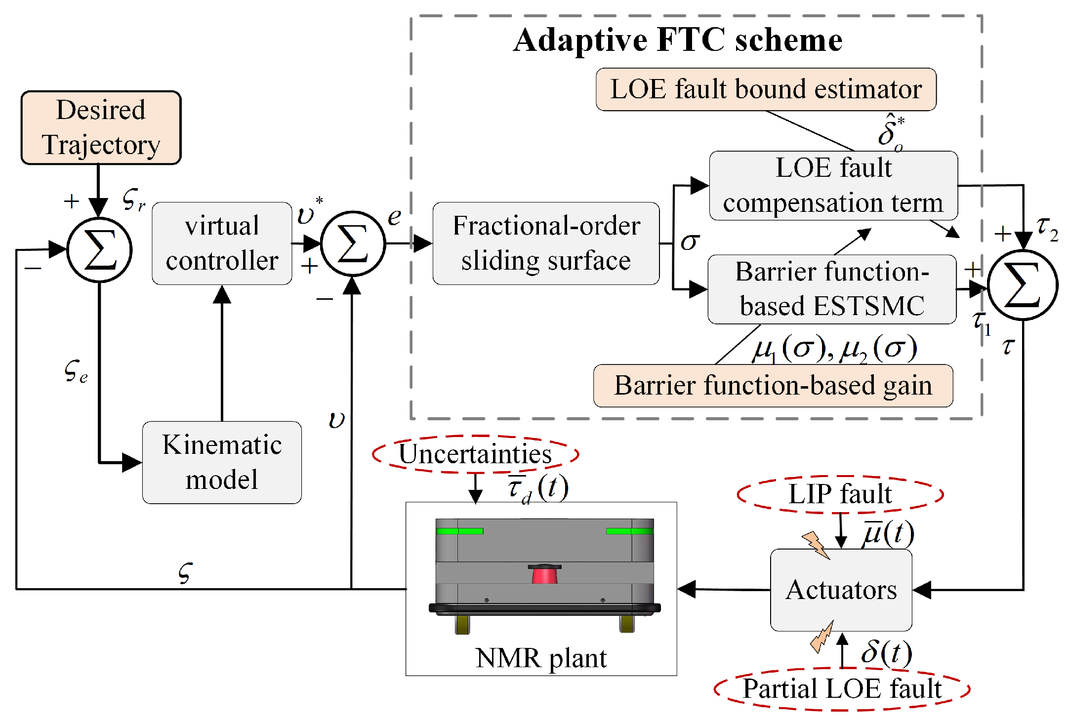
Figure 1. Overall control framework of the proposed adaptive FTC scheme.
Fractalfract 08 00612 g001
Figure 2. The prototype of the developed NMR.
Fractalfract 08 00612 g002
Figure 3. Hardware architecture of the developed NMR.
Fractalfract 08 00612 g003
Figure 4. The implementation procedure of the proposed CFSMC BF-FOESTSMC scheme.
Fractalfract 08 00612 g004
Figure 5. Case 1: Position tracking performance of compared schemes and the proposed FTC.
Fractalfract 08 00612 g005
Figure 6. Case 1: State tracking errors. (a) x e . (b) y e . (c) θ e . (d) n o r m ( ς e ) .
Fractalfract 08 00612 g006
Figure 7. Case 1: Sliding variables. (a) σ ( 1 ) . (b) σ ( 2 ) . (c) | | σ | | .
Fractalfract 08 00612 g007
Figure 8. Case 1: Control outputs. (a) MESFTC. (b) SFTSMC. (c) proposed controller.
Fractalfract 08 00612 g008
Figure 9. Case 2: Position tracking performance of compared schemes and the proposed FTC.
Fractalfract 08 00612 g009
Figure 10. Case 2: State tracking errors. (a) x e . (b) y e . (c) θ e . (d) n o r m ( ς e ) .
Fractalfract 08 00612 g010
Figure 11. Case 2: Sliding variables. (a) σ ( 1 ) . (b) σ ( 2 ) . (c) | | σ | | .
Fractalfract 08 00612 g011
Figure 12. Case 2: Control outputs. (a) MESFTC. (b) SFTSMC. (c) proposed controller.
Fractalfract 08 00612 g012
Table 1. Parameters of the NMR.
ParametersValuesParametersValues
Max speed1.5 m/sRobot length0.8 m
RAM of PC8 GRobot width 2 b 0.52 m
Encoder2500 pprTotal mass m80 kg
Laser sweep distance30 mWheel diameter 2 r 0.16 m
Table 2. Error indicators of the schemes under actuator faults.
SignalsErrorsSchemesMAX ( 10 3 )RMSE ( 10 3 )MAE ( 10 3 )
case 1: simultaneously
partial LOE and time-
varying LIP faults
x e MEAFTC26.19.97.4
SFTSMC55.716.111.6
Proposed7.32.01.6
y e MEAFTC29.711.18.6
SFTSMC25.310.08.5
Proposed12.55.54.8
θ e MEAFTC52.421.817.5
SFTSMC68.926.921.7
Proposed31.613.210.7
| | σ | | MEAFTC230.447.362.1
SFTSMC496.494.5122.4
Proposed81.415.831.5
case 2: simultaneously
partial LOE and unknown
bias LIP faults
x e MEAFTC42.311.710.3
SFTSMC92.726.020.0
Proposed9.12.82.1
y e MEAFTC14.33.53.9
SFTSMC20.15.54.5
Proposed6.62.11.6
θ e MEAFTC15.63.92.8
SFTSMC21.04.53.0
Proposed6.41.81.5
| | σ | | MEAFTC238.553.162.2
SFTSMC456.8107.7117.7
Proposed75.215.425.6
Table 3. RPI indicators of | | σ | | .
SFTSMCMEAFTCProposed
MAX of | | σ | | in case 10%53.6%83.6%
RMSE of | | σ | | in case 10%49.9%83.3%
MAE of | | σ | | in case 10%49.3%74.3%
MAX of | | σ | | in case 20%47.8%83.5%
RMSE of | | σ | | in case 20%50.7%85.7%
MAE of | | σ | | in case 20%47.2%78.2%
Disclaimer/Publisher’s Note: The statements, opinions and data contained in all publications are solely those of the individual author(s) and contributor(s) and not of MDPI and/or the editor(s). MDPI and/or the editor(s) disclaim responsibility for any injury to people or property resulting from any ideas, methods, instructions or products referred to in the content.