Article

A Fractional-Order Model Predictive Control Strategy with Takagi–Sugeno Fuzzy Optimization for Vehicle Active Suspension System

1
School of Mechatronics and Vehicle Engineering, East China Jiaotong University, Nanchang 330013, China
2
Key Laboratory of Vehicle Intelligent Equipment and Control of Nanchang City, East China Jiaotong University, Nanchang 330013, China
3
Vehicle Performance and Testing Department, Jiangling Motor Corporation Limited Company, Nanchang 330200, China
*
Author to whom correspondence should be addressed.
Fractal Fract. 2024, 8(10), 610; https://doi.org/10.3390/fractalfract8100610
Submission received: 16 September 2024 / Revised: 11 October 2024 / Accepted: 15 October 2024 / Published: 18 October 2024

Abstract

:
Aiming at the problem of system controller performance failure caused by improperly setting the value of each weighting coefficient of the model predictive control (MPC), a fractional-order MPC strategy with Takagi–Sugeno fuzzy optimization (T–SFO MPC) is proposed for a vehicle active suspension system. Firstly, the fractional-order model predictive control framework for active suspension systems is designed based on a 1/4 vehicle model. Then, we analyze the influence of different weighting coefficients on the suspension performance and introduce the Takagi–Sugeno fuzzy optimization theory to adaptively adjust the weighting coefficients of the fractional-order MPC controller. Finally, the system responses of the T–SFO MPC, traditional MPC, linear quadratic regulator (LQR), and passive suspension control are numerically analyzed under various road conditions. Simulation results show that suspension response with the T–SFO MPC is significantly improved compared with passive suspension control, traditional MPC control, and LQR control, and the weight coefficients of the T–SFO MPC can be adaptively adjusted according to the dynamic changes of suspension response. Compared with passive suspension, the root mean square (RMS) value of the vertical acceleration of the T–SFO MPC under various roads decreased by a maximum of 37.97%, and the RMS value of suspension dynamic deflection and tire dynamic load decreased by a maximum of 32.94% and 37.8%, respectively. These results validate that the proposed control method can achieve coordinated optimization of vehicle comfort and handling stability.

1. Introduction

The vehicle suspension system transmits the forces and torques acting between the wheels and the body, which effectively dampens vibrations caused by uneven road surfaces [1,2]. In the technological development of vehicle suspension systems, suspension control methods mainly include passive control, semi-active, and active control [3], and the application of advanced control theories to active suspension systems is generally recognized as one of the effective ways to improve suspension performance. The active suspension control method attenuates vehicle vibration by generating active force through the actuating device, which can achieve optimal control effect and has been widely used in various vehicle vibration control applications [4].
At present, many scholars in this field have carried out in-depth research on the design of active suspension system controllers, such as optimal control, sliding mode control, and reinforcement learning control, to realize the goal of improving vehicle comfort and handling stability of suspension systems [5]. Zhao et al. proposed a sliding model control strategy based on a linear quadratic regulator, which uses a proportional integral sliding mode controller to track the reference force and calculates the reference force in real time by the linear quadratic regulator and force command planner [6]. Bai et al. designed a robust optimal integral sliding mode control strategy based on the initial optimal controller, which can achieve the optimal control objective and has good robustness to uncertain parameters and external disturbances [7]. Liu et al. proposed a robust integral terminal sliding mode control method, which can enable the system to converge quickly in a finite time far from the equilibrium point and reduce the jitter phenomenon in traditional sliding mode control [8]. Wang et al. proposed a control method that integrates deep reinforcement learning while considering system characteristics, using an action delay mechanism and hard constraint module to solve time delay and actuator dynamic constraint problems, thus verifying that the method can effectively alleviate vehicle body vibration in the low-frequency range [9]. Lee et al. designed a deep reinforcement learning controller that selected a built-in algorithm adapted to suspension in deep reinforcement learning to improve the convergence of training, thus verifying the optimal performance of the controller in terms of ride comfort [10]. Although these intelligent control algorithms have achieved significant results in the field of suspension control, it is difficult to effectively handle some issues, such as multivariate constraints, high real-time requirements, and model uncertainty.
Model predictive control (MPC) is a control strategy widely used in vehicle control technology for addressing multi-variate constraints in the rolling time domain. MPC strategies commonly used in the field of vehicle suspension can be mainly divided into traditional MPC, distributed model predictive control (DMPC), nonlinear model predictive control (NMPC), and explicit model predictive control (EMPC). Papadimitrakis et al. proposed a road foresight MPC based on a radial basis function (RBF) model, which effectively approximates the nonlinear behavior of the suspension system, thus improving the performance of the linear MPC [11]. Zhang et al. proposed a fast DMPC method based on multiple intelligences, which utilizes the RBF neural network to solve the partial differential equations of rolling optimization, thereby improving the computational efficiency of the algorithm [12]. Ricco et al. proposed two new real-time implicit NMPC formulas, the first based on a pseudoinverse decoupling transformation for obtaining the damping force contributions and the second using an inverse formulation to verify that the adaptable NMPC configuration has the best performance in all simulation scenarios [13]. Li et al. proposed an EMPC based on road preview, which transforms the control problem based on rolling optimization into an explicit polyhedral system and improves the computational efficiency of the control system through offline pre-calculation of control state relationships [14]. In recent years, a new type of fractional order model predictive control has attracted attention. Yaghini et al. designed a linear time-varying fractional order model predictive control method and verified that the proposed method has significantly stable performance when faced with multiple input constraints [15].
Although traditional MPC can effectively handle various variable constraints, it still has certain limitations in dealing with changes in road conditions and complex models. In this regard, some control methods have integrated the idea of variable time domain and variable weights into the MPC control framework. The selection of these parameters needs to be debugged and optimized according to the actual system [16]. Zhang et al. proposed a novel path-tracking model predictive control strategy with Laguerre functions and exponential weights, introducing a fitted orthogonal sequence composed of Laguerre functions to reduce the massive optimization control parameters of MPC with longer control ranges [17]. Batta et al. defined four interference curves, step, dual mode, the third mock examination, and ISO8608 D-type curves, as the weight basis of the MPC process to optimize each configuration file, which verified the effectiveness of MPC in reducing the driver’s absorption power based on the multi-mode active suspension concept [18]. Sun et al. proposed a model predictive thrust control method applied to the evaluation function of linear motors, which uses the evaluation function to select the optimal voltage vector and applies it to the next control cycle to achieve faster speed dynamic response [19]. Dogruer et al. proposed a fast-constrained model predictive control algorithm with orthogonal Laguerre polynomials and used Laguerre polynomials to prove that the optimization parameter set can be minimized, thus verifying that online optimization takes less time [20].
However, these papers only optimize the intrinsic parameters of MPC without considering the stability of the controller and whether the variable weights are suitable for the quality of the system response. If the controller objective can adaptively adjust to changes in various road conditions, then the optimal system response can be obtained. Accordingly, this paper proposes a fractional-order MPC strategy of active suspension based on T–S fuzzy variable weight. First, a 1/4 vehicle active suspension system model with two degrees of freedom is established in Section 2.1; the fractional-order model predictive control framework for active suspension system is designed in Section 2.2 and Section 2.3 to reduce steady-state errors and enhance the stability of the controller. Second, to adaptively adjust the weights of each control quantity in the controller according to different road conditions, a fractional-order MPC strategy with Takagi–Sugeno fuzzy optimization (T–SFO MPC) is proposed to achieve adaptive optimization of the weights in Section 3. Finally, simulation analysis is carried out on random terrain and bumpy roads to verify the proposed T–SFO MPC in Section 4.

2. Design of a Fractional-Order MPC Controller for Active Suspension

2.1. Dynamics Modeling for Active Suspension

To obtain the actual driving condition of the vehicle suspension, a 1/4 vehicle active suspension model with two degrees of freedom is adopted directly [21,22], as shown in Figure 1. According to existing modeling methods, the differential equation of motion for the 1/4 vehicle suspension model is derived based on Newton’s second theorem, as shown in Equation (1).
m b z ¨ b + k s z b z w + c s z ˙ b z ˙ w u = 0                                                       m w z ¨ w + k t z w z r k s z b z w c s z ˙ b z ˙ w + u = 0 .
where m b   and   m w are the spring-loaded mass and unsprung mass of the vehicle, respectively; k s , k t   and c s   are the suspension stiffness, tire stiffness, and suspension damping coefficient, respectively; z b   and z w are the body and wheel displacements, respectively; z r   is the displacement of road excitation; u   is the input control force for the vehicle suspension system.
The input control force u of the vehicle suspension is taken as the input vector of the system, and the system state vector Z and output vector Y are chosen as follows:
Z = [ z ˙ b z ˙ w         z b z w z w z r ] T Y = [ z ¨ b z b z w         z w z r ] T                   .
Then, the state space equation of the system model can be expressed as follows:
Z ˙ = A Z + B U + F W Y = C Z + D U                         .
where A is the input matrix of the state vector; B is the input matrix for the control force; F is the input matrix for the road excitation; C is the output matrix of the state vector; D is the output matrix of the control force; U is the input vector of the control force; W is the input vector of road excitation.
Among them, the following is true:
A = c s m b c s m b         c s m w c s m w         k s m b 0         k s m w k t m w 1         1 0                 1           0           0     0             0         , B = 1 m b 1 m w 0 0 T
C = c s m b 0 0 c s m b 0 0 k s m b 0         1     0           0     1   , D = 1 m b 0 0 T
F = 0 0 0 1 T ,   U = u , W = z ˙ r

2.2. Predictive Model of MPC

The principle of the MPC control algorithm of active suspension is shown in Figure 2. It mainly consists of a discretized predictive model of active suspension, fractional control objective function, and working constraints. The state equations obtained from Equation (3) are continuous and cannot be used directly for MPC controller design. Therefore, the approximate discretization of the system state space model using the forward Euler method can be expressed as follows:
Z ˙ Z k + 1 Z k / T .
where T denotes the sampling period. Then the discretized state space equation can be expressed as follows:
Z ( k + 1 ) = A ~ Z ( k ) + B ~ U ( k ) + F ~ W ( k ) Y b ( k ) = C ~ b Z ( k ) + D ~ b U ( k ) Y c ( k ) = C ~ c Z ( k )                                                                                     .
where A ~ = I + T A ,   B ~ = T B , F ~ = T F , and I is the unit matrix of the corresponding dimension; Z ( k ) R n z is the state quantity at time moment k; U ( k ) R n u is the control input quantity at time moment k; W ( k ) R n w is the road disturbance at time moment k; Y b ( k ) R n b is the control output quantity; Y c ( k ) R n c is the constraint output quantity. The output matrix and feedforward matrix of the discrete state space model are consistent with the continuous time state space model.
The MPC strategy can deal with optimization problems with constraints in a finite time domain. Taking the latest measurements of the system as the initial condition, define the prediction step size and control step size as N p and N c , respectively, where N c N p . Based on the linear discrete-time state space Equation (5) of the 1/4 vehicle suspension model and the latest measured state quantity Z(k), the control increment U(k), and the road disturbance W(k) is derived in N p iterations to obtain the predicted state quantities and control outputs for the N p steps. After optimizing the MPC controller and obtaining the control input for step N c , the first control input is applied to the suspension discrete system, and the system performs control progress [23]. Define the sequence of predicted output quantities Y ^ ( k ) , the sequence of predicted state quantities Z(k), the control input quantities U(k), and the sequence of predicted external input perturbations W(k) for the system from the k-moment to the future Np-steps, respectively, as follows:
Y ^ k Y b k + 1 k Y b k + 2 k Y b k + N p k T .
Z k Z k + 1 k Z k + 2 k Z k + N p k T .
U k U k + 1 k U k + 2 k U k + N c k T .
W k W k k W k + 1 k W k + N p 1 k T .
Then, the output state equation of the active suspension model for the future N p steps at time moment k within the control step is as follows:
Y ^ k = A ^ Z k + B ^ U k + F ^ W k .
where
A ^ = C ~ b A ~ C ~ b A ~ 2 C ~ b A ~ N p N p × 1 T
B ^ = C ~ b B ~ C ~ b A ~ B ~                 D ~ b C ~ b B ~ 0 0                                                         C ~ b A ~ N p 1 B ~ C ~ b A ~ N p 2 B ~ D ~ b + i = 1 N p N c C ~ b A ~ i 1 B ~ N p × ( N c + 1 )
F ^ = C ~ b F ~ C ~ b A ~ F ~                 0 C ~ b F ~ 0 0                                                         C ~ b A ~ N p 1 F ~ C ~ b A ~ N p 2 F ~ C ~ b F ~ N p × N p

2.3. Fractional Objective Function of MPC

The MPC controller needs to make the system output error close to the reference output while satisfying the constraints of the suspension system. The response values of the suspension system, z ¨ b , z b z w , and   z w z r , should track the reference values as closely as possible. Moreover, during the roll optimization process, the control quantity U(k) and the road disturbance W(k) will have some interference with the system output value, so the input force of the active suspension should not be changed too fast to avoid overshooting of the controller. To solve the problem of interference in the system output values, incremental control of the system inputs is introduced and used as a cost in the performance metrics to generate smoother control inputs. In order to reduce steady-state errors and enhance the stability of the controller, this paper effectively combines the principle of the Grünwald–Letnikov fractional order integral with the objective function of model predictive control. When the state and output quantities of the system are given, the incremental values of the system reference output and system control input are defined as Y ^ r e f k = A ^ Z r e f k + F ^ W k , U k = U k U k 1 , respectively, then the fractional order objective function of MPC is shown in Equation (11).
J = Φ T N p T α Q [ Y ^ ( k ) Y ^ r e f ( k ) ] 2 + Φ T N c T β R u U ( k ) 2 + Φ T N c T β R u U ( k ) 2               = T N p T ψ 1 α Q Y ^ k Y ^ r e f k 2 d t + T N c T ψ 1 β ( R u U ( k ) 2 + R u U ( k ) 2 ) d t .
Q = d i a g Q 1 , Q 2 , , Q N c , , Q N p ,       Q i = d i a g q 1 , q 2 , q 3 , i = 1,2 , , N p .
R u = d i a g R 0 , R 1 , R 2 , , R N c 1 , R j = [ q u ] , j = 1,2 , , N c 1 .
R u = d i a g R 0 , R 1 , R 2 , , R N c 1 , R n = [ q u ] , n = 1,2 , , N c 1 .
where Q is the error weight matrix between the predicted output and the reference output; R u is the weight matrix of the controller control input; R u is the weight matrix of the controller input incremental; Φ and ψ are the fractional order integral and derivative notation, respectively; α and β denote the order of fractional-order integrals; q 1 is the weight of vertical acceleration; q 2 is the weight of suspension dynamic deflection; q 3 is the weight of tire dynamic deformation; q u is the weight of control input; q u is the weight of control input incremental.
Then, the fractional objective function of Equation (11) can be discretized using the method described in [24,25] as follows:
J F O Q Г ( T , α 1 ) [ Y ^ ( k ) Y ^ r e f ( k ) ] 2 + R u Г ( T , α 2 ) U ( k ) 2 + R u Г ( T , α 2 ) U ( k ) 2 Q ¯ Y ^ k Y ^ r e f k 2 + R u ¯ U k 2 + R u ¯ U k 2                                                                               .
where
Q ¯ = Q Г ( T , α 1 ) ,   R u ¯ = R u Г ( T , α 2 ) ,   R u ¯ = R u Г T , α 2 .
Г T , α 1 = T α 1 d i a g ( X N p , X N p 1 , , X 1 , X 0 ) ,   Г T , α 2 = T α 2 d i a g X N C , X N C 1 , , X 1 , X 0 .
with X i = ω i α j ω ( i H + 1 ) α j , S = N p for j = 1, S = N C for j = 2 and ω i α j can be obtained as follows:
ω i α j = 1 1 α j i ω i α j 1       i > 0 1                                                                     i = 0 0                                                                     i < 0 .
The quadratic programming problem is the key to solving the MPC optimization problem, so the objective Function (15) needs to be rewritten in standard quadratic form. Define the reference state Z r e f ( k ) at moment k; then, the system output error is as follows:
Y ^ k Y ^ r e f k = A ^ Z k A ^ Z r e f k + B ^ U k .
The fractional objective function can be rewritten as follows:
J F O U f k T H U f k + E ^ k T Q ¯ E ^ k + 2 G T U f k .
where E ^ ( k ) A ^ Z ( k ) A ^ Z r e f ( k ) , U f ( k ) U ( k ) U ( k ) T , H = d i a g B ^ T Q ¯ B ^ + R u ¯ , R u ¯ , and G T = E ^ ( k ) T Q ¯ B ^ 0 . The second term, E ^ k T Q ¯ E ^ k , is determined by the state quantity of the system and is not affected by the control quantity U f k . Therefore, the controller can ignore it in the optimization calculation to obtain the new objective function as follows:
J F O U f k T H U f k + 2 G T U f k .
The MPC controller can handle constraints explicitly, and its closed-loop optimization problems need to consider multiple constraint settings. There exist thresholds for the control force inputs to the controller of the vehicle active suspension, which are defined to be U m a x and U m i n . Then, the controller inputs are constrained to be as follows:
U m i n U k + i k U m a x , i = 1,2 , , N c .
Due to the limitation of the mechanical structure, the dynamic deflection of the suspension should be constrained within the range of the working stroke to avoid the damper hitting the limit block. The maximum working stroke of the damper can be defined as Y s w s .
z b z w Y s w s .
To ensure the driving safety and maneuvering stability of the vehicle, it is necessary to ensure effective contact between the tires and the ground, and the dynamic load of the tires should be less than the static load of the vehicle, to reduce the impact of the wheels and the road surface, i.e., the following:
k t ( z w z r ) m b + m w g .
Therefore, the controller output constraint should be satisfied:
Y m i n Y c k + i k Y m a x , i = 1,2 , , N p .
The optimization problem of the MPC objective function under multiple constraints can be described as a quadratic optimal programming problem that solves for the optimal value, which can be expressed while satisfying the system constraints as follows:
J O F U ( k ) m i n U f k T H U f k + 2 G T U f k .                                               s . t .   U m i n U k + i k U m a x , i = 1,2 , , N c .               Y m i n Y c k + i k Y m a x ,   i = 1,2 , , N p .

3. Fractional-Order MPC Strategy with Takagi–Sugeno Fuzzy Optimization

Compared with the traditional Mamdani fuzzy control, T–S fuzzy control is more suitable for dealing with complex nonlinear systems. Its output is a clear value or a linear function related to the input quantity, which can be directly applied to the controller and has the advantages of faster operation speed and more accurate control [26,27,28]. Therefore, to enhance the adaptive capability of working conditions during vehicle driving, the T–S fuzzy method is adopted to adaptively optimize the weights of fractional order MPC.

3.1. The Effect of Different Weights on Suspension Performance

Before designing the T–S fuzzy controller, the effect of MPC weighting coefficients on suspension performance needs to be considered. For the 1/4 vehicle suspension, the vertical acceleration, suspension dynamic deflection, and tire dynamic deformation are usually considered as evaluation indicators for the vibration characteristics of the vehicle suspension. Therefore, these three performance indicators are set in Equation (2) for output observation and used to analyze the impact of different weights on suspension performance.
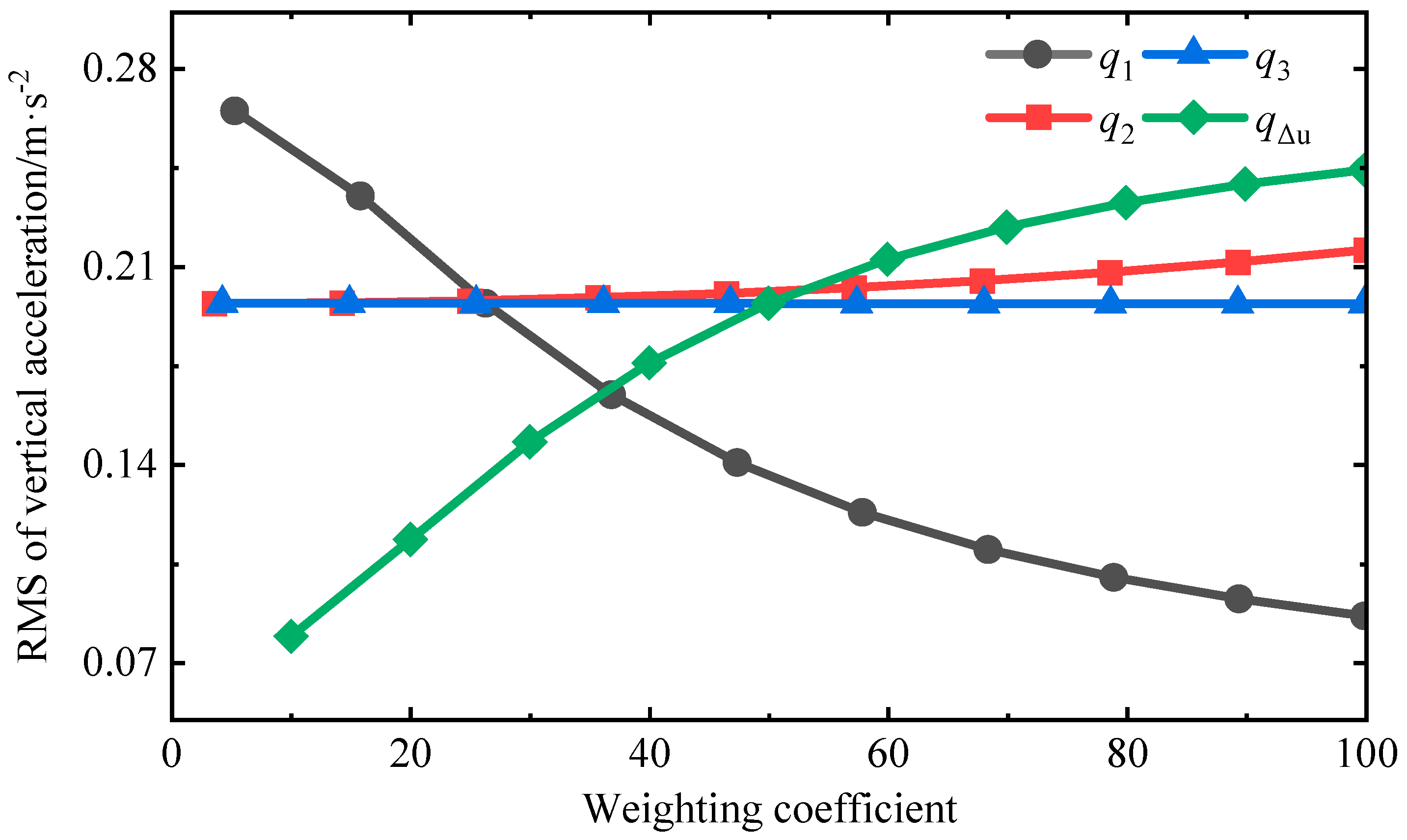
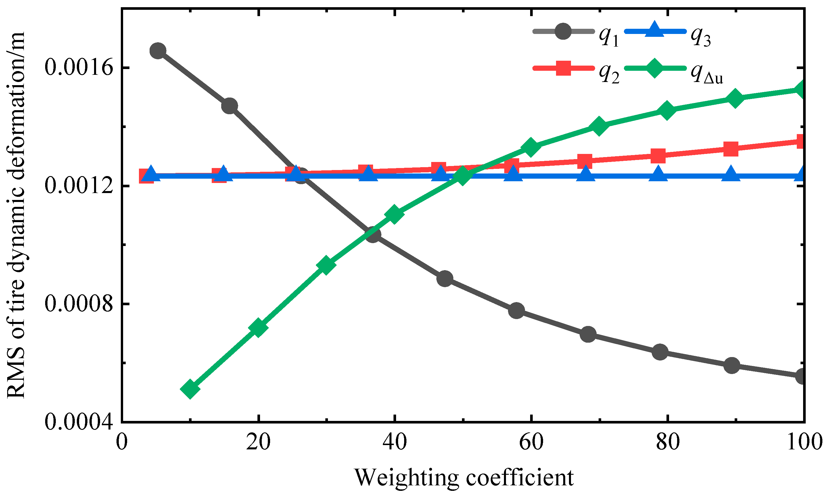
Combining Equations (1)–(26), the simulation of the active suspension system can be executed. From Equations (11)–(14), the weighting coefficients affecting the suspension comfort are q 1 , q 2 , q 3 , q u and q u , which act on the vertical acceleration, suspension dynamic deflection, tire dynamic deformation, control input, and control input incremental, respectively. By analyzing the performance of the vehicle suspension system with different weighting coefficients acting under the same operating conditions, the weighting coefficients are coordinated to realize the optimal control of the controller, which provides the key design guidance for the T–S fuzzy rule table. This paper uses a single control variable method to study the impact of different weighting coefficients on suspension performance. The adjustable range of each weighting coefficient in the simulation progress is shown in Table 1. The suspension vibration simulation is conducted by controlling one of the weighting coefficients to vary in a specified increment while keeping the remaining weighting coefficients constant. In the control scenario, the initial constants for each weighting coefficient are q 1 = 50 , q 2 = 50 , q 3 = 60 , q u = 0.01 , and q u = 1.5. By calculating the root mean square (RMS) values of suspension performance under different weight coefficients, the effect of different weighting coefficients on suspension performance is shown in Figure 3, Figure 4 and Figure 5, and the values of each weight coefficient are uniformly scaled within the horizontal coordinate range.
As can be seen from Figure 3, Figure 4 and Figure 5, the RMS values of vertical acceleration and tire dynamic deformation rapidly decrease with the increase in q 1 , while the RMS value of suspension dynamic deflection shows a slow changing trend of first decreasing and then increasing. Although a larger q 1 can make the vertical acceleration and tire dynamic deformation improved greatly, the optimization effect of the vehicle suspension dynamic deflection has been greatly reduced. The reason is that a larger q 1 is not sensitive to improving the suspension dynamic deflection, while a smaller q 1 cannot effectively improve the vertical acceleration and tire dynamic deformation. Therefore, only changing q 1 cannot satisfy the requirement of vehicle suspension to improve comfort and needs to be coordinated with other weighting coefficients. If the weighting coefficient q 2 is too large, there is a gradual increase in the three performance indicators at this time, and this will cause a significant decrease in the performance of the controller. When q 2 is small, the three performance indicators have been greatly reduced, and the controller control effect has been improved to some extent. Therefore, it is necessary to control q 2 in a small range to avoid a performance deterioration in the control effect of the controller. Smaller weighting coefficients q u can lead to significant improvements in the vertical acceleration and tire dynamic deformation, but the optimal range of control input increment for suspension dynamic deflection is within a relatively small weight range. Too large a q u will result in poor control performance. Therefore, it needs to be controlled within an appropriate weight range to adjust the control effect on the three performance indexes.

3.2. Establishment of Takagi–Sugeno Fuzzy Optimization

From the above analysis results, it can be seen that the control system is susceptible to vertical acceleration and suspension dynamic deflection. So, the vertical acceleration tracking error e ( z ¨ b ) and the suspension dynamic deflection tracking error e ( z b z w ) are set as the fuzzy control inputs in the T–S fuzzy optimization, and the fuzzy outputs in the T–S fuzzy optimization are the values of q 1 , q 2 , q 3 , and q u . The domain of the T–S fuzzy input variable e ( z ¨ b ) is set to [−1.2, 1.2] and the domain of the input domain e ( z b z w ) is set to [−0.085, 0.085]. The fuzzy subsets of the input variables are set to five, which are {VL (negative large), L (negative small), M (medium), H (positive small), and VH (positive large)}, and the triangular affiliation function is used for both input variables. In the T–S fuzzy optimization theory, the fuzzy inputs and the output variables have a linear relationship, and the relationship can be described as follows:
R i : I f     e ( z ¨ b ) = A i   a n d     e ( z b z w ) = A i t h e n   y = p                                                                                   .
where R i is the ith fuzzy rule, i = 1,2 , , n ; y is the ith output variable; p is the corresponding fuzzy value; A i is a certain fuzzy subset of the ith fuzzy rule.
The T–S fuzzy rules are detailed in Table 2, Table 3, Table 4 and Table 5. The domains of fuzzy controller output variables p q 1 , p q 2 , p q 3 , and p q u are set to [0, 1], and the following equation expresses the relationship between the different weighting coefficients and fuzzy control output variables.
q 1 = p q 1 q 1 g a i n           q 2 = p q 2 q 2 g a i n                 q 3 = p q 3 q 3 g a i n                 q u = p q u q u g a i n .
where q 1 g a i n = 50 ,   q 2 g a i n = 50 , q 3 g a i n = 60 , and q u g a i n = 1.5 .

3.3. Design of T–SFO MPC

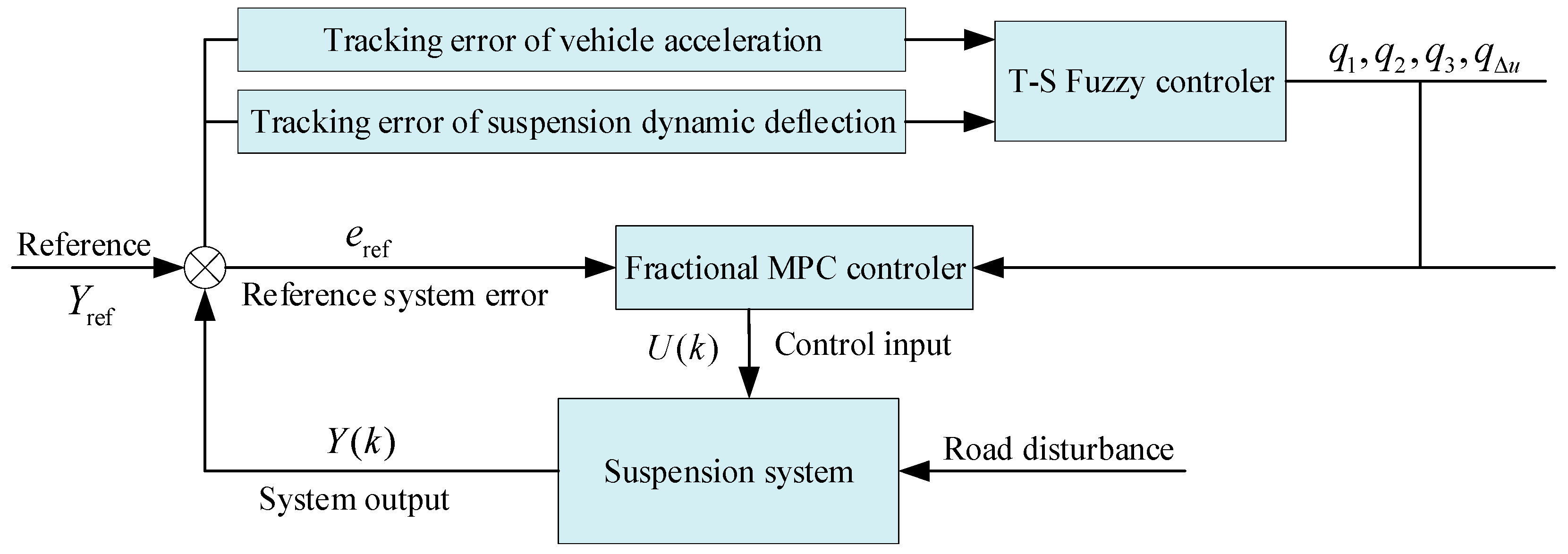
By designing the fuzzy optimization rules, the relationship between the fuzzy outputs of the controller and the performance indicators of vehicle suspension can be determined. When the vertical acceleration and tire dynamic deformation are reduced, q 1 can be appropriately reduced, while   q 2 , q 3 , and q u can be appropriately increased. When the vertical acceleration, suspension dynamic deflection, and tire dynamic deformation are increased, q 1   can be appropriately increased, while   q 2 , q 3 , and q u can be appropriately reduced. So, the establishment of T–S fuzzy variable-weight adaptive control with comfort, maneuvering stability, and adaptability, and its control structure, are shown in Figure 6.

4. Simulation Result

To verify the effectiveness of the T–SFO MPC control strategy, the vehicle suspension system is analyzed by numerical simulation. After manual debugging based on previous work experience [2], the selected parameters of the vehicle suspension system are used in Section 2.1 and Section 2.2, as shown in Table 6. The selected MPC controller parameters are used in Section 2.3, as shown in Table 7.
Firstly, two different road excitations are established as an input state for the simulation scenarios of the suspension system. Then, to compare the control effect, passive suspension without control input in Section 2.1 is applied, the traditional MPC strategy in Section 2.3 and the T–SFO MPC strategy in Section 3 are used to control the active suspension system, and the controlled suspension response can be obtained. Finally, the vertical acceleration z ¨ b , suspension dynamic deflection z b z w , and tire dynamic load k t ( z w z r ) are taken as the output state and evaluation indexes of the suspension response. The suspension responses under passive suspension control, traditional MPC control, linear quadratic regulator (LQR) control, and T–SFO MPC control are compared and analyzed.

4.1. Random Terrain Road

Random terrain road using Gaussian white noise to simulate the road excitation, setting the white noise power as 1, the sampling time as 0.005 s, and the road unevenness coefficient as 6.4 × 10⁻⁵ m3. The simulation can be obtained as the random terrain road excitation, as shown in Figure 7.
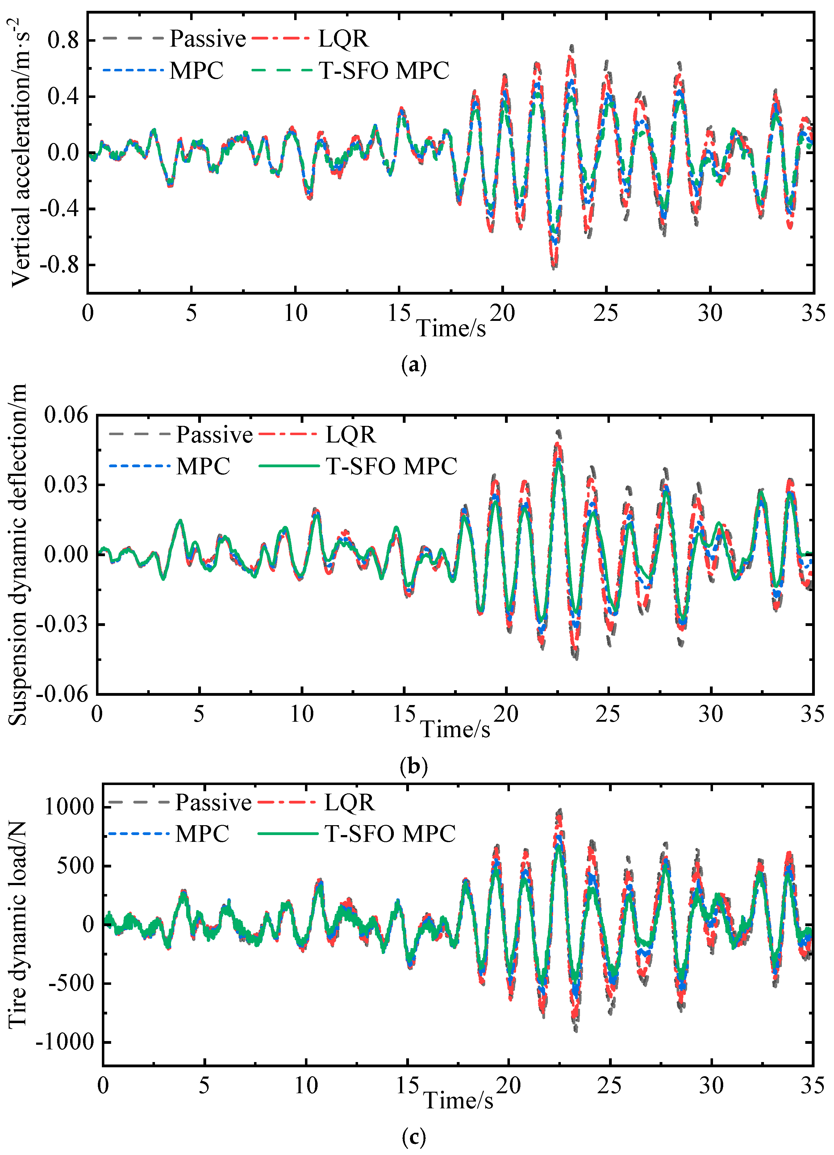
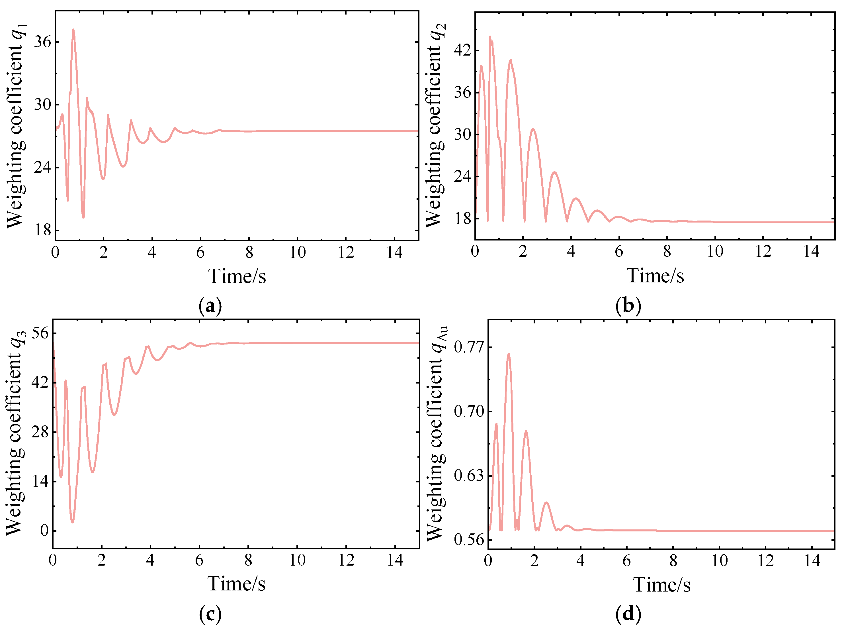
Simulation results of four different control strategies on the response of suspension systems under random terrain are shown in Figure 8, and the variation curves of four weighting coefficients using the T–S fuzzy optimization strategy are shown in Figure 9. The RMS values of vertical acceleration, suspension dynamic deflection, and tire dynamic load for the vehicle suspension system with four different control strategies are shown in Table 8.
As shown in Figure 8, the peak values of vertical acceleration, suspension dynamic deflection, and tire dynamic load under the T–SFO MPC control are lower than those of the other control strategies. Meanwhile, it can be seen that the T–SFO MPC control is more adaptive compared to other controls when the vehicle is traveling on random terrain. Therefore, the active suspension under the T–SFO MPC control can effectively suppress the body sagging vibration caused by the road surface unevenness and mitigate the high-frequency impact of the suspension system on the body sagging upward. Moreover, compared with the traditional MPC control, the T–SFO MPC control can effectively reduce the suspension dynamic deflection while ensuring comfort is not affected, avoiding excessive amplitude that may cause the vehicle to roll and sway. In addition, as shown in Figure 9, it can be seen that each weight coefficient increases in the later stage compared to the previous stage. The weight coefficient adjustment of suspension performance is significantly higher than that of control variable weight coefficients, thus achieving the optimal suspension performance. This proves that the proposed control strategy can automatically adjust weight coefficients based on suspension response to adapt to deteriorating vehicle performance. As shown in Table 8, compared with the passive suspension, the RMS values of vertical acceleration, suspension dynamic deflection, and tire dynamic load are reduced by 37.97%, 32.94%, and 37.80%, respectively, for the suspension system under the T–SFO MPC control. Compared with the traditional MPC control, the RMS values of vertical acceleration, suspension dynamic deflection, and tire dynamic load of the suspension system are also reduced by 14.54%, 10.24%, and 14.43%, respectively. Therefore, under the excitation of random terrain road, the control effect of the T–SFO MPC control strategy can significantly improve the vehicle ride’s comfort and ensure the vehicle’s maneuvering stability.

4.2. Bump Road

To further verify the adaptive performance of the T–SFO MPC control, a bump road is set on a section of smooth road, and the mathematical model of the bump road is established with a sinusoidal function, which is expressed as follows:
z r = H 1 2 ( 1 cos 2 π v 1 L 1 t ) , 0 t L 1 v 1 0 ,                                                                                     t L 1 v 1 .
where H 1 is the bump road height, H 1 = 0.07 m; v 1 is the speed of the vehicle traveling on the bumpy road, v 1 = 20 km/h; L 1 is the length of the bumpy pavement, and L 1 = 0.8 m. The bump road input excitation obtained from the simulation is shown in Figure 10.
Simulation results of four different control strategies on the response of suspension systems under bumpy road are shown in Figure 11, and the variations of each weighting coefficient under the T–S fuzzy optimization strategy are shown in Figure 12. The RMS values of vertical acceleration, suspension dynamic deflection, and tire dynamic load for the vehicle suspension under four different control strategies are shown in Table 9.
As shown in Figure 11, when the vehicle passes through the bumpy road, all the response peaks of the active suspension under the three control strategies are effectively suppressed, among which the oscillations under the T–SFO MPC control are the fastest to decay, and its vibration-damping effect is better than the remaining three control strategies. As shown in Figure 12, when driving on a bumpy road, the weight coefficients are continuously adaptively adjusted, and, when driving on a flat road, they begin to become stable. As shown in Table 9, the suspension system under the T–SFO MPC control reduces the vertical acceleration, suspension dynamic deflection, and tire dynamic load by 30.20%, 25.00%, and 30.49%, respectively, compared to the passive suspension. The RMS values of vertical acceleration, suspension dynamic deflection, and tire dynamic load of the suspension system are reduced by 12.34%, 7.55%, and 12.49%, respectively, as compared to the traditional MPC control. These processes demonstrate that weight coefficients can be effectively optimized by the T–S fuzzy strategy. Therefore, under the excitation of bumpy road, the control effect of the T–SFO MPC control strategy can significantly improve the vehicle ride’s comfort and ensure the vehicle’s maneuvering stability.

5. Conclusions

Aiming at addressing the comfort and maneuvering stability of vehicle suspension systems under multiple road conditions, this paper proposes a T–SFO MPC control strategy for active suspension systems. The effects of different weighting coefficients on the performance of the vehicle active suspension system are analyzed by modeling a 1/4 vehicle active suspension system. Then, the effectiveness of the T–SFO MPC control strategy in improving vehicle comfort in a variety of road conditions is verified by the simulation results.
The proposed T–SFO MPC control strategy can adaptively adjust different weighting coefficients under a variety of road conditions, which is better than passive control, traditional MPC control, and LQR control in terms of comfort and stability. Compared to passive suspension control under random terrain and bump road conditions, the RMS values of the vertical acceleration of the T–SFO MPC decreased by 37.97% and 30.20%, respectively, the RMS values of the suspension dynamic deflection of the T–SFO MPC decreased by 32.94% and 25%, respectively, and the RMS values of the tire dynamic load of the T–SFO MPC decreased by 37.8% and 30.49%, respectively. Therefore, the proposed T–SFO MPC control performs well under a variety of road conditions with strong adaptability. These results validate that the proposed control method can achieve coordinated optimization of vehicle comfort and handling stability.

Author Contributions

Writing—original draft preparation, Q.L.; conceptualization, B.H.; methodology, J.L.; validation, W.L.; formal analysis, W.Y.; writing—review and editing, G.H.; project administration, G.L. All authors have read and agreed to the published version of the manuscript.

Funding

This research was funded by the National Natural Science Foundation of China (No. 52405104), Natural Science Foundation Project of Jiangxi Province (20242BAB20249 and 20232BAB204041), Key R&D project of Jiangxi Province of China (No. 20212BBE51009), Key Program for International S&T Cooperation Project of Jiangxi Province of China (20232BBH80010), Jiangxi Graduate Student Innovation Special Fund Project (YC2023-S463 and YC2024-S426), and Double Height Project of Jiangxi Province Human Resources and Social Security Department in 2022.

Data Availability Statement

Data are contained within the article.

Conflicts of Interest

Author Wei Liu was employed by the Jiangling Motor Corporation Limited Company. The remaining authors declare that the research was conducted in the absence of any commercial or financial relationships that could be construed as potential conflicts of interest.

References

  1. Soliman, A.M.A.; Kaldas, M.M.S. Semi-active suspension systems from research to mass-market—A review. J. Low Freq. Noise Vib. Act. Control 2021, 40, 1005–1023. [Google Scholar] [CrossRef]
  2. Liu, Q.J.; Chen, W.; Hu, H.S.; Hu, G.L.; Zhu, Q.Y. Effect of magnetorheological damper parameters on dynamic responses of a full-vehicle suspension system. Int. J. Appl. Electromagn. Mech. 2020, 63, 483–503. [Google Scholar] [CrossRef]
  3. Theunissen, J.; Tota, A.; Gruber, P.; Dhaens, M.; Sorniotti, A. Preview-based techniques for vehicle suspension control: A state-of-the-art review. Annu. Rev. Control 2021, 51, 206–235. [Google Scholar] [CrossRef]
  4. Rana, R.S.; Dipak, M.A. Two-degree of freedom-based control model for active suspension system to mitigate the nonlinear disturbance. J. Circuits Syst. Comput. 2023, 32, 2350312. [Google Scholar] [CrossRef]
  5. Al-Ashmori, M.; Wang, X. A systematic literature review of various control techniques for active seat suspension systems. Appl. Sci. 2020, 10, 1148. [Google Scholar] [CrossRef]
  6. Zhao, Z.K.; Wang, C.W.; Zhao, J.Q.; Du, W. LQR force command planning–based sliding mode control for active suspension system. Proc. Inst. Mech. Eng. Part I J. Syst. Control Eng. 2024, 238, 373–385. [Google Scholar] [CrossRef]
  7. Bai, R.; Wang, H.B. Robust optimal control for the vehicle suspension system with uncertainties. IEEE Trans. Cybern. 2021, 52, 9263–9273. [Google Scholar] [CrossRef]
  8. Liu, Y.J.; Chen, H. Adaptive sliding mode control for uncertain active suspension systems with prescribed performance. IEEE Trans. Syst. Man Cybern. Syst. 2020, 51, 6414–6422. [Google Scholar] [CrossRef]
  9. Wang, C.; Cui, X.X.; Zhao, S.J.; Zhou, X.R.; Song, Y.Q.; Wang, Y.; Guo, K.H. Enhancing vehicle ride comfort through deep reinforcement learning with expert-guided soft-hard constraints and system characteristic considerations. Adv. Eng. Inform. 2024, 59, 102328. [Google Scholar] [CrossRef]
  10. Lee, D.; Jin, S.; Lee, C. Deep reinforcement learning of semi-active suspension controller for vehicle ride comfort. IEEE Trans. Veh. Technol. 2022, 72, 327–339. [Google Scholar] [CrossRef]
  11. Papadimitrakis, M.; Alexandridis, A. Active vehicle suspension control using road preview model predictive control and radial basis function networks. Appl. Soft Comput. 2022, 120, 108646. [Google Scholar] [CrossRef]
  12. Zhang, N.N.; Yang, S.; Wu, G.Y.; Ding, H.T.; Zhang, Z.; Guo, K.H. Fast distributed model predictive control method for active suspension systems. Sensors 2023, 23, 3357. [Google Scholar] [CrossRef] [PubMed]
  13. Ricco, M.; Alshawi, A.; Gruber, P.; Dhaens, M.; Sorniotti, A. Nonlinear model predictive control for yaw rate and body motion control through semi-active and active suspensions. Veh. Syst. Dyn. 2024, 62, 1587–1620. [Google Scholar] [CrossRef]
  14. Li, W.; Liang, H.J.; Xia, D.B.; Fu, J.; Yu, M. Explicit model predictive control of magnetorheological suspension for all-terrain vehicles with road preview. Smart Mater. Struct. 2024, 33, 035037. [Google Scholar] [CrossRef]
  15. Yaghini, H.H.; Kharrati, H.; Rahimi, A. Linear time-varying fractional-order model predictive attitude control for satellite using two reaction wheels. Aerosp. Sci. Technol. 2024, 145, 108901. [Google Scholar] [CrossRef]
  16. Yang, T.; Li, P.; Li, Q.; Li, Z. Active suspension control strategy for vehicles based on road surface recognition. Nonlinear Dyn. 2024, 112, 11043–11065. [Google Scholar] [CrossRef]
  17. Zhang, B.; Zong, C.; Chen, G.; Zhang, B. Electrical vehicle path tracking based model predictive control with a Laguerre function and exponential weight. IEEE Access 2019, 7, 17082–17097. [Google Scholar] [CrossRef]
  18. Batta, N.A.; Daniel, P.D. Model predictive control of a multi-mode suspension system using preview information and weight optimization. J. Dyn. Syst. Meas. Control 2023, 145, 065001. [Google Scholar] [CrossRef]
  19. Sun, X.; Wu, M.; Yin, C.; Wang, S. Model predictive thrust force control for linear motor actuator used in active suspension. IEEE Trans. Energy Convers. 2021, 36, 3063–3072. [Google Scholar] [CrossRef]
  20. Dogruer, C.U. Constrained model predictive control of a vehicle suspension using Laguerre polynomials. Proc. Inst. Mech. Eng. Part C J. Mech. Eng. Sci. 2020, 234, 1253–1268. [Google Scholar] [CrossRef]
  21. Hsiao, C.Y.; Wang, Y.H. Evaluation of ride comfort for active suspension system based on self-tuning fuzzy sliding mode control. Int. J. Control Autom. Syst. 2022, 20, 1131–1141. [Google Scholar] [CrossRef]
  22. Dehghan, M.; Fateh, M.M.; Ghalehnoie, M. A fuzzy-supervised impedance control for an active suspension system. J. Vib. Eng. Technol. 2023, 11, 3257–3266. [Google Scholar] [CrossRef]
  23. Kim, J.; Lee, T.; Kim, C.J.; Yi, K. Model predictive control of a semi-active suspension with a shift delay compensation using preview road information. Control Eng. Pract. 2023, 137, 105584. [Google Scholar] [CrossRef]
  24. Mohanty, D.; Panda, S. Modified salp swarm algorithm-optimized fractional-order adaptive fuzzy PID controller for frequency regulation of hybrid power system with electric vehicle. J. Control Autom. Electr. Syst. 2021, 32, 416–438. [Google Scholar] [CrossRef]
  25. Safari, A.; Yaghini, H.H.; Kharrati, H.; Rahimi, A.; Oshnoei, A. Voltage controller design for offshore wind turbines: A machine learning-based fractional-order model predictive method. Fractal Fract. 2024, 8, 463. [Google Scholar] [CrossRef]
  26. Vassilyev, S.N.; Kudinov, Y.I.; Pashchenko, F.F.; Durgaryan, I.S.; Kelina, A.Y.; Kudinov, I.Y.; Pashchenko, A.F. Intelligent control systems and fuzzy controllers. II. trained fuzzy controllers, fuzzy PID controllers. Autom. Remote Control 2020, 81, 922–934. [Google Scholar] [CrossRef]
  27. Yuan, Q.; Zhou, H.L.; Chen, S.L.; Miao, W.W.; Jiang, Y.F. Designing a Switched Takagi-Sugeno Fuzzy controller for CDC semi-active suspensions with current input constraint. Mech. Syst. Signal Process. 2023, 199, 110450. [Google Scholar]
  28. Shi, J.Z.; Huang, W.W.; Zhou, Y. T–S fuzzy control of travelling-wave ultrasonic motor. J. Control Autom. Electr. Syst. 2020, 31, 319–328. [Google Scholar]
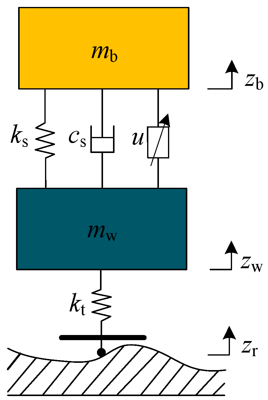
Figure 1. The 1/4 vehicle suspension system model.
Fractalfract 08 00610 g001
Figure 2. MPC control framework of active suspension.
Fractalfract 08 00610 g002
Figure 3. RMS value of vertical acceleration under different weighting coefficients.
Fractalfract 08 00610 g003
Figure 4. RMS value of suspension dynamic deflection under different weighting coefficients.
Fractalfract 08 00610 g004
Figure 5. RMS value of tire dynamic deformation under different weighting coefficients.
Fractalfract 08 00610 g005
Figure 6. Design of T–SFO MPC.
Fractalfract 08 00610 g006
Figure 7. Random terrain road.
Fractalfract 08 00610 g007
Figure 8. Vehicle suspension response under random terrain. (a) Vertical acceleration; (b) suspension dynamic deflection; (c) tire dynamic load.
Fractalfract 08 00610 g008
Figure 9. Variation curves of weighting coefficients under random terrain. (a) q 1 ; (b)   q 2 ; (c) q 3 ; (d) q u .
Fractalfract 08 00610 g009
Figure 10. Bump road.
Fractalfract 08 00610 g010
Figure 11. Vehicle suspension response under bump road. (a) Vertical acceleration; (b) suspension dynamic deflection; (c) tire dynamic load.
Fractalfract 08 00610 g011
Figure 12. Variation curves of weighting coefficients under bump road. (a) q 1 ; (b)   q 2 ; (c) q 3 ; (d) q u .
Fractalfract 08 00610 g012
Table 1. Adjustable range for each weighting coefficient.
ParameterValue
The weight of vertical acceleration q 1 10:20:190
The weight of suspension dynamic deflection q 2 50:150:1400
The weight of tire dynamic deformation q 3 10:25:235
The weight of control input q u 0.01
The weight of control input incremental q u 0.3:0.3:3
Table 2. Fuzzy rule for output variable p q 1 .
e ( z b z w ) e ( z ¨ b )
VLLMHVH
VL0.660.550.280.550.66
L0.850.550.280.550.85
M0.980.660.550.660.98
H0.850.550.280.550.85
VH0.660.550.280.550.66
Table 3. Fuzzy rule for output variable p q 2 .
e ( z b z w ) e ( z ¨ b )
VLLMHVH
VL0.750.350.230.350.75
L0.940.750.350.750.94
M0.940.940.350.940.94
H0.940.750.350.750.94
VH0.750.350.230.350.75
Table 4. Fuzzy rule for output variable p q 3 .
e ( z b z w ) e ( z ¨ b )
VLLMHVH
VL00.250.530.250
L00.250.530.250
M0.250.530.890.530.25
H00.250.530.250
VH00.250.530.250
Table 5. Fuzzy rule for output variable p q u .
e ( z b z w ) e ( z ¨ b )
VLLMHVH
VL0.580.580.40.580.58
L0.40.40.30.40.4
M0.40.30.30.30.4
H0.40.40.30.40.4
VH0.580.580.40.580.58
Table 6. Vehicle suspension parameter.
ParameterValue
Spring loaded mass m b /(kg)390
Unsprung mass m w /(kg)40
Tire stiffness k t /(N·m−1)185,000
Suspension stiffness k s /(N·m−1)19,500
Suspension damping c s /(N·s·m−1)1900
Table 7. MPC controller parameter.
ParameterValue
Prediction step (Np)/control step (Nc)10/2
Sampling time/(s)0.01
Control constraints/(N) U | 3000 |
Constraint of suspension dynamic deflection/(m) z b z w | 0.06 |
Constraint of tire dynamic load/(N) k t ( z w z r ) | 4300 |
Table 8. The RMS values of suspension response under random terrain road.
Control Strategy RMS ( z ¨ b ) /m·s−2 RMS ( z b z w ) /m RMS   [ k t ( z w z r )]/N
Passive0.27390.0170316.83
LQR
(Compared to passive)
0.2499
(↓ 8.76%)
0.0150
(↓ 11.76%)
282.61
(↓ 10.80%)
MPC
(Compared to passive)
0.1988
(↓ 27.42%)
0.0127
(↓ 25.29%)
230.30
(↓ 27.31%)
T–SFO MPC
(Compared to passive)
0.1699
(↓ 37.97%)
0.0114
(↓ 32.94%)
197.07
(↓ 37.80%)
Table 9. The RMS values of suspension response under bump road.
Control Strategy RMS ( z ¨ b ) /m·s−2 RMS ( z b z w ) /m RMS   [ k t ( z w z r )]/N
Passive0.31850.0196364.98
LQR
(Compared to passive)
0.3035
(↓ 4.71%)
0.0180
(↓ 8.16%)
339.62
(↓ 6.95%)
MPC
(Compared to passive)
0.2536
(↓ 20.38%)
0.0159
(↓ 18.88%)
289.92
(↓ 20.57%)
T–SFO MPC
(Compared to passive)
0.2223
(↓ 30.20%)
0.0147
(↓ 25.00%)
253.71
(↓ 30.49%)
Disclaimer/Publisher’s Note: The statements, opinions and data contained in all publications are solely those of the individual author(s) and contributor(s) and not of MDPI and/or the editor(s). MDPI and/or the editor(s) disclaim responsibility for any injury to people or property resulting from any ideas, methods, instructions or products referred to in the content.