A Note on Fractional Third-Order Partial Differential Equations and the Generalized Laplace Transform Decomposition Method

Abstract

This paper establishes a unique approach known as the multi-generalized Laplace transform decomposition method (MGLTDM) to solve linear and nonlinear dispersive KdV-type equations. This method combines the multi-generalized Laplace transform (MGLT) with the decomposition method (DM), and offers a strong procedure for handling complicated equations. To verify the applicability and validity of this method, some ideal problems of dispersive KDV-type equations are discussed and the outcoming approximate solutions are stated in sequential form. The results show that the MGLTDM is a dependable and powerful technique to deal with physical problems in diverse implementations.

1. Intordection

Fractional partial differential equations (FPDEs) are utilized to model various physical phenomena in several regions of sciences and engineering, for instance, fluid mechanics, mathematical chemistry, quantum mechanics, kinetics, and linear optics. In 1895, Korteweg and de Vries acquired a non-dimensionalized equation, which is called the KdV equation. This model is employed to examine the dispersive wave phenomena in many fluids of science and technology. The e Korteweg–de Vries (KdV) equation was first introduced in [1,2] to evolving small amplitude, long surface gravity waves propagating in a shallow channel of water. This equation has arisen in several other physical contexts including collision-free hydromagnetic waves, stratified interior waves, ion-acoustic waves, plasma physics, lattice dynamics, etc. The fractional forced Korteweg–de Vries (FF-KdV) equation was studied by exploiting the fractional natural decomposition method (FNDM) in [3]. The (1 + 1) and (2 + 1) dimensional KdV equations are solved by using two methods called the variational homotopy perturbation method and a classical finite-difference method [4]. The researchers in [5] implemented the Shehu transformation and the iterative transformation technique under the Atangana–Baleanu fractional derivative to find an analytical solution to fractional fuzzy third-order dispersive KdV problems. A time-fractional third-order dispersive partial differential equation has a significant consequence in the area of mathematical sciences. The Laplace domain decomposition method has been proposed in [6] for solving four different types of KdV equations. Numerous outcomes of the dispersive KdV equations of the third and fifth orders were examined in [7,8]. The numerical approximation solution of the nonlinear KDV equation is obtained by using the ADM in [9]. The authors in [10] have successfully applied the ADM to find the solution of a coupled modified KdV equation. The authors in [11] applied the fractional differential transform method (FDTM) and the modified fractional differential transform method (MFDTM) to solve fractional third-order dispersive partial differential equations in one- and higher-dimensional spaces, The researchers in [12] developed a three-level implicit method to solve linear and non-linear third-order dispersive partial differential equations, a new numerical method which is a combination of Sumudu transforms and the Homotopy analysis method is used to discuss time fractional third-order dispersive-type PDEs [13]. The authors in [14] studied the non-integer Burger’s equation, the non-integer Schrodinger equation, and the non-integer coupled Burger’s equation by using Laplace-type integral transform combined with Adomian’s method. Generalized Laplace transform was utilized to solve partial differential equations (PDEs) in [15]. The authors in [16] checked the applicable range of $G_{\alpha }$-transform to obtain solutions of ordinary differential equations with variable coefficients. The solution of Abel’s integral equation has been investigated by applying $G_{\alpha }$-transform in [17]. The authors in [18] examined the solution of third-order dispersive partial differential equations by applying Sumudu-Generalized Laplace transform decomposition.

The fundamental goal of this work is to establish a novel definition for generalized multi-variable Laplace transform. Additionally, we then display how this technique alters fractional partial derivatives, ultimately profiting from the multi-generalized Laplace transform decomposition method solving one and two-dimensional fractional dispersive Korteweg–de Vries (KdV) equations. This procedure provided more versatile means to gain the solution of difficult fractional differential equations and illuminates possible applications in several scientific and engineering domains.

2. Definitions and Ideas

Here, we offer some basic important definitions and terminologies associated wth fractional calculus and generalized multi-Laplace transform decomposition, which are helpful in this study. Generalized Laplace transform (GLT) of the function $f\left(t\right)$ is denoted by $G_{\alpha }$ in the subsequent definition.

Definition 1. 

If $f\left(t\right)$ is an integrable function determined for all $t\ge 0$, its (GLT) $G_{\alpha }$ is the integral defined by $F\left(s\right)$, and is defined by $G_{\alpha }\left(f\right)$; hence

$$F\left(s\right)=G_t\left(f\right)=s^{\alpha }{\displaystyle \underset{0}{\overset{\infty }{\int }}}f\left(t\right)e^{-{\displaystyle \frac{t}{s}}}dt,$$

where, $s\in \mathbb{C}$ and $\alpha \in Z$; for more details, see [19].

Definition 2. 

The fractional derivative of $f(x_1,t)$ in the Caputo sense is denoted by

$$D_t^{\sigma }f(x_1,t)=\left\{\begin{array}{c}{\displaystyle \frac{1}{\mathsf{\Gamma }\left(k-\sigma \right)}}{\int }_0^t{\left(t-\tau \right)}^{k-\sigma -1}{\displaystyle \frac{{\partial }^{k}f(x_1,\tau )}{\partial {\tau }^k}}d\tau ,k-1<\sigma <m,\\ {\displaystyle \frac{{\partial }^{k}f(x_1,t)}{\partial t^k}},fork=\sigma \in \mathbb{N}\end{array}\right.$$

For more details, see [20,21,22,23].

In this work, the following notations are used:

$$\begin{array}{ccc}\hfill G_2& =& G_{x_1}{G}_t,G_2^{-1}=G_{p_1}^{-1}{G}_s^{-1},G_3=G_{x_1}{G}_{x_2}{G}_t,G_3^{-1}=G_{p_1}^{-1}{G}_{p_2}^{-1}{G}_s^{-1}\hfill \\ \hfill G_4& =& G_{x_1}{G}_{x_2}{G}_{x_3}{G}_t,G_4^{-1}=G_{p_1}^{-1}{G}_{p_2}^{-1}{G}_{p_3}^{-1}{G}_s^{-1}.\hfill \end{array}$$

In the following definitions, we determine the double-G Laplace transform (DGLT) and triple-G Laplace transform (TGLT) as:

Definition 3 

([24]). The (DGLT) of the function $f(x_1,t)$ is identified as

$$G_2\left[f(x_1,t)\right]=F(p_1,s)=p_1^{\alpha }{s}^{\alpha }{\int }_0^{\infty }{\int }_0^{\infty }{e}^{-{\displaystyle \frac{x_1}{p_1}}-{\displaystyle \frac{t}{s}}}f(x_1,t)dtd{x}_1,$$

(1)

where $\alpha \in \mathbb{Z}$, $p_1,s\in \mathbb{C}$ and the symbol $G_2$ indicates the transform of $x_1$ and t, respectively, and the function $F\left(p_1,s\right)$ is denoted as the (DGLT) of the $f\left(x_1,t\right).$

The notable advantage of the double-G Laplace transform is that it is more general than the other transforms because we can generate the following transformations:

• If we put $\alpha =0$, $s={\displaystyle \frac{1}{s}}$ and $p_1={\displaystyle \frac{1}{p_1}}$, we obtain double Laplace transform

  $$L_{x_1}{L}_t\left(f\left(x_1,t\right)\right)=F\left(p_1,s\right)=\underset{0}{\stackrel{\infty }{\int }}\underset{0}{\stackrel{\infty }{\int }}f\left(x_1,t\right)e^{-\left(p_1{x}_1+st\right)}dtd{x}_1,$$
• If we put $\alpha =0,$  $q_1={\displaystyle \frac{1}{p_1}}$ and replace s with $\varpi$, we obtain Laplace–Yang Transform

  $$L_{x_1}Y\left(f\left(x_1,t\right)\right)=F\left(p_1,\varpi \right)=\underset{0}{\stackrel{\infty }{\int }}\underset{0}{\stackrel{\infty }{\int }}f\left(x_1,t\right)e^{-\left(q_1{x}_1+{\displaystyle \frac{t}{\varpi }}\right)}dtd{x}_1,$$
• At $\alpha =-1$ and replacing $p_1, s$ by $u,$ v, respectively, we obtain double Sumudu Transform

  $$S_{x_1}{S}_t\left(f\left(x_1,t\right)\right)=F\left(u,v\right)={\displaystyle \frac{1}{uv}}\underset{0}{\stackrel{\infty }{\int }}\underset{0}{\stackrel{\infty }{\int }}f\left(x_1,t\right)e^{-\left({\displaystyle \frac{x_1}{u}}+{\displaystyle \frac{t}{v}}\right)}dtd{x}_1.$$

Definition 4 

([24]). The inverse double-G Laplace transform (IDGLT) is given by

$$G_2^{-1}\left(F\left(p_1,s\right)\right)=f\left(x_1,t\right)={\displaystyle \frac{1}{{\left(2\pi i\right)}^2}}{\int }_{\tau -i\infty }^{\tau +i\infty }{\int }_{\varsigma -i\infty }^{\varsigma +i\infty }{e}^{{\displaystyle \frac{1}{p_1}}{x}_1+{\displaystyle \frac{1}{s}}t}F\left(p_1,s\right)dsd{p}_1,$$

where $G_2^{-1}$ indicates (IDGLT).

Definition 5 

([25]). The (TGLT) of the function $f(x_1,x_2,t)$ is defined as

$$\begin{array}{ccc}\hfill F(p_1,p_2,s)& =& G_{x1}{G}_{x_2}{G}_t\left[f\left(x_1,x_2,t\right)\right]\hfill \\ & =& s^{\alpha }{p}_1^{\alpha }{p}_2^{\alpha }{\displaystyle \underset{0}{\overset{\infty }{\int }}}{\displaystyle \underset{0}{\overset{\infty }{\int }}}{e}^{-({\displaystyle \frac{x_1}{p_1}}+{\displaystyle \frac{x_2}{p_2}}+{\displaystyle \frac{t}{s}})}f\left(x_1,x_2,t\right)dtd{x}_{2}d{x}_1,\hfill \end{array}$$

(2)

where $G_{x1}{G}_{x_2}{G}_t$ indicates (TGLT) and the symbols $p_1,p_2$ and s denote transforms of the variable $x_1,x_2$ and t, respectively.

Definition 6 

([25]). The inverse triple-G Laplace transform (ITGLT)

$$\begin{array}{ccc}\hfill G_{p_1}^{-1}{G}_{p_2}^{-1}{G}_s^{-1}\left(F\left(p_1,p_2,s\right)\right)& =& f\left(x_1,x_2,t\right)\hfill \\ & =& {\displaystyle \frac{1}{{\left(2\pi i\right)}^3}}{\int }_{\tau -i\infty }^{\tau +i\infty }{\int }_{\varsigma -i\infty }^{\varsigma +i\infty }{\int }_{\eta -i\infty }^{\delta +i\infty }{e}^{{\displaystyle \frac{x_1}{p_1}}+{\displaystyle \frac{x_2}{p_2}}+{\displaystyle \frac{t}{s}}}F\left(p_1,p_2,s\right)dsd{p}_{2}d{p}_1,\hfill \end{array}$$

where $G_{p_1}^{-1}{G}_{p_2}^{-1}{G}_s^{-1}$ indicates (IGTLT).

The multi-G Laplace transform (MGLT) of the function $f\left(x_1,x_2,\dots ,x_n,t\right)$ is offered by

$$\begin{array}{ccc}& & {\displaystyle \prod _{j=1}^n}{G}_{x_j}{G}_t\left[f\left(x_1,x_2,\dots ,x_n,t\right)\right]\hfill \\ & =& F\left(p_1,p_2,\dots ,p_n,s\right)\hfill \\ & =& s^{\alpha }{p}_1^{\alpha }{p}_2^{\alpha }\dots p_n^{\alpha }{\displaystyle \underset{0}{\overset{\infty }{\int }}}{\displaystyle \underset{0}{\overset{\infty }{\int }}}\dots {\displaystyle \underset{0}{\overset{\infty }{\int }}}{e}^{-({\displaystyle \frac{x_1}{p_1}}+{\displaystyle \frac{x_2}{p_2}}\dots +{\displaystyle \frac{x_n}{p_n}}+{\displaystyle \frac{t}{s}})}f\left(x_1,x_2,\dots ,x_n,t\right)dtd{x}_{1}d{x}_2\dots d{x}_n,\hfill \end{array}$$

where $j=1,2,3,\dots ,$ so, the (MGLTs) of ${\displaystyle \frac{\partial \psi \left(x_1,x_2,\dots ,x_n,t\right)}{\partial t}}$ are provided by

$$\begin{array}{ccc}& & {\displaystyle \prod _{j=1}^n}{G}_{x_j}{G}_t\left[{\displaystyle \frac{\partial f\left(x_1,x_2,\dots ,x_n,t\right)}{\partial t}}\right]\hfill \\ & =& {\displaystyle \frac{F\left(p_1,p_2,\dots ,p_n,s\right)}{s^{\beta }}}\hfill \\ & & -s^{\alpha -\beta +1}{\displaystyle \prod _{j=1}^n}{G}_{x_j}\left[f\left(x_1,x_2,\dots ,x_n,0\right)\right],\hfill \\ \hfill 0& <& \beta \le 1,\hfill \end{array}$$

(3)

in particular at $n=1,2.$ the (DGLT) and (TGLT) of functions ${\displaystyle \frac{\partial f\left(x_1,t\right)}{\partial t}}$ and ${\displaystyle \frac{\partial f\left(x_1,x_2,t\right)}{\partial t}}$ are provided by

$$\begin{array}{ccc}\hfill G_2\left[{\displaystyle \frac{{\partial }^{\beta }f\left(x_1,t\right)}{\partial t^{\beta }}}\right]& =& {\displaystyle \frac{F\left(p_1,s\right)}{s^{\beta }}}-s^{\alpha -\beta +1}{G}_{x_1}\left[f\left(x_1,0\right)\right],0<\beta \le 1,\hfill \end{array}$$

(4)

$$\begin{array}{ccc}\hfill G_3\left[{\displaystyle \frac{{\partial }^{\beta }f\left(x_1,x_2,t\right)}{\partial t^{\beta }}}\right]& =& {\displaystyle \frac{F\left(p_1,p_2,s\right)}{s^{2\beta }}}-s^{\alpha -2\beta +1}{G}_{x_1}\left[f\left(x_1,x_2,0\right)\right]\hfill \\ \hfill 0& <& \beta \le 1.\hfill \end{array}$$

(5)

where the symbols $G_2$ and $G_3$ indicate DGLT and TGLT, respectively. The following example is helpful for this study.

Example 1. 

The double- and triple-G Laplace transforms of the function $f(x_1,x_2)=e^{i\left(a{x}_1+b{x}_2\right)}$ and $g(x_1,x_2,x_3)=e^{i\left(x_1+2x_2+3x_3\right)}$ are given by

$$\begin{array}{ccc}\hfill G_2\left[e^{i\left(a{x}_1+b{x}_2\right)}\right]& =& {\displaystyle \frac{p_1^{\alpha +1}{p}_2^{\alpha +1}}{\left(1-a{p}_{1}i\right)\left(1-b{p}_{2}i\right)}}\hfill \\ & =& {\displaystyle \frac{p_1^{\alpha +1}{p}_2^{\alpha +1}\left(1+a{p}_{1}i\right)\left(1+b{p}_{2}i\right)}{\left(1-a{p}_{1}i\right)\left(1-b{p}_{2}i\right)\left(1+a{p}_{1}i\right)\left(1+b{p}_{2}i\right)}}\hfill \\ & =& {\displaystyle \frac{p_1^{\alpha +1}{p}_2^{\alpha +1}\left(1-ab{p}_1{p}_2\right)+p_1^{\alpha +1}{p}_2^{\alpha +1}\left(a{p}_1+b{p}_2\right)i}{\left(1+a^2{p}_1^2\right)\left(1+b^2{p}_2^2\right)}}.\hfill \end{array}$$

where $G_2=G_x{G}_y$ indicate double-G Laplace transform with respect to x and y, and consequently,

$$G_2\left[cos(a{x}_1+b{x}_2)\right]={\displaystyle \frac{p_1^{\alpha +1}{p}_2^{\alpha +1}\left(1-ab{p}_1{p}_2\right)}{\left(1+a^2{p}_1^2\right)\left(1+b^2{p}_2^2\right)}},$$

$$G_2\left[sin(a{x}_1+b{x}_2)\right]={\displaystyle \frac{p_1^{\alpha +1}{p}_2^{\alpha +1}\left(a{p}_1+b{p}_2\right)}{\left(1+a^2{p}_1^2\right)\left(1+b^2{p}_2^2\right)}},$$

and the triple-G Laplace transform of $g(x_1,x_2,x_3)=e^{i\left(x_1+2x_2+3x_3\right)}$ is given by

$$\begin{array}{ccc}\hfill G_3\left[e^{i\left(x_1+2x_2+3x_3\right)}\right]& =& {\displaystyle \frac{p_1^{\alpha +1}{p}_2^{\alpha +1}{p}_3^{\alpha +1}}{\left(1-p_{1}i\right)\left(1-2p_{2}i\right)\left(1-3p_{3}i\right)}}\hfill \\ & =& {\displaystyle \frac{p_1^{\alpha +1}{p}_2^{\alpha +1}{p}_3^{\alpha +1}\left(1+p_{1}i\right)\left(1+2p_{2}i\right)\left(1+3p_{3}i\right)}{\left(1-p_{1}i\right)\left(1-2p_{2}i\right)\left(1-3p_{3}i\right)\left(1+p_{1}i\right)\left(1+2p_{2}i\right)\left(1+3p_{3}i\right)}}\hfill \\ & =& {\displaystyle \frac{p_1^{\alpha +1}{p}_2^{\alpha +1}{p}_3^{\alpha +1}\left(1-2p_1{p}_2-3p_1{p}_3-6p_2{p}_3\right)}{\left(1+p_1^2\right)\left(1+4p_2^2\right)\left(1+9p_3^2\right)}}\hfill \\ & & +{\displaystyle \frac{p_1^{\alpha +1}{p}_2^{\alpha +1}{p}_3^{\alpha +1}\left(p_1+2p_2+3p_3-6p_1{p}_2{p}_3\right)i}{\left(1+p_1^2\right)\left(1+4p_2^2\right)\left(1+9p_3^2\right)}}.\hfill \end{array}$$

where $G_3$ indicates the triple-G Laplace transform with respect to $x,y$ and z, and consequently,

$$G_3\left[cos(x_1+2x_2+3x_3)\right]={\displaystyle \frac{p_1^{\alpha +1}{p}_2^{\alpha +1}{p}_3^{\alpha +1}\left(1-2p_1{p}_2-3p_1{p}_3-6p_2{p}_3\right)}{\left(1+p_1^2\right)\left(1+4p_2^2\right)\left(1+9p_3^2\right)}},$$

and

$$G_3\left[sin(x_1+2x_2+3x_3)\right]={\displaystyle \frac{p_1^{\alpha +1}{p}_2^{\alpha +1}{p}_3^{\alpha +1}\left(p_1+2p_2+3p_3-6p_1{p}_2{p}_3\right)}{\left(1+p_1^2\right)\left(1+4p_2^2\right)\left(1+9p_3^2\right)}}.$$

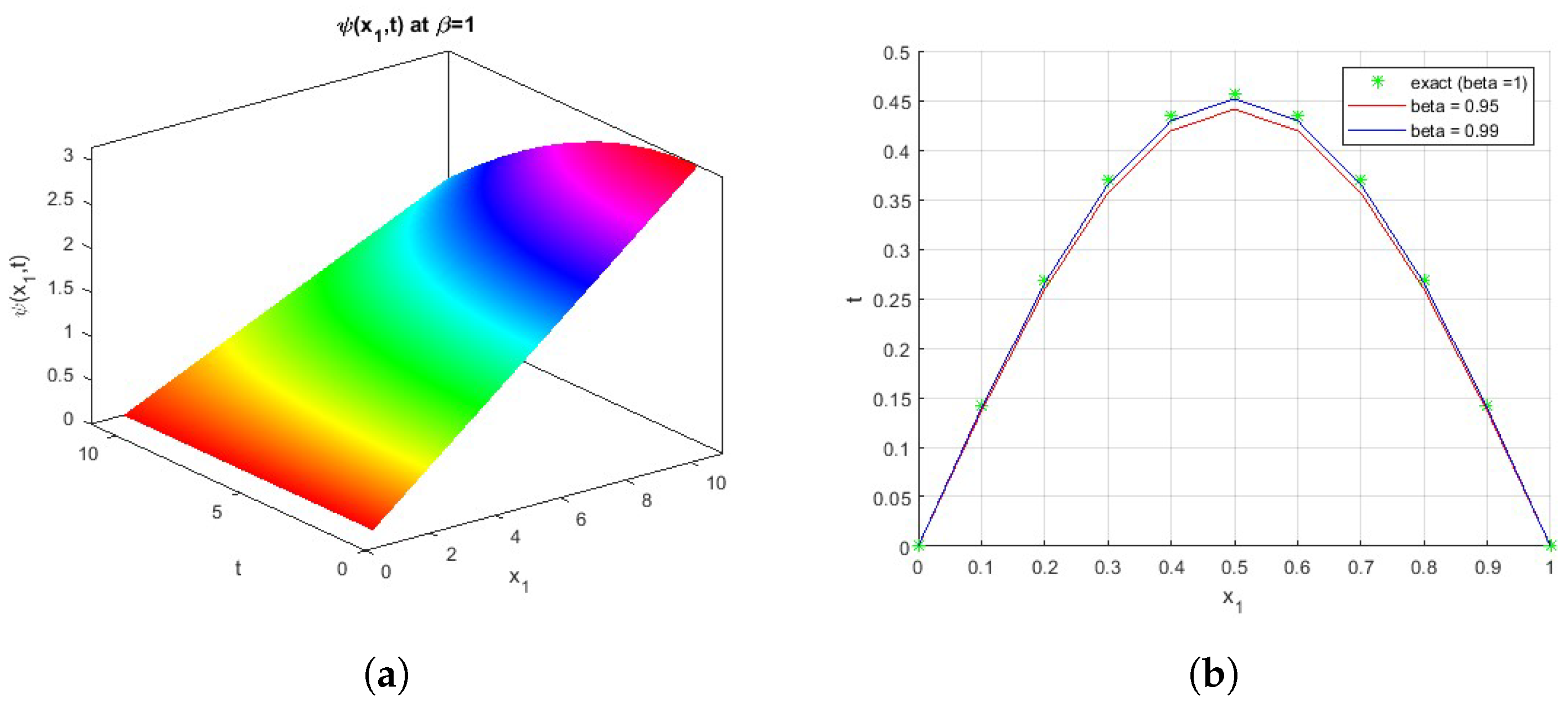
3. n + 1-Dimensional Fractional Dispersive KDV Equation and MGLTDM

In this article unit, we explain four problems of linear and nonlinear fractional dispersive PDEs of order three employing the generalized Laplace transform decomposition method.

The first problem:

Let us consider the following linear $n+1$-dimensional Kdv equation with the initial condition of

$${\displaystyle \frac{{\partial }^{\beta }\psi }{\partial t^{\beta }}}+a{\displaystyle \sum _{j=1}^n}{\displaystyle \frac{\partial \psi }{\partial x_j}}+{\displaystyle \sum _{j=1}^n}{\displaystyle \frac{{\partial }^3\psi }{\partial x_j^3}}=f(x_1,x_2,\dots ,x_n,t),t>0,0<\beta \le 1,$$

(6)

and

$$\psi (x_1,x_2,\dots ,x_n,0)=f_1(x_1,x_2,\dots ,x_n).$$

(7)

where $\psi \left(x_1,x_2,\dots ,x_n\right)$ are field variables, $x_1,x_2,\dots ,x_n\in \mathbb{R}$ are space coordinates in the propagation direction of the field and t is a time. To study the solution of Equation (6) using the MGLTDM, the following steps are discussed:

Step 1: With the assistance of MGLT, Equation (6) becomes

$$\begin{array}{ccc}& & {\displaystyle \prod _{j=1}^n}{G}_{x_j}{G}_t\left[{\displaystyle \frac{{\partial }^{\beta }\psi }{\partial t^{\beta }}}\right]+{\displaystyle \prod _{j=1}^n}{G}_{x_j}{G}_t\left[a{\displaystyle \sum _{j=1}^n}{\displaystyle \frac{\partial \psi }{\partial x_j}}+{\displaystyle \sum _{j=1}^n}{\displaystyle \frac{{\partial }^3\psi }{\partial x_j^3}}\right]\hfill \\ & =& {\displaystyle \prod _{j=1}^n}{G}_{x_j}{G}_t\left[f(x_1,x_2,\dots ,x_n,t)\right].\hfill \end{array}$$

(8)

Step 2: Employing Equation (3), we get

$$\begin{array}{ccc}& & {\displaystyle \frac{\mathsf{\Psi }\left(p_1,p_2,\dots ,p_n,s\right)}{s^{\beta }}}-{\displaystyle \frac{s^{\alpha }{F}_1\left(p_1,p_2,\dots ,p_n\right)}{s^{\beta -1}}}\hfill \\ & =& -{\displaystyle \prod _{j=1}^n}{G}_{x_j}{G}_t\left[a{\displaystyle \sum _{j=1}^n}{\displaystyle \frac{\partial \psi }{\partial x_j}}+{\displaystyle \sum _{j=1}^n}{\displaystyle \frac{{\partial }^3\psi }{\partial x_j^3}}\right]\hfill \\ & & +F\left(p_1,p_2,\dots ,p_n,s\right),\hfill \end{array}$$

(9)

where $F\left(p_1,p_2,\dots ,p_n,s\right)$ and $F_1\left(p_1,p_2,\dots ,p_n\right)$ are the (MGLT) for $f\left(x_1,x_2,\dots ,x_n,t\right)$ and $f_1\left(x_1,x_2,\dots ,x_n\right)$, respectively.

Step 3: Multiplying Equation (9) by $s^{\beta }$, we get

$$\begin{array}{ccc}\hfill \mathsf{\Psi }\left(p_1,p_2,\dots ,p_n,s\right)& =& s^{\alpha +1}{F}_1\left(p_1,p_2,\dots ,p_n\right)\hfill \\ & & -s^{\beta }{\displaystyle \prod _{j=1}^n}{G}_{x_j}{G}_t\left[a{\displaystyle \sum _{j=1}^n}{\displaystyle \frac{\partial \psi }{\partial x_j}}+{\displaystyle \sum _{j=1}^n}{\displaystyle \frac{{\partial }^3\psi }{\partial x_j^3}}\right]\hfill \\ & & +s^{\beta }F\left(p_1,p_2,\dots ,p_n,s\right).\hfill \end{array}$$

(10)

Step 4: Operating inverse multi-G Laplace transform for Equation (10),

$$\begin{array}{ccc}\hfill \psi (x_1,x_2,\dots ,x_n,t)& =& {\displaystyle \prod _{j=1}^n}{G}_{p_j}^{-1}{G}_s^{-1}\left[s^{\alpha +1}{F}_1\left(p_1,p_2,\dots ,p_n\right)\right]\hfill \\ & & +{\displaystyle \prod _{j=1}^n}{G}_{p_j}^{-1}{G}_s^{-1}\left[s^{\beta }F\left(p_1,p_2,\dots ,p_n,s\right)\right]\hfill \\ & & -{\displaystyle \prod _{j=1}^n}{G}_{p_j}^{-1}{G}_s^{-1}\left[s^{\beta }{\displaystyle \prod _{j=1}^n}{G}_{x_j}{G}_t\left[a{\displaystyle \sum _{j=1}^n}{\displaystyle \frac{\partial \psi }{\partial x_j}}+{\displaystyle \sum _{j=1}^n}{\displaystyle \frac{{\partial }^3\psi }{\partial x_j^3}}\right]\right],\hfill \end{array}$$

(11)

Step 5: Using the ADM procedure for Equation (11), we get

$$\begin{array}{ccc}\hfill {\displaystyle \sum _{m=0}^{\infty }}{\psi }_m& =& {\displaystyle \prod _{j=1}^n}{G}_{p_j}^{-1}{G}_s^{-1}\left[s^{\alpha +1}{F}_1\left(p_1,p_2,\dots ,p_n\right)+s^{\beta }F\left(p_1,p_2,\dots ,p_n,s\right)\right]\hfill \\ & & -{\displaystyle \prod _{j=1}^n}{G}_{p_j}^{-1}{G}_s^{-1}\left[s^{\beta }{\displaystyle \prod _{j=1}^n}{G}_{x_j}{G}_t\left[a{\displaystyle \sum _{j=1}^n}\left({\displaystyle \sum _{m=0}^{\infty }}{\displaystyle \frac{\partial {\psi }_m}{\partial x_j}}\right)+{\displaystyle \sum _{j=1}^n}\left({\displaystyle \sum _{m=0}^{\infty }}{\displaystyle \frac{{\partial }^3{\psi }_m}{\partial x_j^3}}\right)\right]\right],\hfill \end{array}$$

(12)

where

$${\psi }_0={\displaystyle \prod _{j=1}^n}{G}_{p_j}^{-1}{G}_s^{-1}\left[s^{\alpha +1}{F}_1\left(p_1,p_2,\dots ,p_n\right)+s^{\beta }F\left(p_1,p_2,\dots ,p_n,s\right)\right],$$

(13)

and the remaining contents are denoted by

$${\psi }_{m+1}=-{\displaystyle \prod _{j=1}^n}{G}_{p_j}^{-1}{G}_s^{-1}\left[s^{\beta }{\displaystyle \prod _{j=1}^n}{G}_{x_j}{G}_t\left[a\left({\displaystyle \sum _{j=1}^n}{\displaystyle \frac{\partial {\psi }_m}{\partial x_j}}\right)+\left({\displaystyle \sum _{j=1}^n}{\displaystyle \frac{{\partial }^3{\psi }_m}{\partial x_j^3}}\right)\right]\right].$$

(14)

The series solution of Equation (6) is given by

$$\psi ={\psi }_0+{\psi }_1+{\psi }_2+\dots$$

Suppose that the inverse exists for each term of Equations (13) and (14).

The second problem:

Let us consider the following linear one-dimensional Kdv equation with the initial condition of

$${\displaystyle \frac{{\partial }^{\beta }\psi }{\partial t^{\beta }}}+a{\displaystyle \frac{\partial \psi }{\partial x_1}}+{\displaystyle \frac{{\partial }^3\psi }{\partial x_1^3}}=f(x_1,t),t>0,0<\beta \le 1,$$

(15)

and

$$\psi (x_1,0)=f_1\left(x_1\right).$$

(16)

where $\psi \left(x_1\right)$ is a field variable, $x_1\in \mathbb{R}$ is a space coordinate in the propagation direction of the field and t is a time. In order to solve Equation (15) by utilizing the double-generalized Laplace transform decomposition method (DGLTDM), the next steps are needed:

Step 1: With the help of DGLT, Equation (15) becomes

$$G_2\left[{\displaystyle \frac{{\partial }^{\beta }\psi }{\partial t^{\beta }}}\right]+G_2\left[a{\displaystyle \frac{\partial \psi }{\partial x_1}}+{\displaystyle \frac{{\partial }^3\psi }{\partial x_1^3}}\right]=G_2\left[f(x_1,t)\right].$$

(17)

Step 2: Utilizing Equation (4), we will get

$${\displaystyle \frac{1}{s^{\beta }}}\mathsf{\Psi }\left(p_1,s\right)-{\displaystyle \frac{s^{\alpha }}{s^{\beta -1}}}{F}_1\left(p_1\right)=-G_2\left[a{\displaystyle \frac{\partial \psi }{\partial x_1}}+{\displaystyle \frac{{\partial }^3\psi }{\partial x_1^3}}\right]+F\left(p_1,s\right),$$

(18)

where $F_1\left(p_1\right)$ and $F\left(p_1,s\right)$ are the (GLT) and (DGLT) for $f\left(x_1,0\right)$ and $f\left(x_1,t\right)$, respectively.

Step 3: Multiplying Equation (18) by $s^{\beta }$, we can get

$$\mathsf{\Psi }\left(p_1,s\right)=s^{\alpha +1}{F}_1\left(p_1\right)-s^{\beta }{G}_2\left[a{\displaystyle \frac{\partial \psi }{\partial x_1}}+{\displaystyle \frac{{\partial }^3\psi }{\partial x_1^3}}\right]+s^{\beta }F\left(p_1,s\right).$$

(19)

Step 4: Operating the IDGLT for Equation (19),

$$\begin{array}{ccc}\hfill \psi \left(x_1,t\right)& =& G_2^{-1}\left[s^{\alpha +1}{F}_1\left(p_1\right)+s^{\beta }F\left(p_1,s\right)\right]\hfill \\ & & -G_2^{-1}\left[s^{\beta }{G}_2\left[a{\displaystyle \frac{\partial \psi }{\partial x_1}}+{\displaystyle \frac{{\partial }^3\psi }{\partial x_1^3}}\right]\right].\hfill \end{array}$$

(20)

Step 5: Employing the ADM procedure for Equation (11), we obtain

$$\begin{array}{ccc}\hfill {\displaystyle \sum _{m=0}^{\infty }}{\psi }_m& =& G_2^{-1}\left[s^{\alpha +1}{F}_1\left(p_1\right)+s^{\beta }F\left(p_1,s\right)\right]\hfill \\ & & -G_2^{-1}\left[s^{\beta }{G}_2\left[a{\displaystyle \sum _{m=0}^{\infty }}{\displaystyle \frac{\partial {\psi }_m}{\partial x_1}}+{\displaystyle \sum _{m=0}^{\infty }}{\displaystyle \frac{{\partial }^3{\psi }_m}{\partial x_1^3}}\right]\right],\hfill \end{array}$$

(21)

here, $m=0,1,2,3,\dots ,$ where

$${\psi }_0=G_2^{-1}\left[s^{\alpha +1}{F}_1\left(p_1\right)+s^{\beta }F\left(p_1,s\right)\right],$$

(22)

the remainder of the components are given by

$${\psi }_{m+1}=-G_2^{-1}\left[s^{\beta }{G}_2\left[a{\displaystyle \frac{\partial {\psi }_m}{\partial x_1}}+{\displaystyle \frac{{\partial }^3{\psi }_m}{\partial x_1^3}}\right]\right],$$

(23)

The series solution of Equation (15) is given by

$$\psi ={\psi }_0+{\psi }_1+{\psi }_2+\dots$$

In the following example, we apply the DGLTDM to get the solution of the fractional dispersive KdV equation:

Example 2 

([6]). The fractional dispersive KdV equation subject to the initial condition is considered as follows:

$$\begin{array}{ccc}\hfill {\displaystyle \frac{{\partial }^{\beta }\psi }{\partial t^{\beta }}}+{\displaystyle \frac{{\partial }^3\psi }{\partial x_1^3}}& =& -sin\left(\pi x_1\right)sin\left(t\right)-{\pi }^{3}cos\left(\pi x_1\right)cos\left(t\right),\hfill \\ \hfill x_1,t& >& 0,0<\beta \le 1\hfill \end{array}$$

(24)

and

$$\psi (x_1,0)=sin\left(\pi x_1\right).$$

(25)

Solution 1. 

By utilizing the DGLT of Equation (24) and using Equation (19), we get

$$\begin{array}{ccc}\hfill \mathsf{\Psi }\left(p_1,s\right)& =& {\displaystyle \frac{\pi p_1^{\alpha +2}{s}^{\alpha +1}}{1+p_1^2{\pi }^2}}-s^{\beta }{G}_2\left[{\displaystyle \frac{{\partial }^3\psi }{\partial x_1^3}}\right]\hfill \\ & & +s^{\sigma }{G}_2\left[sin\left(\pi x_1\right)sin\left(t\right)-{\pi }^{3}cos\left(\pi x_1\right)cos\left(t\right)\right],\hfill \end{array}$$

(26)

applying the  $sin\left(t\right)$ and  $cos\left(t\right)$ series in the Equation (26), we have

$$\begin{array}{ccc}\hfill \mathsf{\Psi }\left(p_1,s\right)& =& {\displaystyle \frac{\pi p_1^{\alpha +2}{s}^{\alpha +1}}{1+p_1^2{\pi }^2}}-s^{\beta }{G}_2\left[{\displaystyle \frac{{\partial }^3\psi }{\partial x_1^3}}\right]\hfill \\ & & -s^{\beta }{G}_2\left[sin\left(\pi x_1\right)\left(t-{\displaystyle \frac{t^3}{3!}}+{\displaystyle \frac{t^5}{5!}}-\dots \right)\right]\hfill \\ & & -s^{\beta }{G}_2\left[{\pi }^{3}cos\left(\pi x_1\right)\left(1-{\displaystyle \frac{t^2}{2!}}+{\displaystyle \frac{t^4}{4!}}-\dots \right)\right],\hfill \end{array}$$

(27)

$$\begin{array}{ccc}\hfill \mathsf{\Psi }\left(p_1,s\right)& =& {\displaystyle \frac{\pi p_1^{\alpha +2}{s}^{\alpha +1}}{1+p_1^2{\pi }^2}}-s^{\beta }{G}_2\left[{\displaystyle \frac{{\partial }^3\psi }{\partial x_1^3}}\right]\hfill \\ & & -{\displaystyle \frac{\pi p_1^{\alpha +2}}{1+p_1^2{\pi }^2}}\left(s^{\beta +\alpha +2}-s^{\beta +\alpha +4}+s^{\beta +\alpha +6}-\dots \right)\hfill \\ & & -\left[{\displaystyle \frac{{\pi }^3{p}_1^{\alpha +1}}{1+p_1^2{\pi }^2}}\left(s^{\beta +\alpha +1}-s^{\beta +\alpha +3}+s^{\beta +\alpha +5}-\dots \right)\right],\hfill \end{array}$$

(28)

by employing an 0IDGLT for the Equation (28) and using the ADM proceeding it, we get

$$\begin{array}{ccc}\hfill {\displaystyle \sum _{m=0}^{\infty }}{\psi }_m\left(x_1,t\right)& =& sin\left(\pi x_1\right)-sin\left(\pi x_1\right)\left({\displaystyle \frac{t^{\beta +1}}{\mathsf{\Gamma }\left(\beta +2\right)}}-{\displaystyle \frac{t^{\beta +3}}{\mathsf{\Gamma }\left(\beta +4\right)}}+{\displaystyle \frac{t^{\beta +5}}{\mathsf{\Gamma }\left(\beta +6\right)}}-\dots \right)\hfill \\ & & -{\pi }^{3}cos\left(\pi x_1\right)\left({\displaystyle \frac{t^{\beta }}{\mathsf{\Gamma }\left(\beta +1\right)}}-{\displaystyle \frac{t^{\beta +2}}{\mathsf{\Gamma }\left(\beta +3\right)}}+{\displaystyle \frac{t^{\beta +4}}{\mathsf{\Gamma }\left(\beta +5\right)}}-\dots \right)\hfill \\ & & -G_2^{-1}\left[s^{\beta }{G}_2\left[{\displaystyle \frac{{\partial }^3\psi }{\partial x_1^3}}\right]\right],\hfill \end{array}$$

$$\begin{array}{ccc}\hfill {\psi }_0\left(x_1,t\right)& =& sin\left(\pi x_1\right)-sin\left(\pi x_1\right)\left({\displaystyle \frac{t^{\beta +1}}{\mathsf{\Gamma }\left(\beta +2\right)}}-{\displaystyle \frac{t^{\beta +3}}{\mathsf{\Gamma }\left(\beta +4\right)}}+{\displaystyle \frac{t^{\beta +5}}{\mathsf{\Gamma }\left(\beta +6\right)}}-\dots \right)\hfill \\ & & -{\pi }^{3}cos\left(\pi x_1\right)\left({\displaystyle \frac{t^{\beta }}{\mathsf{\Gamma }\left(\beta +1\right)}}-{\displaystyle \frac{t^{\beta +2}}{\mathsf{\Gamma }\left(\beta +3\right)}}+{\displaystyle \frac{t^{\beta +4}}{\mathsf{\Gamma }\left(\beta +5\right)}}-\dots \right),\hfill \end{array}$$

and

$${\psi }_{m+1}\left(x_1,t\right)=-G_2^{-1}\left[s^{\beta }{G}_2\left[{\displaystyle \frac{{\partial }^3{\psi }_m}{\partial x_1^3}}\right]\right].$$

(29)

where  $m\ge 0,$ the following first two terms are denoted by

$$\begin{array}{ccc}\hfill {\psi }_1\left(x_1,t\right)& =& -G_2^{-1}\left[s^{\beta }{G}_2\left[{\displaystyle \frac{{\partial }^3{\psi }_0}{\partial x_1^3}}\right]\right]\hfill \\ & =& G_2^{-1}\left[s^{\beta }{G}_2\left[{\pi }^{3}cos\left(\pi x_1\right)\right]\right]\hfill \\ & & -G_2^{-1}\left[s^{\beta }{G}_2\left[{\pi }^{3}cos\left(\pi x_1\right)\left({\displaystyle \frac{t^{\beta +1}}{\mathsf{\Gamma }\left(\beta +2\right)}}-{\displaystyle \frac{t^{\beta +3}}{\mathsf{\Gamma }\left(\beta +4\right)}}+{\displaystyle \frac{t^{\beta +5}}{\mathsf{\Gamma }\left(\beta +6\right)}}-\dots \right)\right]\right]\hfill \\ & & +G_2^{-1}\left[s^{\beta }{G}_2\left[{\pi }^{6}sin\left(\pi x_1\right)\left({\displaystyle \frac{t^{\beta }}{\mathsf{\Gamma }\left(\beta +1\right)}}-{\displaystyle \frac{t^{\beta +2}}{\mathsf{\Gamma }\left(\beta +3\right)}}+{\displaystyle \frac{t^{\beta +4}}{\mathsf{\Gamma }\left(\beta +5\right)}}-\dots \right)\right]\right]\hfill \end{array}$$

thus,

$$\begin{array}{ccc}\hfill {\psi }_1\left(x_1,t\right)& =& G_2^{-1}\left[{\displaystyle \frac{{\pi }^3{s}^{\alpha +\beta +1}{p}_1^{\alpha +1}}{1+p_1^2{\pi }^2}}\right]\hfill \\ & & -G_2^{-1}\left[\left[{\displaystyle \frac{{\pi }^3{p}_1^{\alpha +1}}{1+p_1^2{\pi }^2}}\left(s^{\alpha +2\beta +2}-s^{\alpha +2\beta +4}+s^{\alpha +2\beta +6}-s^{\alpha +2\beta +8}+\dots \right)\right]\right]\hfill \\ & & +G_2^{-1}\left[\left[{\displaystyle \frac{{\pi }^4{p}_1^{\alpha +2}}{1+p_1^2{\pi }^2}}\left(s^{\alpha +2\beta +1}-s^{\alpha +2\beta +3}+s^{\alpha +2\beta +5}-s^{\alpha +2\beta +7}+\dots \right)\right]\right],\hfill \end{array}$$

hence,

$$\begin{array}{ccc}\hfill {\psi }_1\left(x_1,t\right)& =& {\displaystyle \frac{{\pi }^3{t}^{\beta }}{\mathsf{\Gamma }\left(\beta +1\right)}}cos\left(\pi x_1\right)\hfill \\ & & -{\pi }^{3}cos\left(\pi x_1\right)\left[\left({\displaystyle \frac{t^{2\beta +1}}{\mathsf{\Gamma }\left(2\beta +2\right)}}-{\displaystyle \frac{t^{2\beta +3}}{\mathsf{\Gamma }\left(2\beta +4\right)}}+{\displaystyle \frac{t^{2\beta +5}}{\mathsf{\Gamma }\left(2\beta +6\right)}}-\dots \right)\right]\hfill \\ & & +{\pi }^{6}sin\left(\pi x_1\right)\left({\displaystyle \frac{t^{2\beta }}{\mathsf{\Gamma }\left(2\beta +1\right)}}-{\displaystyle \frac{t^{2\beta +2}}{\mathsf{\Gamma }\left(2\beta +3\right)}}+{\displaystyle \frac{t^{2\beta +4}}{\mathsf{\Gamma }\left(2\beta +5\right)}}-\dots \right),\hfill \end{array}$$

at  $m=1,$ we have

$$\begin{array}{ccc}\hfill {\psi }_2\left(x_1,t\right)& =& -G_2^{-1}\left[s^{\beta }{G}_2\left[{\displaystyle \frac{{\partial }^3{\psi }_1}{\partial x_1^3}}\right]\right]\hfill \\ & =& -G_2^{-1}\left[s^{\beta }{G}_2\left[{\pi }^6{\displaystyle \frac{t^{\beta }}{\mathsf{\Gamma }\left(\beta +1\right)}}sin\left(\pi x_1\right)\right]\right]\hfill \\ & & -G_2^{-1}\left[s^{\beta }{G}_2\left[{\pi }^{6}sin\left(\pi x_1\right)\left({\displaystyle \frac{t^{2\beta +1}}{\mathsf{\Gamma }\left(2\beta +2\right)}}-{\displaystyle \frac{t^{2\beta +3}}{\mathsf{\Gamma }\left(2\beta +4\right)}}+{\displaystyle \frac{t^{2\beta +5}}{\mathsf{\Gamma }\left(2\beta +6\right)}}-\dots \right)\right]\right]\hfill \\ & & -G_2^{-1}\left[s^{\beta }{G}_2\left[{\pi }^{9}cos\left(\pi x_1\right)\left({\displaystyle \frac{t^{2\beta }}{\mathsf{\Gamma }\left(2\beta +1\right)}}-{\displaystyle \frac{t^{2\beta +2}}{\mathsf{\Gamma }\left(2\beta +3\right)}}+{\displaystyle \frac{t^{2\beta +4}}{\mathsf{\Gamma }\left(2\beta +5\right)}}-\dots \right)\right]\right],\hfill \\ \hfill {\psi }_2\left(x_1,t\right)& =& -{\displaystyle \frac{{\pi }^6{t}^{2\beta }}{\mathsf{\Gamma }\left(2\beta +1\right)}}\left(sin\left(\pi x_1\right)+{\pi }^{6}sin\left(\pi x_1\right)\right)\hfill \\ & & \times \left[\left({\displaystyle \frac{t^{3\beta +1}}{\mathsf{\Gamma }\left(3\beta +2\right)}}-{\displaystyle \frac{t^{3\beta +3}}{\mathsf{\Gamma }\left(3\beta +4\right)}}+{\displaystyle \frac{t^{3\beta +5}}{\mathsf{\Gamma }\left(3\beta +6\right)}}-\dots \right)\right]\hfill \\ & & +{\pi }^{9}cos\left(\pi x_1\right)\left({\displaystyle \frac{t^{3\beta }}{\mathsf{\Gamma }\left(3\beta +1\right)}}-{\displaystyle \frac{t^{3\beta +2}}{\mathsf{\Gamma }\left(3\beta +3\right)}}+{\displaystyle \frac{t^{3\beta +4}}{\mathsf{\Gamma }\left(3\beta +5\right)}}-\dots \right).\hfill \end{array}$$

We examine, the approximate solution of Equation (24) as the following:

$$\begin{array}{ccc}\hfill \psi \left(x_1,t\right)& =& sin\left(\pi x_1\right)-sin\left(\pi x_1\right)\left({\displaystyle \frac{t^{\beta +1}}{\mathsf{\Gamma }\left(\beta +2\right)}}-{\displaystyle \frac{t^{\beta +3}}{\mathsf{\Gamma }\left(\beta +4\right)}}+{\displaystyle \frac{t^{\beta +5}}{\mathsf{\Gamma }\left(\beta +6\right)}}-\dots \right)\hfill \\ & & -{\pi }^{3}cos\left(\pi x_1\right)\left({\displaystyle \frac{t^{\beta }}{\mathsf{\Gamma }\left(\beta +1\right)}}-{\displaystyle \frac{t^{\beta +2}}{\mathsf{\Gamma }\left(\beta +3\right)}}+{\displaystyle \frac{t^{\beta +4}}{\mathsf{\Gamma }\left(\beta +5\right)}}-\dots \right)\hfill \\ & & +{\displaystyle \frac{{\pi }^3{t}^{\beta }}{\mathsf{\Gamma }\left(\beta +1\right)}}cos\left(\pi x_1\right)\hfill \\ & & -{\pi }^{3}cos\left(\pi x_1\right)\times \left({\displaystyle \frac{t^{2\beta +1}}{\mathsf{\Gamma }\left(2\beta +2\right)}}-{\displaystyle \frac{t^{2\beta +3}}{\mathsf{\Gamma }\left(2\beta +4\right)}}+{\displaystyle \frac{t^{2\beta +5}}{\mathsf{\Gamma }\left(2\beta +6\right)}}-\dots \right)\hfill \\ & & +{\pi }^{6}sin\left(\pi x_1\right)\left({\displaystyle \frac{t^{2\beta }}{\mathsf{\Gamma }\left(2\beta +1\right)}}-{\displaystyle \frac{t^{2\beta +2}}{\mathsf{\Gamma }\left(2\beta +3\right)}}+{\displaystyle \frac{t^{2\beta +4}}{\mathsf{\Gamma }\left(2\beta +5\right)}}-\dots \right)\hfill \\ & & -{\displaystyle \frac{{\pi }^6{t}^{2\beta }}{\mathsf{\Gamma }\left(2\beta +1\right)}}sin\left(\pi x_1\right)+{\pi }^{6}sin\left(\pi x_1\right)\hfill \\ & & \times \left[\left({\displaystyle \frac{t^{3\beta +1}}{\mathsf{\Gamma }\left(3\beta +2\right)}}-{\displaystyle \frac{t^{3\beta +3}}{\mathsf{\Gamma }\left(3\beta +4\right)}}+{\displaystyle \frac{t^{3\beta +5}}{\mathsf{\Gamma }\left(3\beta +6\right)}}-\dots \right)\right]\hfill \\ & & +{\pi }^{9}cos\left(\pi x_1\right)\left({\displaystyle \frac{t^{3\beta }}{\mathsf{\Gamma }\left(3\beta +1\right)}}-{\displaystyle \frac{t^{3\beta +2}}{\mathsf{\Gamma }\left(3\beta +3\right)}}+{\displaystyle \frac{t^{3\beta +4}}{\mathsf{\Gamma }\left(3\beta +5\right)}}-\dots \right)\hfill \end{array}$$

Thus, the precise solution at  $\beta =1$ is described by

$$\begin{array}{ccc}\hfill \psi \left(x,t\right)& =& sin\left(\pi x_1\right)-sin\left(\pi x_1\right)\left({\displaystyle \frac{t^2}{\mathsf{\Gamma }\left(3\right)}}-{\displaystyle \frac{t^4}{\mathsf{\Gamma }\left(5\right)}}+{\displaystyle \frac{t^6}{\mathsf{\Gamma }\left(7\right)}}-\dots \right)\hfill \\ & & -{\pi }^{3}cos\left(\pi x_1\right)\left({\displaystyle \frac{t}{\mathsf{\Gamma }\left(2\right)}}-{\displaystyle \frac{t^3}{\mathsf{\Gamma }\left(4\right)}}+{\displaystyle \frac{t^{\sigma 5}}{\mathsf{\Gamma }\left(6\right)}}-\dots \right)\hfill \\ & & +{\displaystyle \frac{{\pi }^{3}t}{\mathsf{\Gamma }\left(2\right)}}cos\left(\pi x_1\right)-{\pi }^{3}cos\left(\pi x_1\right)\left[\left({\displaystyle \frac{t^3}{\mathsf{\Gamma }\left(4\right)}}-{\displaystyle \frac{t^5}{\mathsf{\Gamma }\left(6\right)}}+{\displaystyle \frac{t^7}{\mathsf{\Gamma }\left(8\right)}}-\dots \right)\right]\hfill \\ & & +{\pi }^{6}sin\left(\pi x_1\right)\left({\displaystyle \frac{t^2}{\mathsf{\Gamma }\left(3\right)}}-{\displaystyle \frac{t^4}{\mathsf{\Gamma }\left(5\right)}}+{\displaystyle \frac{t^6}{\mathsf{\Gamma }\left(7\right)}}-{\displaystyle \frac{t^8}{\mathsf{\Gamma }\left(9\right)}}+\dots \right)\hfill \\ & & -{\displaystyle \frac{{\pi }^6{t}^2}{\mathsf{\Gamma }\left(3\right)}}sin\left(\pi x_1\right)+{\pi }^{6}sin\left(\pi x_1\right)\left[\left({\displaystyle \frac{t^4}{\mathsf{\Gamma }\left(5\right)}}-{\displaystyle \frac{t^6}{\mathsf{\Gamma }\left(7\right)}}+{\displaystyle \frac{t^8}{\mathsf{\Gamma }\left(9\right)}}-\dots \right)\right]\hfill \\ & & +{\pi }^{9}cos\left(\pi x_1\right)\left({\displaystyle \frac{t^3}{\mathsf{\Gamma }\left(4\right)}}-{\displaystyle \frac{t^5}{\mathsf{\Gamma }\left(6\right)}}+{\displaystyle \frac{t^7}{\mathsf{\Gamma }\left(8\right)}}-\dots \right).\hfill \end{array}$$

By simplifying,

$$\begin{array}{ccc}\hfill \psi \left(x_1,t\right)& =& sin\left(\pi x_1\right)-sin\left(\pi x_1\right)\left({\displaystyle \frac{t^2}{\mathsf{\Gamma }\left(3\right)}}-{\displaystyle \frac{t^4}{\mathsf{\Gamma }\left(5\right)}}+{\displaystyle \frac{t^6}{\mathsf{\Gamma }\left(7\right)}}-{\displaystyle \frac{t^8}{\mathsf{\Gamma }\left(7\right)}}+\dots \right)\hfill \\ & =& sin\left(\pi x_1\right)\left(1-{\displaystyle \frac{t^2}{\mathsf{\Gamma }\left(3\right)}}+{\displaystyle \frac{t^4}{\mathsf{\Gamma }\left(5\right)}}-{\displaystyle \frac{t^6}{\mathsf{\Gamma }\left(7\right)}}+{\displaystyle \frac{t^8}{\mathsf{\Gamma }\left(7\right)}}-\dots \right),\hfill \end{array}$$

$$\psi \left(x_1,t\right)=sin\left(\pi x_1\right)cos\left(t\right).$$

Figure 1a introduces a comparison between the exact solution and the obtained numerical solution of Equation (24). At t = 1 and $\beta =1$ the exact solution is gained. By taking diverse values of $\beta$, such as ($\beta =0.95$, $\beta =0.99$), we get the approximate solutions. Figure 1b shows the plot of function $\psi (x_1,t)$ in two dimensions.

Figure 1. (a): Comparison between exact and numerical solutions. (b): The surface of the function $\psi (x_1,t)$.

Table 1 shows the numerical solution for different values of β for the function $\psi (x_1,t)$.

Table 1. Compression between exact and approximation solutions.

Exact	The Method	Error	The Method	Error
β = 1	β = 0.95		β = 0.99
0	0	0	0	0
0.1412	0.1363	0.0049	0.1396	0.0016
0.2686	0.2592	0.0094	0.2655	0.0031
0.3697	0.3568	0.0129	0.3654	0.0043
0.4346	0.4194	0.0152	0.4296	0.0050
0.4570	0.4410	0.0159	0.4517	0.0053
0.4346	0.4194	0.0152	0.4296	0.0050
0.3697	0.3568	0.0129	0.3654	0.0043
0.2686	0.2592	0.0094	0.2655	0.0031
0.1412	0.1363	0.0049	0.1396	0.0016
0.0000	0.0000	0.0000	0.0000	0.0000

Table 1. Compression between exact and approximation solutions.

Exact	The Method	Error	The Method	Error
β = 1	β = 0.95		β = 0.99
0	0	0	0	0
0.1412	0.1363	0.0049	0.1396	0.0016
0.2686	0.2592	0.0094	0.2655	0.0031
0.3697	0.3568	0.0129	0.3654	0.0043
0.4346	0.4194	0.0152	0.4296	0.0050
0.4570	0.4410	0.0159	0.4517	0.0053
0.4346	0.4194	0.0152	0.4296	0.0050
0.3697	0.3568	0.0129	0.3654	0.0043
0.2686	0.2592	0.0094	0.2655	0.0031
0.1412	0.1363	0.0049	0.1396	0.0016
0.0000	0.0000	0.0000	0.0000	0.0000

In the following, we plan some significant evidence about the triple-G Laplace transform decomposition method (TGLTDM) to solve the linear fractional dispersive PDE of order three.

The third problem:

Consider the following linear two-dimensional Kdv equation with the initial condition of

$${\displaystyle \frac{{\partial }^{\beta }\psi }{\partial t^{\beta }}}+a{\displaystyle \frac{{\partial }^3\psi }{\partial x_1^3}}+b{\displaystyle \frac{{\partial }^3\psi }{\partial x_2^3}}=f(x_1,x_2,t),x_1,x_2,t>0,0<\sigma \le 1,$$

(30)

and

$$\psi (x_1,x_2,0)=f_1(x_1,x_2),$$

(31)

where a and b are constant. To gain the solution of Equation (30), the triple-generalized Laplace transform decomposition method (TGLTDM) and the next steps are suggested:

Step 1: Upon utilizing TGLT for Equation (30) and DGLT for Equation (31), we get

$$G_3\left[{\displaystyle \frac{{\partial }^{\beta }\psi }{\partial t^{\beta }}}\right]+G_3\left[a{\displaystyle \frac{{\partial }^3\psi }{\partial x_1^3}}+b{\displaystyle \frac{{\partial }^3\psi }{\partial x_2^3}}\right]=G_3\left[f(x_1,x_2,t)\right],$$

(32)

where the symbols $G_3=G_{x_1}{G}_{x_2}{G}_t$ denote TGLT.

Step 2: Implementing Equation (4), we obtain

$${\displaystyle \frac{1}{s^{\beta }}}\mathsf{\Psi }\left(p_1,p_2,s\right)-{\displaystyle \frac{s^{\alpha }}{s^{\beta -1}}}{F}_1\left(p_1,p_2\right)=-G_3\left[a{\displaystyle \frac{{\partial }^3\psi }{\partial x_1^3}}+b{\displaystyle \frac{{\partial }^3\psi }{\partial x_2^3}}\right]+F\left(p_1,p_2,s\right),$$

(33)

where $F_1\left(p_1,p_2\right)$ and $F\left(p_1,p_2,s\right)$ are the DGLT and TGLT for $f\left(x_1,x_2,0\right)$ and $f\left(x_1,x_2,t\right)$, respectively.

Step 3: By multiplying Equation (33) by $s^{\beta }$, we have

$$\mathsf{\Psi }\left(p_1,p_2,s\right)=s^{\alpha +1}{F}_1\left(p_1,p_2\right)-s^{\beta }{G}_3\left[a{\displaystyle \frac{{\partial }^3\psi }{\partial x_1^3}}+b{\displaystyle \frac{{\partial }^3\psi }{\partial x_2^3}}\right]+s^{\beta }F\left(p_1,p_2,s\right).$$

(34)

Step 4: Applying ITGLT for Equation (34), we obtain

$$\psi \left(x_1,x_2,t\right)=G_3^{-1}\left[s^{\alpha +1}{F}_1\left(p_1,p_2\right)+s^{\beta }F\left(p_1,p_2,s\right)\right]-G_3^{-1}\left[s^{\beta }{G}_3\left[a{\displaystyle \frac{{\partial }^3\psi }{\partial x_1^3}}+b{\displaystyle \frac{{\partial }^3\psi }{\partial x_2^3}}\right]\right],$$

(35)

where the symbol $G_3^{-1}$ indicates ITGLT.

Step 5: By employing the ADM for Equation (35),

$$\begin{array}{ccc}\hfill {\displaystyle \sum _{m=0}^{\infty }}{\psi }_m& =& G_3^{-1}\left[s^{\alpha +1}{F}_1\left(p_1,p_2\right)+s^{\beta }F\left(p_1,p_2,s\right)\right]\hfill \\ & & -G_3^{-1}\left[s^{\beta }{G}_3\left[a{\displaystyle \sum _{m=0}^{\infty }}{\displaystyle \frac{{\partial }^3{\psi }_m}{\partial x_1^3}}+b{\displaystyle \sum _{n=0}^{\infty }}{\displaystyle \frac{{\partial }^3{\psi }_m}{\partial x_2^3}}\right]\right].\hfill \end{array}$$

(36)

Then, we determine the recurrence connections as

$${\psi }_0=G_3^{-1}\left[s^{\alpha +1}{F}_1\left(p_1,p_2\right)+s^{\beta }F\left(p_1,p_2,s\right)\right],$$

(37)

and

$${\psi }_{m+1}=-G_3^{-1}\left[s^{\beta }{G}_3\left[a{\displaystyle \sum _{m=0}^{\infty }}{\displaystyle \frac{{\partial }^3{\psi }_m}{\partial x_1^3}}+b{\displaystyle \sum _{n=0}^{\infty }}{\displaystyle \frac{{\partial }^3{\psi }_m}{\partial x_2^3}}\right]\right],$$

(38)

and the series solution is given by

$$\psi ={\psi }_0+{\psi }_1+{\psi }_2+\dots$$

Example 3. 

The time-fractional dispersive KdV equation is two dimensional with the initial condition accorded by

$$\begin{array}{ccc}\hfill {\displaystyle \frac{{\partial }^{\beta }\psi }{\partial t^{\beta }}}+{\displaystyle \frac{{\partial }^3\psi }{\partial x_1^3}}+{\displaystyle \frac{{\partial }^3\psi }{\partial x_2^3}}& =& sin\left(x_1+x_2\right)cos\left(t\right)-2cos\left(x_1+x_2\right)sin\left(t\right),x_1,x_2,t>0,\hfill \\ \hfill 0& <& \beta \le 1\hfill \end{array}$$

(39)

and

$$\psi (x_1,x_2,0)=0.$$

(40)

Solution 2. 

With the assistance of Equations (37) and (38), we arrive at

$$\begin{array}{ccc}\hfill {\psi }_0& =& G_3^{-1}\left[\left({\displaystyle \frac{\left(p_1+p_2\right)p_1^{\alpha +1}{p}_2^{\alpha +1}}{\left(1+p_1^2\right)\left(1+p_2^2\right)}}\left(s^{\alpha +\beta +1}-s^{\alpha +\beta +3}+s^{\alpha +\beta +5}-\dots \right)\right)\right]\hfill \\ & & -G_3^{-1}\left[\left({\displaystyle \frac{2\left(1-p_1{p}_2\right)p_1^{\alpha +1}{p}_2^{\alpha +1}}{\left(1+p_1^2\right)\left(1+p_2^2\right)}}\left(s^{\alpha +\beta +2}-s^{\alpha +\beta +4}+s^{\alpha +\beta +6}-\dots \right)\right)\right],\hfill \end{array}$$

(41)

$${\psi }_{m+1}=-G_3^{-1}\left[s^{\beta }{G}_3\left[{\displaystyle \frac{{\partial }^3{\psi }_m}{\partial x_1^3}}+{\displaystyle \frac{{\partial }^3{\psi }_m}{\partial x_2^3}}\right]\right],$$

(42)

$$\begin{array}{ccc}\hfill {\psi }_0& =& sin\left(x_1+x_2\right)\left({\displaystyle \frac{t^{\beta }}{\mathsf{\Gamma }\left(\beta +1\right)}}-{\displaystyle \frac{t^{\beta +2}}{\mathsf{\Gamma }\left(\beta +3\right)}}+{\displaystyle \frac{t^{\beta +4}}{\mathsf{\Gamma }\left(\beta +5\right)}}-\dots \right)\hfill \\ & & -2cos\left(x_1+x_2\right)\left({\displaystyle \frac{t^{\beta +1}}{\mathsf{\Gamma }\left(\beta +2\right)}}-{\displaystyle \frac{t^{\beta +3}}{\mathsf{\Gamma }\left(\beta +4\right)}}+{\displaystyle \frac{t^{\beta +5}}{\mathsf{\Gamma }\left(\beta +6\right)}}-\dots \right),\hfill \end{array}$$

where  $m\ge 0.$ The rest terms are denoted by,

$$\begin{array}{ccc}\hfill {\psi }_1& =& -G_3^{-1}\left[s^{\beta }{G}_3\left[{\displaystyle \frac{{\partial }^3{\psi }_0}{\partial x_1^3}}+{\displaystyle \frac{{\partial }^3{\psi }_0}{\partial x_2^3}}\right]\right]\hfill \\ & =& G_3^{-1}\left[s^{\beta }{G}_3\left[2cos\left(x_1+x_2\right)\left[\mathsf{\Lambda }\right]+4sin\left(x_1+x_2\right)\left[\mathsf{{\rm Y}}\right]\right]\right],\hfill \end{array}$$

where

$$\begin{array}{ccc}\hfill \mathsf{\Lambda }& =& \left({\displaystyle \frac{t^{\beta }}{\mathsf{\Gamma }\left(\beta +1\right)}}-{\displaystyle \frac{t^{\beta +2}}{\mathsf{\Gamma }\left(\beta +3\right)}}+{\displaystyle \frac{t^{\beta +4}}{\mathsf{\Gamma }\left(\beta +5\right)}}-{\displaystyle \frac{t^{\beta +6}}{\mathsf{\Gamma }\left(\beta +7\right)}}+\dots \right),\hfill \\ \hfill \mathsf{{\rm Y}}& =& \left({\displaystyle \frac{t^{\beta +1}}{\mathsf{\Gamma }\left(\beta +2\right)}}-{\displaystyle \frac{t^{\beta +3}}{\mathsf{\Gamma }\left(\beta +4\right)}}+{\displaystyle \frac{t^{\beta +5}}{\mathsf{\Gamma }\left(\beta +6\right)}}-{\displaystyle \frac{t^{\beta +7}}{\mathsf{\Gamma }\left(\beta +8\right)}}+\dots \right).\hfill \end{array}$$

The first three terms are given by

$$\begin{array}{ccc}\hfill {\psi }_1& =& G_3^{-1}\left[{\displaystyle \frac{2\left(1-p_1{p}_2\right)p_1^{\alpha +1}{p}_2^{\alpha +1}}{\left(1+p_1^2\right)\left(1+p_2^2\right)}}\left[\left(s^{\alpha +2\beta +1}-s^{\alpha +2\beta +3}+s^{\alpha +2\beta +5}-s^{\alpha +2\beta +7}+\dots \right)\right]\right]\hfill \\ & & +G_3^{-1}\left[{\displaystyle \frac{2\left(p_1+p_2\right)p_1^{\alpha +1}{p}_2^{\alpha +1}}{\left(1+p_1^2\right)\left(1+p_2^2\right)}}\left(s^{\alpha +2\beta +2}-s^{\alpha +2\beta +4}+s^{\alpha +2\beta +6}-s^{\alpha +2\beta +8}+\dots \right)\right],\hfill \\ & =& 2cos\left(x_1+x_2\right)\left({\displaystyle \frac{t^{2\beta }}{\mathsf{\Gamma }\left(2\beta +1\right)}}-{\displaystyle \frac{t^{2\beta +2}}{\mathsf{\Gamma }\left(2\beta +3\right)}}+{\displaystyle \frac{t^{2\beta +4}}{\mathsf{\Gamma }\left(2\beta +5\right)}}-{\displaystyle \frac{t^{2\beta +6}}{\mathsf{\Gamma }\left(2\beta +7\right)}}+\dots \right)\hfill \\ & & +4sin\left(x_1+x_2\right)\left({\displaystyle \frac{t^{2\beta +1}}{\mathsf{\Gamma }\left(2\beta +2\right)}}-{\displaystyle \frac{t^{2\beta +3}}{\mathsf{\Gamma }\left(2\beta +4\right)}}+{\displaystyle \frac{t^{2\beta +5}}{\mathsf{\Gamma }\left(2\beta +6\right)}}-{\displaystyle \frac{t^{2\beta +7}}{\mathsf{\Gamma }\left(2\beta +8\right)}}+\dots \right),\hfill \end{array}$$

$$\begin{array}{ccc}\hfill {\psi }_2& =& -G_3^{-1}\left[s^{\beta }{G}_3\left[{\displaystyle \frac{{\partial }^3{\psi }_1}{\partial x_1^3}}+{\displaystyle \frac{{\partial }^3{\psi }_1}{\partial x_2^3}}\right]\right]\hfill \\ & =& -4sin\left(x_1+x_2\right)\left({\displaystyle \frac{t^{3\beta }}{\mathsf{\Gamma }\left(3\beta +1\right)}}-{\displaystyle \frac{t^{3\beta +2}}{\mathsf{\Gamma }\left(3\beta +3\right)}}+{\displaystyle \frac{t^{3\beta +4}}{\mathsf{\Gamma }\left(3\beta +5\right)}}-{\displaystyle \frac{t^{3\beta +6}}{\mathsf{\Gamma }\left(3\beta +7\right)}}+\dots \right)\hfill \\ & & +8cos\left(x_1+x_2\right)\left({\displaystyle \frac{t^{3\beta +1}}{\mathsf{\Gamma }\left(3\beta +2\right)}}-{\displaystyle \frac{t^{3\beta +3}}{\mathsf{\Gamma }\left(3\beta +4\right)}}+{\displaystyle \frac{t^{3\beta +5}}{\mathsf{\Gamma }\left(3\beta +6\right)}}-{\displaystyle \frac{t^{3\beta +7}}{\mathsf{\Gamma }\left(3\beta +8\right)}}+\dots \right),\hfill \end{array}$$

$$\begin{array}{ccc}\hfill {\psi }_3& =& -G_3^{-1}\left[s^{\beta }{G}_3\left[{\displaystyle \frac{{\partial }^3{\psi }_2}{\partial x_1^3}}+{\displaystyle \frac{{\partial }^3{\psi }_2}{\partial x_2^3}}\right]\right]\hfill \\ & =& -8cos\left(x_1+x_2\right)\left({\displaystyle \frac{t^{4\beta }}{\mathsf{\Gamma }\left(4\beta +1\right)}}-{\displaystyle \frac{t^{4\beta +2}}{\mathsf{\Gamma }\left(4\beta +3\right)}}+{\displaystyle \frac{t^{4\beta +4}}{\mathsf{\Gamma }\left(4\beta +5\right)}}-{\displaystyle \frac{t^{4\beta +6}}{\mathsf{\Gamma }\left(4\beta +7\right)}}+\dots \right)\hfill \\ & & -16sin\left(x_1+x_2\right)\left({\displaystyle \frac{t^{4\beta +1}}{\mathsf{\Gamma }\left(4\beta +2\right)}}-{\displaystyle \frac{t^{4\beta +3}}{\mathsf{\Gamma }\left(4\beta +4\right)}}+{\displaystyle \frac{t^{4\beta +5}}{\mathsf{\Gamma }\left(4\beta +6\right)}}-{\displaystyle \frac{t^{4\beta +7}}{\mathsf{\Gamma }\left(4\beta +8\right)}}+\dots \right),\hfill \end{array}$$

and so on. By adding the above iterations, the solution becomes

$$\begin{array}{ccc}\hfill \psi (x_1,x_2,t)& =& sin\left(x_1+x_2\right)\left({\displaystyle \frac{t^{\beta }}{\mathsf{\Gamma }\left(\beta +1\right)}}-{\displaystyle \frac{t^{\beta +2}}{\mathsf{\Gamma }\left(\beta +3\right)}}+{\displaystyle \frac{t^{\beta +4}}{\mathsf{\Gamma }\left(\beta +5\right)}}-\dots \right)\hfill \\ & & -2cos\left(x_1+x_2\right)\left({\displaystyle \frac{t^{\beta +1}}{\mathsf{\Gamma }\left(\beta +2\right)}}-{\displaystyle \frac{t^{\beta +3}}{\mathsf{\Gamma }\left(\beta +4\right)}}+{\displaystyle \frac{t^{\beta +5}}{\mathsf{\Gamma }\left(\beta +6\right)}}-\dots \right)\hfill \\ & & +2cos\left(x_1+x_2\right)\left({\displaystyle \frac{t^{2\beta }}{\mathsf{\Gamma }\left(2\beta +1\right)}}-{\displaystyle \frac{t^{2\beta +2}}{\mathsf{\Gamma }\left(2\beta +3\right)}}+{\displaystyle \frac{t^{2\beta +4}}{\mathsf{\Gamma }\left(2\beta +5\right)}}-\dots \right)\hfill \\ & & +4sin\left(x_1+x_2\right)\left({\displaystyle \frac{t^{2\beta +1}}{\mathsf{\Gamma }\left(2\beta +2\right)}}-{\displaystyle \frac{t^{2\beta +3}}{\mathsf{\Gamma }\left(2\beta +4\right)}}+{\displaystyle \frac{t^{2\beta +5}}{\mathsf{\Gamma }\left(2\beta +6\right)}}-\dots \right)\hfill \\ & & -4sin\left(x_1+x_2\right)\left({\displaystyle \frac{t^{3\beta }}{\mathsf{\Gamma }\left(3\beta +1\right)}}-{\displaystyle \frac{t^{3\beta +2}}{\mathsf{\Gamma }\left(3\beta +3\right)}}+{\displaystyle \frac{t^{3\beta +4}}{\mathsf{\Gamma }\left(3\beta +5\right)}}-\dots \right)\hfill \\ & & +8cos\left(x_1+x_2\right)\left({\displaystyle \frac{t^{3\beta +1}}{\mathsf{\Gamma }\left(3\beta +2\right)}}-{\displaystyle \frac{t^{3\beta +3}}{\mathsf{\Gamma }\left(3\beta +4\right)}}+{\displaystyle \frac{t^{3\beta +5}}{\mathsf{\Gamma }\left(3\beta +6\right)}}-\dots \right)\hfill \\ & & -8cos\left(x_1+x_2\right)\left({\displaystyle \frac{t^{4\beta }}{\mathsf{\Gamma }\left(4\beta +1\right)}}-{\displaystyle \frac{t^{4\beta +2}}{\mathsf{\Gamma }\left(4\beta +3\right)}}+{\displaystyle \frac{t^{4\beta +4}}{\mathsf{\Gamma }\left(4\beta +5\right)}}-\dots \right)\hfill \\ & & -16sin\left(x_1+x_2\right)\left({\displaystyle \frac{t^{4\beta +1}}{\mathsf{\Gamma }\left(4\beta +2\right)}}-{\displaystyle \frac{t^{4\beta +3}}{\mathsf{\Gamma }\left(4\beta +4\right)}}+{\displaystyle \frac{t^{4\beta +5}}{\mathsf{\Gamma }\left(4\beta +6\right)}}-\dots \right).\hfill \end{array}$$

In the special case when  $\beta =1$, the solution of Equation (39) becomes

$$\begin{array}{ccc}\hfill \psi (x_1,x_2,t)& =& sin\left(x_1+x_2\right)\left({\displaystyle \frac{t}{\mathsf{\Gamma }\left(2\right)}}-{\displaystyle \frac{t^3}{\mathsf{\Gamma }\left(4\right)}}+{\displaystyle \frac{t^5}{\mathsf{\Gamma }\left(6\right)}}-{\displaystyle \frac{t^7}{\mathsf{\Gamma }\left(8\right)}}+\dots \right),\hfill \\ & =& sin\left(x_1+x_2\right)sin\left(t\right).\hfill \end{array}$$

Table 2 shows the numerical solution for different values of β for the function $\psi (x_1,x_2,t).$

Table 2. Compression between exact and approximation solutions.

Exact	The Method	Error	The Method	Error
β = 1	β = 0.95		β = 0.99
0	0	0	0	0
0.1672	0.1693	0.0021	0.1676	0.0004
0.3277	0.3318	0.0041	0.3286	0.0009
0.4751	0.4811	0.0059	0.4764	0.0013
0.6036	0.6112	0.0075	0.6052	0.0016
0.7081	0.7169	0.0088	0.7100	0.0019
0.7843	0.7941	0.0098	0.7864	0.0021
0.8292	0.8396	0.0104	0.8314	0.0022
0.8411	0.8516	0.0105	0.8433	0.0022
0.8195	0.8297	0.0102	0.8216	0.0022
0.7651	0.7747	0.0096	0.7672	0.0020

Table 2. Compression between exact and approximation solutions.

Exact	The Method	Error	The Method	Error
β = 1	β = 0.95		β = 0.99
0	0	0	0	0
0.1672	0.1693	0.0021	0.1676	0.0004
0.3277	0.3318	0.0041	0.3286	0.0009
0.4751	0.4811	0.0059	0.4764	0.0013
0.6036	0.6112	0.0075	0.6052	0.0016
0.7081	0.7169	0.0088	0.7100	0.0019
0.7843	0.7941	0.0098	0.7864	0.0021
0.8292	0.8396	0.0104	0.8314	0.0022
0.8411	0.8516	0.0105	0.8433	0.0022
0.8195	0.8297	0.0102	0.8216	0.0022
0.7651	0.7747	0.0096	0.7672	0.0020

Figure 2a presents a comparison between the exact solution and the gained numerical solution of Equation (39); at t = 1 and $\beta =1$, the exact solution is obtained; by taking various values of $\beta$, such as ($\beta =0.95$, $\beta =0.99$), the approximate solution is acquired. Figure 2b shows the plot of function $\psi (x_1,x_2,t)$ with $x_2=0$ in three-dimensions.

Figure 2. (a): A comparison between exact and numerical solutions. (b): The surface of the function $\psi (x_1,t)$.

The fourth problem:

In this part, we offered the DGLTDM to solve the nonlinear one-dimensional fractional KDV equation.

Now, let us consider the nonlinear (1 + 1) dimensional fractional dispersive KDV equation having the initial condition determined by

$${\displaystyle \frac{{\partial }^{\beta }\psi }{\partial t^{\beta }}}+a{\displaystyle \frac{{\partial }^3\psi }{\partial x_1^3}}+b\psi {\displaystyle \frac{\partial \psi }{\partial x_1}}=f(x_1,t),$$

(43)

and

$$\psi \left(x_1,0\right)=f_1\left(x_1\right).$$

(44)

where $f(x_1,t)$ and $f_1\left(x_1\right)$ are defined, a and b are constants. To get the solution of Equation (43) the past examination method is suggested as follows:

$$\psi \left(x_1,t\right)=G_2^{-1}\left[s^{\alpha +1}{F}_1\left(p_1\right)+s^{\beta }F\left(p_1,s\right)\right]-G_2^{-1}\left[s^{\beta }{G}_2\left[a{\displaystyle \frac{{\partial }^3\psi }{\partial x_1^3}}+b\psi {\displaystyle \frac{\partial \psi }{\partial x_1}}\right]\right],$$

(45)

thus,

$$\begin{array}{ccc}\hfill {\displaystyle \sum _{m=0}^{\infty }}{\psi }_m& =& G_2^{-1}\left[s^{\alpha +1}{F}_1\left(p_1\right)+s^{\beta }F\left(p_1,s\right)\right]\hfill \\ & & -G_2^{-1}\left[s^{\beta }{G}_2\left[a{\displaystyle \sum _{m=0}^{\infty }}{\displaystyle \frac{{\partial }^3{\psi }_m}{\partial x_1^3}}+b{\displaystyle \sum _{m=0}^{\infty }}{\psi }_m{\displaystyle \frac{\partial {\psi }_m}{\partial x_1}}\right]\right]\hfill \end{array}$$

(46)

where

$${\psi }_0=G_2^{-1}\left[s^{\alpha +1}{F}_1\left(p_1\right)+s^{\beta }F\left(p_1,s\right)\right].$$

(47)

The other elements are accorded by

$${\psi }_{m+1}=-G_2^{-1}\left[s^{\beta }{G}_t\left[a{\displaystyle \frac{{\partial }^3{\psi }_m}{\partial x_1^3}}+b{A}_m\right]\right],$$

(48)

The Adomian polynomials $A_m$ for the nonlinear term $F\left(\psi \right)$ can be evaluated by using the following expression:

$$A_m={\displaystyle \frac{1}{m!}}{\displaystyle \frac{d^m}{d{\lambda }^m}}{\left[F(\stackrel{\infty }{\sum _{i=0}}{\lambda }^i{\psi }_i)\right]}_{\lambda =0},m=0,1,2,3,\dots$$

For more details, see [10], where $A_m={\displaystyle {\displaystyle \sum _{m=0}^{\infty }}}{\psi }_m{\displaystyle \frac{\partial {\psi }_m}{\partial x_1}}$ is confirmed by

$$\begin{array}{ccc}\hfill A_0& =& {\psi }_0{\psi }_{0x_1}\hfill \\ \hfill A_1& =& {\psi }_{0x_1}{\psi }_1+{\psi }_0{\psi }_{1x_1}\hfill \\ \hfill A_2& =& {\psi }_{0x_1}{\psi }_2+{\psi }_0{\psi }_{2x_1}+{\psi }_1{\psi }_{1x_1}\hfill \\ \hfill A_3& =& {\psi }_{0x_1}{\psi }_3+{\psi }_0{\psi }_{3x_1}+{\psi }_{1x_1}{\psi }_2+{\psi }_1{\psi }_{2x_1},\hfill \end{array}$$

(49)

hence, the approximate solution of Equation (43) is given by

$$\psi \left(x_1,t\right)={\psi }_0+{\psi }_1+{\psi }_2+\dots .$$

We suppose $a=1,$$b=-2$ and $f\left(x_1,t\right)=0.$ In Equation (43), we obtain the next example:

Example 4. 

Let the following non-linear one-dimensional fractional KDV equation have an initial condition defined by

$${\displaystyle \frac{{\partial }^{\beta }\psi }{\partial t^{\beta }}}+{\displaystyle \frac{{\partial }^3\psi }{\partial x_1^3}}-2\psi {\psi }_{x_1}=0,$$

(50)

$$\psi \left(x_1,0\right)=x_{1.}$$

(51)

Solution 3. 

By applying Equations (47) and (48), we can get

$${\psi }_0=x_1,$$

(52)

and all other components are created by

$${\psi }_{m+1}=-G_2^{-1}\left[s^{\beta }{G}_2\left[{\displaystyle \frac{{\partial }^3{\psi }_m}{\partial x_1^3}}\right]\right]+G_2^{-1}\left[s^{\beta }{G}_2\left[2A_m\right]\right].$$

(53)

By replacing  $m=0$ in Equation (53), we have

$$\begin{array}{ccc}\hfill {\psi }_1& =& -G_2^{-1}\left[s^{\beta }{G}_2\left[{\displaystyle \frac{{\partial }^3{\psi }_0}{\partial x_1^3}}\right]\right]+G_2^{-1}\left[s^{\beta }{G}_2\left[2A_0\right]\right]\hfill \\ & =& -G_2^{-1}\left[s^{\beta }{G}_2\left[0\right]\right]+G_2^{-1}\left[s^{\beta }{G}_2\left[2{\psi }_0{\psi }_{0x_1}\right]\right]\hfill \\ & =& G_2^{-1}\left[G_2^{-1}\left[2x_1\right]\right]\hfill \\ & =& G_2^{-1}\left[2p^{\alpha +2}{s}^{\beta +\alpha +1}\right],\hfill \\ \hfill {\psi }_1\left(x_1,t\right)& =& 2x_1{\displaystyle \frac{t^{\beta }}{\mathsf{\Gamma }\left(\beta +1\right)}};\hfill \end{array}$$

at  $m=1$,

$$\begin{array}{ccc}\hfill {\psi }_2& =& -G_2^{-1}\left[s^{\beta }{G}_2\left[{\displaystyle \frac{{\partial }^3{\psi }_1}{\partial x_1^3}}\right]\right]+G_2^{-1}\left[s^{\beta }{G}_2\left[2A_1\right]\right]\hfill \\ & =& 2G_2^{-1}\left[s^{\beta }{G}_2\left[{\psi }_0{\psi }_{1x}+{\psi }_1{\psi }_{0x}\right]\right]\hfill \\ & =& G_2^{-1}\left[s^{\beta }{G}_2\left[8x_1{\displaystyle \frac{t^{\beta }}{\mathsf{\Gamma }\left(\beta +1\right)}}\right]\right]\hfill \\ & =& G_2^{-1}\left[8p^{\alpha +2}{s}^{2\beta +\alpha +1}\right]\hfill \\ \hfill {\psi }_2\left(x,t\right)& =& 8x_1{\displaystyle \frac{t^{2\beta }}{\mathsf{\Gamma }\left(2\beta +1\right)}};\hfill \end{array}$$

at  $m=2$,

$$\begin{array}{ccc}\hfill {\psi }_3& =& -G_2^{-1}\left[s^{\beta }{G}_2\left[{\displaystyle \frac{{\partial }^3{\psi }_1}{\partial x_1^3}}\right]\right]+G_2^{-1}\left[s^{\beta }{G}_2\left[2A_2\right]\right],\hfill \\ & =& G_2^{-1}\left[s^{\beta }{G}_2\left[32x_1{\displaystyle \frac{t^{2\beta }}{\mathsf{\Gamma }\left(2\beta +1\right)}}+8x{\displaystyle \frac{t^{2\beta }}{\mathsf{\Gamma }\left(\beta +1\right)\mathsf{\Gamma }\left(\beta +1\right)}}\right]\right],\hfill \\ & =& G_2^{-1}\left[32p^{\alpha +2}{s}^{3\beta +\alpha +1}+8p^{\alpha +2}{s}^{3\beta +\alpha +1}{\displaystyle \frac{\mathsf{\Gamma }\left(2\beta +1\right)}{\mathsf{\Gamma }\left(\beta +1\right)\mathsf{\Gamma }\left(\beta +1\right)}}\right],\hfill \\ & =& 32x_1{\displaystyle \frac{t^{3\beta }}{\mathsf{\Gamma }\left(3\beta +1\right)}}+8x_1{\displaystyle \frac{t^{3\beta }\mathsf{\Gamma }\left(2\beta +1\right)}{\mathsf{\Gamma }\left(\beta +1\right)\mathsf{\Gamma }\left(\beta +1\right)\mathsf{\Gamma }\left(3\beta +1\right)}};\hfill \end{array}$$

thus, the approximation solution of Equation (50) is displayed by

$$\begin{array}{ccc}\hfill \psi & =& x_1+2x_1{\displaystyle \frac{t^{\beta }}{\mathsf{\Gamma }\left(\beta +1\right)}}+8x{\displaystyle \frac{t^{2\beta }}{\mathsf{\Gamma }\left(2\beta +1\right)}}\hfill \\ & & +32x_1{\displaystyle \frac{t^{3\beta }}{\mathsf{\Gamma }\left(3\beta +1\right)}}+8x_1{\displaystyle \frac{t^{3\beta }\mathsf{\Gamma }\left(2\beta +1\right)}{\mathsf{\Gamma }\left(\beta +1\right)\mathsf{\Gamma }\left(\beta +1\right)\mathsf{\Gamma }\left(3\beta +1\right)}}+\dots \hfill \end{array}$$

In the partcular case when  $\beta =1$, we get

$$\begin{array}{ccc}\hfill \psi & =& x_1+2x_{1}t+4x_1{t}^2+8x_1{t}^3+\dots \hfill \\ & =& x_1\left(1+2t+{\left(2t\right)}^2+{\left(2t\right)}^3+\right)\dots \hfill \\ & =& {\displaystyle \frac{x_1}{1-2t}}.\hfill \end{array}$$

Table 3 shows the numerical solution for different values of β for the function $\psi (x_1,t).$

Table 3. Compression between exact and approximation solutions.

Exact	The Method	Error	The Method	Error
β = 1	β = 0.95		β = 0.99
0	0	0	0	0
0.1248	0.1298	0.0050	0.1257	0.0009
0.2496	0.2595	0.0099	0.2514	0.0018
0.3744	0.3893	0.0149	0.3771	0.0027
0.4992	0.5190	0.0198	0.5028	0.0036
0.6240	0.6488	0.0248	0.6285	0.0045
0.7488	0.7785	0.0297	0.7542	0.0054
0.8736	0.9083	0.0347	0.8799	0.0063
0.9984	1.0380	0.0396	1.0056	0.0072
1.1232	1.1678	0.0446	1.1313	0.0081
1.2480	1.2975	0.0495	1.2571	0.0091

Table 3. Compression between exact and approximation solutions.

Exact	The Method	Error	The Method	Error
β = 1	β = 0.95		β = 0.99
0	0	0	0	0
0.1248	0.1298	0.0050	0.1257	0.0009
0.2496	0.2595	0.0099	0.2514	0.0018
0.3744	0.3893	0.0149	0.3771	0.0027
0.4992	0.5190	0.0198	0.5028	0.0036
0.6240	0.6488	0.0248	0.6285	0.0045
0.7488	0.7785	0.0297	0.7542	0.0054
0.8736	0.9083	0.0347	0.8799	0.0063
0.9984	1.0380	0.0396	1.0056	0.0072
1.1232	1.1678	0.0446	1.1313	0.0081
1.2480	1.2975	0.0495	1.2571	0.0091

Figure 3a offers a comparison between the exact solution and the numerical solution of Equation (50); at t = 1 and $\beta =1$, we get the exact solution; by taking different values of $\beta$, such as ($\beta =0.95$, $\beta =0.99$), we gained the approximate solutions. Figure 3b shows the plot of function $\psi (x_1,t)$ in two-dimensions.

Figure 3. (a): Comparison between exact and numerical solutions. (b): The surface of the function $\psi (x_1,t)$.

In the following example, we apply the quadruple-generalized Laplace transform decomposition method.

Example 5. 

Finally, the non-homogeneous fractional third-order dispersive partial differential equation in three dimensional space with the initial condition is defined:

$$\begin{array}{ccc}\hfill {\displaystyle \frac{{\partial }^{\beta }\psi }{\partial t^{\beta }}}+{\displaystyle \frac{{\partial }^3\psi }{\partial x_1^3}}+{\displaystyle \frac{1}{8}}{\displaystyle \frac{{\partial }^3\psi }{\partial x_2^3}}+{\displaystyle \frac{1}{27}}{\displaystyle \frac{{\partial }^3\psi }{\partial x_3^3}}& =& -3cos\left(x_1+2x_2+3x_3\right)sin\left(t\right)\hfill \\ & & +sin\left(x_1+2x_2+3x_3\right)cos\left(t\right),\hfill \end{array}$$

(54)

and

$$\psi \left(x_1,x_2,x_3,0\right)=0.$$

(55)

Solution 4. 

By employing the preceding method for Equation (54), we get

$$\begin{array}{ccc}\hfill {\displaystyle \sum _{m=0}^{\infty }}{\psi }_m& =& G_4^{-1}\left[-3{\displaystyle \frac{p_1^{\alpha +1}{p}_2^{\alpha +1}{p}_3^{\alpha +1}\left(1-2p_1{p}_2-3p_1{p}_3-6p_2{p}_3\right)}{\left(1+p_1^2\right)\left(1+4p_2^2\right)\left(1+9p_3^2\right)}}\left(\left(s^{\alpha +\beta +2}-s^{\alpha +\beta +4}+s^{\alpha +\beta +6}-\dots \right)\right)\right]\hfill \\ & & +G_4^{-1}\left[{\displaystyle \frac{p_1^{\alpha +1}{p}_2^{\alpha +1}{p}_3^{\alpha +1}\left(p_1+2p_2+3p_3-6p_1{p}_2{p}_3\right)}{\left(1+p_1^2\right)\left(1+4p_2^2\right)\left(1+9p_3^2\right)}}\left(s^{\alpha +\beta +1}-s^{\alpha +\beta +3}+s^{\alpha +\beta +5}-\dots \right)\right]\hfill \\ & & -G_4^{-1}\left[s^{\beta }{G}_4\left[{\displaystyle \sum _{m=0}^{\infty }}{\displaystyle \frac{{\partial }^3{\psi }_m}{\partial x_1^3}}+{\displaystyle \sum _{m=0}^{\infty }}{\displaystyle \frac{1}{8}}{\displaystyle \frac{{\partial }^3{\psi }_m}{\partial x_2^3}}+{\displaystyle \sum _{m=0}^{\infty }}{\displaystyle \frac{1}{27}}{\displaystyle \frac{{\partial }^3{\psi }_m}{\partial x_3^3}}\right]\right].\hfill \end{array}$$

(56)

By operating the inverse on the right side, one can get

$$\begin{array}{ccc}\hfill {\displaystyle \sum _{m=0}^{\infty }}{\psi }_m& =& -3cos\left(x_1+2x_2+3x_3\right)\left({\displaystyle \frac{t^{\beta +1}}{\mathsf{\Gamma }\left(\beta +2\right)}}-{\displaystyle \frac{t^{\beta +3}}{\mathsf{\Gamma }\left(\beta +4\right)}}+{\displaystyle \frac{t^{\beta +5}}{\mathsf{\Gamma }\left(\beta +6\right)}}-\dots \right)\hfill \\ & & +sin\left(x_1+2x_2+3x_3\right)\left({\displaystyle \frac{t^{\beta }}{\mathsf{\Gamma }\left(\beta +1\right)}}-{\displaystyle \frac{t^{\beta +2}}{\mathsf{\Gamma }\left(\beta +3\right)}}+{\displaystyle \frac{t^{\beta +4}}{\mathsf{\Gamma }\left(\beta +5\right)}}-\dots \right)\hfill \\ & & -G_4^{-1}\left[s^{\beta }{G}_4\left[{\displaystyle \sum _{m=0}^{\infty }}{\displaystyle \frac{{\partial }^3{\psi }_m}{\partial x_1^3}}+{\displaystyle \sum _{m=0}^{\infty }}{\displaystyle \frac{1}{8}}{\displaystyle \frac{{\partial }^3{\psi }_m}{\partial x_2^3}}\right]\right]-G_2^{-1}\left[s^{\beta }{G}_4\left[{\displaystyle \sum _{m=0}^{\infty }}{\displaystyle \frac{{\partial }^3{\psi }_m}{\partial x_3^3}}\right]\right].\hfill \end{array}$$

(57)

The first component is denoted by

$$\begin{array}{ccc}\hfill {\psi }_0& =& -3cos\left(x_1+2x_2+3x_3\right)\left({\displaystyle \frac{t^{\beta +1}}{\mathsf{\Gamma }\left(\beta +2\right)}}-{\displaystyle \frac{t^{\beta +3}}{\mathsf{\Gamma }\left(\beta +4\right)}}+{\displaystyle \frac{t^{\beta +5}}{\mathsf{\Gamma }\left(\beta +6\right)}}-\dots \right)\hfill \\ & & +sin\left(x_1+2x_2+3x_3\right)\left({\displaystyle \frac{t^{\beta }}{\mathsf{\Gamma }\left(\beta +1\right)}}-{\displaystyle \frac{t^{\beta +2}}{\mathsf{\Gamma }\left(\beta +3\right)}}+{\displaystyle \frac{t^{\beta +4}}{\mathsf{\Gamma }\left(\beta +5\right)}}-\dots \right).\hfill \end{array}$$

(58)

The elements are offered by

$${\psi }_{m+1}=-G_4^{-1}\left[s^{\beta }{G}_4\left[{\displaystyle \frac{{\partial }^3{\psi }_m}{\partial x_1^3}}+{\displaystyle \frac{1}{8}}{\displaystyle \frac{{\partial }^3{\psi }_m}{\partial x_2^3}}+{\displaystyle \frac{1}{27}}{\displaystyle \frac{{\partial }^3{\psi }_m}{\partial x_3^3}}\right]\right].$$

(59)

For  $m=0,1,2,3,\dots ,$ at  $m=0$, Equation (59) becomes

$${\psi }_1=-G_4^{-1}\left[s^{\beta }{G}_4\left[{\displaystyle \frac{{\partial }^3{\psi }_0}{\partial x_1^3}}+{\displaystyle \frac{1}{8}}{\displaystyle \frac{{\partial }^3{\psi }_0}{\partial x_2^3}}+{\displaystyle \frac{1}{27}}{\displaystyle \frac{{\partial }^3{\psi }_0}{\partial x_3^3}}\right]\right].$$

(60)

Hence,

$$\begin{array}{ccc}\hfill {\psi }_1& =& G_4^{-1}\left[s^{\beta }{G}_4\left[9sin\left(x_1+2x_2+3x_3\right)\left({\displaystyle \frac{t^{\beta +1}}{\mathsf{\Gamma }\left(\beta +2\right)}}-{\displaystyle \frac{t^{\beta +3}}{\mathsf{\Gamma }\left(\beta +4\right)}}+{\displaystyle \frac{t^{\beta +5}}{\mathsf{\Gamma }\left(\beta +6\right)}}-\dots \right)\right]\right]\hfill \\ & & +G_4^{-1}\left[s^{\beta }{G}_4\left[3cos\left(x_1+2x_2+3x_3\right)\left({\displaystyle \frac{t^{\beta }}{\mathsf{\Gamma }\left(\beta +1\right)}}-{\displaystyle \frac{t^{\beta +2}}{\mathsf{\Gamma }\left(\beta +3\right)}}+{\displaystyle \frac{t^{\beta +4}}{\mathsf{\Gamma }\left(\beta +5\right)}}-\dots \right)\right]\right],\hfill \\ & =& G_4^{-1}\left[9{\displaystyle \frac{p_1^{\alpha +1}{p}_2^{\alpha +1}{p}_3^{\alpha +1}\left(p_1+2p_2+3p_3-6p_1{p}_2{p}_3\right)}{\left(1+p_1^2\right)\left(1+4p_2^2\right)\left(1+9p_3^2\right)}}\left(s^{\alpha +2\beta +2}-s^{\alpha +2\beta +4}+s^{\alpha +2\beta +6}-\dots \right)\right]\hfill \\ & & +G_4^{-1}\left[3{\displaystyle \frac{p_1^{\alpha +1}{p}_2^{\alpha +1}{p}_3^{\alpha +1}\left(1-2p_1{p}_2-3p_1{p}_3-6p_2{p}_3\right)}{\left(1+p_1^2\right)\left(1+4p_2^2\right)\left(1+9p_3^2\right)}}\left(s^{\alpha +2\beta +1}-s^{\alpha +2\beta +3}+s^{\alpha +2\beta +5}-\dots \right)\right],\hfill \\ \hfill {\psi }_1& =& 9sin\left(x_1+2x_2+3x_3\right)\left({\displaystyle \frac{t^{2\beta +1}}{\mathsf{\Gamma }\left(2\beta +2\right)}}-{\displaystyle \frac{t^{2\beta +3}}{\mathsf{\Gamma }\left(2\beta +4\beta \right)}}+{\displaystyle \frac{t^{2\beta +5}}{\mathsf{\Gamma }\left(2\beta +6\right)}}-\dots \right)\hfill \\ & & +3cos\left(x_1+2x_2+3x_3\right)\left({\displaystyle \frac{t^{2\beta }}{\mathsf{\Gamma }\left(2\beta +1\right)}}-{\displaystyle \frac{t^{2\beta +2}}{\mathsf{\Gamma }\left(2\beta +3\right)}}+{\displaystyle \frac{t^{2\beta +4}}{\mathsf{\Gamma }\left(2\beta +5\right)}}-\dots \right).\hfill \end{array}$$

By substituting  $m=1,$ in Equation (59), we have

$$\begin{array}{ccc}\hfill {\psi }_2& =& G_4^{-1}\left[s^{\beta }{G}_4\left[27cos\left(x_1+2x_2+3x_3\right)\left({\displaystyle \frac{t^{2\beta +1}}{\mathsf{\Gamma }\left(2\beta +2\right)}}-{\displaystyle \frac{t^{2\beta +3}}{\mathsf{\Gamma }\left(2\beta +4\right)}}+{\displaystyle \frac{t^{2\beta +5}}{\mathsf{\Gamma }\left(2\beta +6\right)}}-\dots \right)\right]\right]\hfill \\ & & -G_4^{-1}\left[s^{\beta }{G}_4\left[9sin\left(x_1+2x_2+3x_3\right)\left({\displaystyle \frac{t^{2\beta }}{\mathsf{\Gamma }\left(2\beta +1\right)}}-{\displaystyle \frac{t^{2\beta +2}}{\mathsf{\Gamma }\left(2\beta +3\right)}}+{\displaystyle \frac{t^{2\beta +4}}{\mathsf{\Gamma }\left(2\beta +5\right)}}-\dots \right)\right]\right],\hfill \\ & =& G_4^{-1}\left[27{\displaystyle \frac{p_1^{\alpha +1}{p}_2^{\alpha +1}{p}_3^{\alpha +1}\left(1-2p_1{p}_2-3p_1{p}_3-6p_2{p}_3\right)}{\left(1+p_1^2\right)\left(1+4p_2^2\right)\left(1+9p_3^2\right)}}\left(s^{\alpha +3\beta +2}-s^{\alpha +3\beta +4}+s^{\alpha +3\beta +6}-\dots \right)\right]\hfill \\ & & -G_4^{-1}\left[9{\displaystyle \frac{p_1^{\alpha +1}{p}_2^{\alpha +1}{p}_3^{\alpha +1}\left(p_1+2p_2+3p_3-6p_1{p}_2{p}_3\right)}{\left(1+p_1^2\right)\left(1+4p_2^2\right)\left(1+9p_3^2\right)}}\left(s^{\alpha +3\beta +1}-s^{\alpha +3\beta +3}+s^{\alpha +3\beta +5}-\dots \right)\right],\hfill \\ \hfill {\psi }_2& =& 27cos{x}_1+2x_2+3x_3\left({\displaystyle \frac{t^{3\beta +1}}{\mathsf{\Gamma }\left(3\beta +2\right)}}-{\displaystyle \frac{t^{3\beta +3}}{\mathsf{\Gamma }\left(3\beta +4\beta \right)}}+{\displaystyle \frac{t^{3\beta +5}}{\mathsf{\Gamma }\left(3\beta +6\right)}}-\dots \right)\hfill \\ & & -9sin\left(x_1+2x_2+3x_3\right)\left({\displaystyle \frac{t^{3\beta }}{\mathsf{\Gamma }\left(3\beta +1\right)}}-{\displaystyle \frac{t^{3\beta +2}}{\mathsf{\Gamma }\left(3\beta +3\right)}}+{\displaystyle \frac{t^{3\beta +4}}{\mathsf{\Gamma }\left(3\beta +5\right)}}-\dots \right).\hfill \end{array}$$

At  $m=2$, Equation (59) becomes

$$\begin{array}{ccc}\hfill {\psi }_3& =& -G_4^{-1}\left[s^{\beta }{G}_4\left[81sin\left(x+2y+3z\right)\left({\displaystyle \frac{t^{2\beta +1}}{\mathsf{\Gamma }\left(2\beta +2\right)}}-{\displaystyle \frac{t^{2\beta +3}}{\mathsf{\Gamma }\left(2\beta +4\right)}}+{\displaystyle \frac{t^{2\beta +5}}{\mathsf{\Gamma }\left(2\beta +6\right)}}-\dots \right)\right]\right]\hfill \\ & & -G_4^{-1}\left[s^{\beta }{G}_4\left[27cos\left(x+2y+3z\right)\left({\displaystyle \frac{t^{2\beta }}{\mathsf{\Gamma }\left(2\beta +1\right)}}-{\displaystyle \frac{t^{2\beta +2}}{\mathsf{\Gamma }\left(2\beta +3\right)}}+{\displaystyle \frac{t^{2\beta +4}}{\mathsf{\Gamma }\left(2\beta +5\right)}}-\dots \right)\right]\right],\hfill \\ & =& -G_4^{-1}\left[81{\displaystyle \frac{p_1^{\alpha +1}{p}_2^{\alpha +1}{p}_3^{\alpha +1}\left(p_1+2p_2+3p_3-6p_1{p}_2{p}_3\right)}{\left(1+p_1^2\right)\left(1+4p_2^2\right)\left(1+9p_3^2\right)}}\left(s^{\alpha +3\beta +2}-s^{\alpha +3\beta +4}+s^{\alpha +3\beta +6}-\dots \right)\right]\hfill \\ & & -G_4^{-1}\left[27{\displaystyle \frac{p_1^{\alpha +1}{p}_2^{\alpha +1}{p}_3^{\alpha +1}\left(1-2p_1{p}_2-3p_1{p}_3-6p_2{p}_3\right)}{\left(1+p_1^2\right)\left(1+4p_2^2\right)\left(1+9p_3^2\right)}}\left(s^{\alpha +3\beta +1}-s^{\alpha +3\beta +3}+s^{\alpha +3\beta +5}-\dots \right)\right],\hfill \\ \hfill {\psi }_3& =& -81sin\left(x_1+2x_2+3x_3\right)\left({\displaystyle \frac{t^{4\beta +1}}{\mathsf{\Gamma }\left(4\beta +2\right)}}-{\displaystyle \frac{t^{4\beta +3}}{\mathsf{\Gamma }\left(4\beta +4\right)}}+{\displaystyle \frac{t^{4\beta +5}}{\mathsf{\Gamma }\left(4\beta +6\right)}}-\dots \right)\hfill \\ & & -27cos\left(x_1+2x_2+3x_3\right)\left({\displaystyle \frac{t^{4\beta }}{\mathsf{\Gamma }\left(4\beta +1\right)}}-{\displaystyle \frac{t^{4\beta +2}}{\mathsf{\Gamma }\left(4\beta +3\right)}}+{\displaystyle \frac{t^{4\beta +4}}{\mathsf{\Gamma }\left(4\beta +5\right)}}-\dots \right).\hfill \end{array}$$

This easily yields the approximation solution as follows:

$$\begin{array}{ccc}\hfill \psi \left(x,y,z,t\right)& =& -3cos\left(x_1+2x_2+3x_3\right)\left({\displaystyle \frac{t^{\beta +1}}{\mathsf{\Gamma }\left(\beta +2\right)}}-{\displaystyle \frac{t^{\beta +3}}{\mathsf{\Gamma }\left(\beta +4\right)}}+{\displaystyle \frac{t^{\beta +5}}{\mathsf{\Gamma }\left(\beta +6\right)}}-\dots \right)\hfill \\ & & +sin\left(x_1+2x_2+3x_3\right)\left({\displaystyle \frac{t^{\beta }}{\mathsf{\Gamma }\left(\beta +1\right)}}-{\displaystyle \frac{t^{\beta +2}}{\mathsf{\Gamma }\left(\beta +3\right)}}+{\displaystyle \frac{t^{\beta +4}}{\mathsf{\Gamma }\left(\beta +5\right)}}-\dots \right)\hfill \\ & & +9sin\left(x_1+2x_2+3x_3\right)\left({\displaystyle \frac{t^{2\beta +1}}{\mathsf{\Gamma }\left(2\beta +2\right)}}-{\displaystyle \frac{t^{2\beta +3}}{\mathsf{\Gamma }\left(2\beta +4\right)}}+{\displaystyle \frac{t^{2\beta +5}}{\mathsf{\Gamma }\left(2\beta +6\right)}}-\dots \right)\hfill \\ & & +3cos\left(x_1+2x_2+3x_3\right)\left({\displaystyle \frac{t^{2\beta }}{\mathsf{\Gamma }\left(2\beta +1\right)}}-{\displaystyle \frac{t^{2\beta +2}}{\mathsf{\Gamma }\left(2\beta +3\right)}}+{\displaystyle \frac{t^{2\beta +4}}{\mathsf{\Gamma }\left(2\beta +5\right)}}-\dots \right)\hfill \\ & & +27cos\left(x_1+2x_2+3x_3\right)\left({\displaystyle \frac{t^{3\beta +1}}{\mathsf{\Gamma }\left(3\beta +2\right)}}-{\displaystyle \frac{t^{3\beta +3}}{\mathsf{\Gamma }\left(3\beta +4\right)}}+{\displaystyle \frac{t^{3\beta +5}}{\mathsf{\Gamma }\left(3\beta +6\right)}}-\dots \right)\hfill \\ & & -9sin\left(x_1+2x_2+3x_3\right)\left({\displaystyle \frac{t^{3\beta }}{\mathsf{\Gamma }\left(3\beta +1\right)}}-{\displaystyle \frac{t^{3\beta +2}}{\mathsf{\Gamma }\left(3\beta +3\right)}}+{\displaystyle \frac{t^{3\beta +4}}{\mathsf{\Gamma }\left(3\beta +5\right)}}-\dots \right)\hfill \\ & & -81sin\left(x_1+2x_2+3x_3\right)\left({\displaystyle \frac{t^{4\beta +1}}{\mathsf{\Gamma }\left(4\beta +2\right)}}-{\displaystyle \frac{t^{4\beta +3}}{\mathsf{\Gamma }\left(4\beta +4\right)}}+{\displaystyle \frac{t^{4\beta +5}}{\mathsf{\Gamma }\left(4\beta +6\right)}}-\dots \right)\hfill \\ & & -27cos\left(x_1+2x_2+3x_3\right)\left({\displaystyle \frac{t^{4\beta }}{\mathsf{\Gamma }\left(4\beta +1\right)}}-{\displaystyle \frac{t^{4\beta +2}}{\mathsf{\Gamma }\left(4\beta +3\right)}}+{\displaystyle \frac{t^{4\beta +4}}{\mathsf{\Gamma }\left(4\beta +5\right)}}-\dots \right).\hfill \end{array}$$

The solution of Equation (54) is gained at  $\beta =1,$ as follows:

$$\begin{array}{ccc}\hfill \psi \left(x_1,x_2,x_3,t\right)& =& sin\left(x_1+2x_2+3x_3\right)\left({\displaystyle \frac{t}{\mathsf{\Gamma }\left(2\right)}}-{\displaystyle \frac{t^3}{\mathsf{\Gamma }\left(4\right)}}+{\displaystyle \frac{t^5}{\mathsf{\Gamma }\left(6\right)}}-{\displaystyle \frac{t^7}{\mathsf{\Gamma }\left(8\right)}}+\dots \right)\hfill \\ & =& sin\left(x_1+2x_2+3x_3\right)sint.\hfill \end{array}$$

Figure 4a introduces a comparison between the exact solution and the numerical solution of Equation (54); at t = 1 and $\beta =1$ the exact solution is obtained; by taking different values of $\beta$, such as ($\beta =0.95$, $\beta =0.99$), we get the approximate solutions. Figure 4b shows the plot of function $\psi (x_1,x_2,x_3,t)$ with $x_2=x_3=0$ in four-dimensions.

Figure 4. (a): Comparison between exact and numerical solutions. (b): The surface of the function $\psi (x_1,t)$.

Table 4 shows the numerical solution for different values of β for the function $\psi (x_1,x_2,x_3,t).$

Table 4. Compression between exact and approximation solutions.

Exact	The Method	Error	The Method	Error
β = 1	β = 0.95		β = 0.99
0	0	0	0	0
0.0148	0.0163	0.0015	0.0153	0.0005
0.0536	0.0578	0.0042	0.0550	0.0014
0.0973	0.1036	0.0064	0.0994	0.0021
0.1161	0.1226	0.0065	0.1182	0.0021
0.0774	0.0812	0.0038	0.0787	0.0012
−0.0458	−0.0478	0.0020	−0.0465	0.0007
−0.2667	−0.2768	0.0102	−0.2700	0.0034
−0.5775	−0.5970	0.0195	−0.5840	0.0065
−0.9475	−0.9759	0.0283	−0.9569	0.0094
−1.3242	−1.3590	0.0349	−1.3357	0.0116

Table 4. Compression between exact and approximation solutions.

Exact	The Method	Error	The Method	Error
β = 1	β = 0.95		β = 0.99
0	0	0	0	0
0.0148	0.0163	0.0015	0.0153	0.0005
0.0536	0.0578	0.0042	0.0550	0.0014
0.0973	0.1036	0.0064	0.0994	0.0021
0.1161	0.1226	0.0065	0.1182	0.0021
0.0774	0.0812	0.0038	0.0787	0.0012
−0.0458	−0.0478	0.0020	−0.0465	0.0007
−0.2667	−0.2768	0.0102	−0.2700	0.0034
−0.5775	−0.5970	0.0195	−0.5840	0.0065
−0.9475	−0.9759	0.0283	−0.9569	0.0094
−1.3242	−1.3590	0.0349	−1.3357	0.0116

4. Conclusions

In this study, the solution of the fractional time dispersive Kdv equation was introduced utilizing the MGLTDM. This method is a combination of MGLT and the DM. We examined four examples to check the effectiveness and ability of our method, demonstrating its faculty to approximate solutions for different problems. In addition, the acheived results show that this method can handle many problems that existing methods cannot handle.

References

- Korteweg, D.J.; de Vries, G. On the change of form of long waves advancing in a rectangular canal, and on a new type of long stationary waves. Philos. Mag. 1895, 39, 422–443. [Google Scholar] [CrossRef]
- Kenig, C.E.; Ponce, G.; Vega, L. A bilinear estimate with applications to the KdV equation. J. Am. Math. Soc. 1996, 9, 573–603. [Google Scholar] [CrossRef]
- Veeresha, P.; Prakasha, D.G.; Singh, J. Solution for fractional forced KdV equation using fractional natural decomposition method. AIMS Math. 2020, 5, 798–810. [Google Scholar] [CrossRef]
- Kelil, A.S.; Appadu, A.R. On the Numerical Solution of 1D and 2D KdV Equations Using Variational Homotopy Perturbation and Finite Difference Methods. Mathematics 2022, 10, 4443. [Google Scholar] [CrossRef]
- Areshi, M.; El-Tantawy, S.A.; Alotaibi, B.M.; Zaland, S. Study of Fuzzy Fractional Third-Order Dispersive KdV the equation in a Plasma under Atangana-Baleanu Derivative. J. Funct. 2022, 2022, 7922001. [Google Scholar] [CrossRef]
- Shah, R.; Khan, H.; Arif, M.; Kumam, P. Application of Laplace–Adomian Decomposition Method for the Analytical Solution of Third-Order Dispersive Fractional Partial Differential Equations. Entropy 2019, 21, 335. [Google Scholar] [CrossRef]
- Djidjeli, K.; Price, W.G.; Twizell, E.H.; Wang, Y. Numerical methods for the solution of the third-and fifth-order dispersive Korteweg-de Vries equations. J. Comput. Appl. Math. 1995, 58, 307–336. [Google Scholar] [CrossRef]
- Prakash, A.; Kumar, M. Numerical method for fractional dispersive partial differential equations. Commun. Numer. Anal. 2017, 1, 1–18. [Google Scholar] [CrossRef]
- Akdi, M.; Sedra, M.B. Numerical KDV Equation by the Adomian Decomposition Method. Am. J. Mod. Phys. 2013, 2, 111–115. [Google Scholar] [CrossRef]
- Soliman, A.A.; Abdou, M.A. The decomposition method for solving the coupled modified KdV equations. Math. Comput. 2008, 47, 1035–1041. [Google Scholar] [CrossRef]
- Kanth, A.R.; Aruna, K. Solution of fractional third-order dispersive partial differential equations. Egypt. J. Basic Appl. Sci. 2015, 2, 190–199. [Google Scholar]
- Sultana, T.; Khan, A.; Khandelwal, P. A new non-polynomial spline method for solution of linear and non-linear third order dispersive equations. Adv. Differ. Equ. 2018, 2018, 316. [Google Scholar] [CrossRef]
- Pandey, R.K.; Mishra, H.K. Homotopy analysis Sumudu transform method for time-fractional third order dispersive partial differential equation. Adv. Comput. Math. 2017, 43, 365–383. [Google Scholar] [CrossRef]
- Nuruddeen, R.I.; Akbar, Y.; Kim, H.J. On the application of Gα integral transform to nonlinear dynamical models with non-integer order derivatives. AIMS Math. 2022, 7, 17859–17878. [Google Scholar] [CrossRef]
- Kim, H.J.; Sattaso, S.; Nonlaopon, K.; Kaewnimit, K. An application of generalized Laplace transform in PDEs. Adv. Dyn. Syst. Appl. 2019, 14, 257–265. [Google Scholar] [CrossRef]
- Prasertsang, P.; Sattaso, S.; Nonlaopon, K.; Kim, H.J. Analytical study for certain ordinary differential equations with variable coefficients via Gα-transform. Eur. J. Pure Appl. Math. 2021, 14, 1184–1199. [Google Scholar] [CrossRef]
- Sattaso, S.; Nonlaopon, K.; Kim, H.; Al-Omari, S. Certain Solutions of Abel’s Integral Equations on Distribution Spaces via Distributional Gα-Transform. Symmetry 2023, 15, 53. [Google Scholar] [CrossRef]
- Eltayeb, H.; Alhefthi, R.K. Solution of Fractional Third-Order Dispersive Partial Differential Equations and Symmetric KdV via Sumudu–Generalized Laplace Transform Decomposition. Symmetry 2023, 15, 1540. [Google Scholar] [CrossRef]
- Sattaso, S.; Nonlaopon, K.; Kim, H. Further Properties of Laplace–Type Integral Transform. Dyn. Syst. Appl. 2019, 28, 195–215. [Google Scholar]
- Ghandehari, M.A.M.; Ranjbar, M. A numerical method for solving a fractional partial differential equation through converting it into an NLP problem. Comput. Math. Appl. 2013, 65, 975–982. [Google Scholar] [CrossRef]
- Bayrak, M.A.; Demir, A. A new approach for space-time fractional partial differential equations by residual power series method. Appl. Math. Comput. 2018, 336, 215–230. [Google Scholar]
- Thabet, H.; Kendre, S. Analytical solutions for conformable space-time fractional partial differential equations via fractional differential transform. Chaos Solitons Fractals 2018, 109, 238–245. [Google Scholar] [CrossRef]
- Eltayeb, H.; Bachar, I.; Abdalla, Y.T. A note on time-fractional Navier–Stokes equation and multi-Laplace transform decomposition method. Adv. Differ. Equ. 2020, 2020, 519. [Google Scholar] [CrossRef]
- Eltayeb, H.; Mesloub, S. The New G-Double-Laplace Transforms and One-Dimensional Coupled Sine-Gordon Equations. Axioms 2024, 13, 385. [Google Scholar] [CrossRef]
- Eltayeb, H. Analytic Solution of the Time-Fractional Partial Differential Equation Using a Multi-G-Laplace Transform Method. Fractal Fract. 2024, 8, 435. [Google Scholar] [CrossRef]
Disclaimer/Publisher’s Note: The statements, opinions and data contained in all publications are solely those of the individual author(s) and contributor(s) and not of MDPI and/or the editor(s). MDPI and/or the editor(s) disclaim responsibility for any injury to people or property resulting from any ideas, methods, instructions or products referred to in the content. |
© 2024 by the authors. Licensee MDPI, Basel, Switzerland. This article is an open access article distributed under the terms and conditions of the Creative Commons Attribution (CC BY) license (https://creativecommons.org/licenses/by/4.0/).