A Fractional Tikhonov Regularization Method for Identifying a Time-Independent Source in the Fractional Rayleigh–Stokes Equation

Abstract

The aim of this paper is to identify a time-independent source term in the Rayleigh–Stokes equation with a fractional derivative where additional data are considered at a fixed time point. This inverse problem is proved to be ill-posed in the sense of Hadamard. By using a fractional Tikhonov regularization method, we construct a regularized solution. Then, according to a priori and a posteriori regularization parameter selection rules, we prove the convergence estimates of the regularization method. Finally, we provide some numerical examples to prove the effectiveness of the proposed method.

1. Introduction

In this article, let $\Omega$ be a bounded domain in ${\mathbb{R}}^n(n\ge 1)$ with the sufficiently smooth boundary $\partial \Omega$. We consider the following problem for the Rayleigh–Stokes equation with a fractional derivative:

$$\left\{\begin{array}{cc}{\partial }_{t}u-(1+\sigma {\partial }_t^{\alpha })\Delta u=f\left(x\right),\hfill & (x,t)\in \Omega \times (0,T),\hfill \\ u(x,t)=0,\hfill & x\in \partial \Omega ,t\in (0,T],\hfill \\ u(x,0)=0,\hfill & x\in \Omega .\hfill \end{array}\right.$$

(1)

Here, $\sigma >0$ is a constant, ${\partial }_t=\partial /\partial t$, and ${\partial }_t^{\alpha }u(x,t)$ is the Riemann–Liouville fractional derivative, which is defined by [1]

$${\partial }_t^{\alpha }\psi \left(t\right)={\displaystyle \frac{d}{dt}}{\int }_0^t{\omega }_{1-\alpha }(t-s)\psi \left(s\right)ds,{\omega }_{\alpha }={\displaystyle \frac{t^{\alpha -1}}{\Gamma \left(\alpha \right)}},\alpha \in (0,1),$$

where $\Gamma (·)$ is Gamma function. The fractional Rayleigh–Stokes equation plays an important role in describing the behavior of some non-Newtonian fluids. For instance, the equation can be used for describing the velocity field of a generalized second grade fluid subject to a flow on a heated flat plate and within a heated edge. In this scenario, the Riemann–Liouville fractional derivative can be applied for capturing the viscoelastic behavior of the fluid, see [2]. If the source function $f\left(x\right)$ is known, problem (1) is a classical direct problem. However, for some practical problems, the source function $f\left(x\right)$ may not be given; we want to recover it from some additional data.

In this work, we consider the inverse source problem of the Rayleigh–Stokes problem from the final condition $u(x,T)=g\left(x\right)$ as follows

$$\left\{\begin{array}{cc}{\partial }_{t}u-(1+\sigma {\partial }_t^{\alpha })\Delta u=f\left(x\right),\hfill & (x,t)\in \Omega \times (0,T),\hfill \\ u(x,t)=0,\hfill & x\in \partial \Omega ,t\in (0,T],\hfill \\ u(x,0)=0,\hfill & x\in \Omega ,\hfill \\ u(x,T)=g\left(x\right),\hfill & x\in \Omega .\hfill \end{array}\right.$$

(2)

For some practical problems, the source function $f\left(x\right)$ may not be given, we want to recover it from some additional data. Here, the noisy data $g^{\delta }\left(x\right)$ satisfy

$$\parallel g^{\delta }\left(x\right)-g\left(x\right)\parallel \le \delta ,$$

(3)

where $\parallel ·\parallel$ denotes the $L^2(\Omega )$ norm and $\delta >0$ is a noise level.

The forward problems of Rayleigh–Stokes problems have been studied, including the properties of the solutions [3,4] and some numerical methods [5,6,7,8,9]. The inverse source problem of Rayleigh–Stokes equation is rarely studied. The main difficulty of the inverse source problem is ill-posedness in the sense of Hadamard (see Section 3 in detail). According to the definition of Hadamard [10], a problem is called well-posed if it satisfies: the existence, uniqueness, and stability of the solutions. It implies that if one of three properties is not satisfied, the problem is called ill-posed. To overcome this difficulty, a regularization method is needed. At present, the author [11] only considers the inverse source problem of the Rayleigh–Stokes equation theoretically by using the filter regularization method without considering the effectiveness of the algorithm numerically. Moreover, the standard Tikhonov regularization method has been applied to the inverse source problem of Rayleigh–Stokes equation [12], but the solution of standard Tikhonov regularization method over-smooths and can not recover the characteristics of the exact solution well. Therefore, we propose a fractional Tikhonov regularization method to solve the inverse source problem of the Rayleigh–Stokes equation. This method was first proposed in [13], and order optimality for fractional Tikhonov regularization method has been shown in abstract Hilbert spaces [14]. It has been used to solve some inverse problems for time-fractional diffusion equation [15,16], space-fractional diffusion equation [17], time-space fractional diffusion equation [18], and the Cauchy problem of the Helmholtz equation [19]. The article [20] was one of the first results to study the problem of identifying the source function for the Rayleigh-Stokes equation. In [20], a non-local in time condition ${\int }_0^{T}u(x,t)dt$ was used as additional data.

For other related work, readers can refer to [21,22] and the references therein. The contribution of this work consists of the following four aspects. First, we consider an inverse source problem of the Rayleigh–Stokes equation with the final condition. Second, a fractional Tikhonov regularization method is used to identify the unknown source term of the Rayleigh–Stokes equation. Although the theoretical framework of the fractional Tikhonov regularization method is standard, see, for example, [14], in our situation, properties of the related operators are not easy to verify, some new techniques are needed in the justification. Third, although the reference [20] considers an inverse source problem of the Rayleigh–Stokes equation from the nonlocal condition, and only obtains the convergence estimate under a priori regularization parameter selection rule. The shortcoming of the a priori regularization parameter selection rule is that it depends on the perturbation error and a priori bound information, which is difficult to give in practical problems. Therefore, this paper gives the convergence estimation under two regularization parameter selection rules, i.e., a priori and a posteriori regularization parameter selections, respectively. The advantage of a posteriori regularization parameter selection rule is that it does not depend on a priori bound information about the solution. Therefore, the posteriori regularization parameter selection rule is more practical. Finally, several examples of the illustration of the effectiveness of the proposed method are shown.

The layout of this article is as follows. In Section 2, we introduce some preliminaries and a conditional stability for the inverse source problem (2) is provided. In Section 3, we provide a fractional Tikhonov regularization method and obtain the convergence estimates under a priori assumption for the exact solution and a priori and a posteriori regularization parameter choice rules, respectively. In Section 4, we present some numerical examples to illustrate the effectiveness of the proposed method. Finally, a brief conclusion is drawn in Section 5.

2. Preliminaries

Throughout this article, we use the following definitions and lemmas.

Definition 1

([12]). Let $\{{\lambda }_p,{\varphi }_p\}$ be the Dirichlet eigenvalues and corresponding eigenvectors of the negative Laplacian operator $-\Delta$ in Ω. The family of eigenvalues ${\left\{{\lambda }_p\right\}}_{p=1}^{\infty }$ satisfy $0<{\lambda }_1\le {\lambda }_2\le \cdots \le {\lambda }_p\le \cdots$, where ${\lambda }_p\to \infty$ as $p\to \infty$:

$$\left\{\begin{array}{cc}-\Delta {\varphi }_p\left(x\right)={\lambda }_p{\varphi }_p\left(x\right),\hfill & x\in \Omega ,\hfill \\ {\varphi }_p\left(x\right)=0,\hfill & x\in \partial \Omega .\hfill \end{array}\right.$$

(4)

Let $\langle ·,·\rangle$ be an inner product in $L^2(\Omega )$. The notation ${\parallel ·\parallel }_X$ stands for the norm in the Banach space X. For $m>0$, we denote the Hilbert space

$$H^m(\Omega ):=\left\{f\in L^2(\Omega )|\sum _{p=1}^{\infty }{(1+{\lambda }_p^2)}^m{\left|\langle f,{\varphi }_p\rangle \right|}^2<\infty \right\},$$

(5)

equipped with the norm

$${\parallel f\parallel }_{H^m(\Omega )}={\left(\sum _{p=1}^{\infty }{(1+{\lambda }_p^2)}^m{\left|\langle f,{\varphi }_p\rangle \right|}^2\right)}^{{\displaystyle \frac{1}{2}}}.$$

(6)

Lemma 1.

For ${\displaystyle \frac{1}{2}}\le q\le 1,\mu >0,z>0,$ we have

$$G\left(z\right)={\displaystyle \frac{z^{2q-1}}{\mu +z^{2q}}}\le c_1{\mu }^{-{\displaystyle \frac{1}{2q}}},$$

(7)

where $c_1={\displaystyle \frac{{(2q-1)}^{\frac{2q-1}{2q}}}{2q}}>0$.

Proof. 

For ${\displaystyle \frac{1}{2}}\le q\le 1$, we solve the equation $G^{\prime }\left(z\right)=0$, then we obtain that $z^{*}={\left[(2\gamma -1)\mu \right]}^{{\displaystyle \frac{1}{2q}}}$, which is a global maximizer. So we have

$$G\left(z\right)\le G\left(z^{*}\right)=c_1{\mu }^{-{\displaystyle \frac{1}{2q}}},$$

where $c_1={\displaystyle \frac{{(2q-1)}^{\frac{2q-1}{2q}}}{2q}}>0$. □

Lemma 2.

For constants $\mu >0,a>0,b\ge {\lambda }_1>0$, then we have

$$H\left(b\right)={\displaystyle \frac{\mu b^{2q-m}}{\mu b^{2q}+a^{2q}}}\le \left\{\begin{array}{cc}{c}_2(a,m,q){\mu }^{{\displaystyle \frac{m}{2q}}},\hfill & 0<m<2q,\hfill \\ c_3(a,m,q,{\lambda }_1)\mu ,\hfill & m\ge 2q,\hfill \end{array}\right.$$

where $c_2(a,m,q)={\displaystyle \frac{1}{2q{a}^m}}{(2q-m)}^{1-{\displaystyle \frac{m}{2q}}}{m}^{{\displaystyle \frac{m}{2q}}}$ and $c_3(a,m,q,{\lambda }_1)={\displaystyle \frac{1}{a^{2q}{\lambda }_1^{m-2q}}}$.

Proof. 

Case 1: If $0<m<2q$, then we solve the equation $H^{\prime }\left(b^{*}\right)=0$. It is easy to prove that $b^{*}=a{\left({\displaystyle \frac{2q-m}{\mu m}}\right)}^{{\displaystyle \frac{1}{2q}}}>0$, then we obtain

$$H\left(b\right)\le H\left(b^{*}\right)={\displaystyle \frac{\mu a^{-m}{\left(\frac{2q-m}{\mu m}\right)}^{1-\frac{m}{2q}}}{\frac{2q}{m}}}:=c_2(a,m,q){\mu }^{{\displaystyle \frac{m}{2q}}}.$$

(8)

Case 2: If $m>2q$, then we have

$$H\left(b\right)\le {\displaystyle \frac{\mu b^{2q-m}}{a^{2q}}}={\displaystyle \frac{1}{a^{2q}{b}^{m-2q}}}\mu \le {\displaystyle \frac{1}{a^{2q}{\lambda }_1^{m-2q}}}\mu :=c_3(a,m,q,{\lambda }_1)\mu .$$

(9)

The proof is completed. □

Lemma 3.

For constants $\mu >0,a>0,b\ge {\lambda }_1>0$, then we obtain

$$T\left(b\right)={\displaystyle \frac{\mu b^{2q-k-1}}{\mu b^{2q}+a^{2q}}}\le \left\{\begin{array}{cc}{c}_4(a,k,q){\mu }^{{\displaystyle \frac{k+1}{2q}}},\hfill & 0<k<2q-1,\hfill \\ c_5(a,k,q,{\lambda }_1)\mu ,\hfill & k\ge 2q-1,\hfill \end{array}\right.$$

where $c_4(a,k,q)={\displaystyle \frac{1}{2q{a}^{k+1}}}{(2q-k-1)}^{1-{\displaystyle \frac{k+1}{2q}}}{(k+1)}^{{\displaystyle \frac{k+1}{2q}}}$ and $c_5(a,k,q,{\lambda }_1)={\displaystyle \frac{1}{a^{2q}{\lambda }_1^{k+1-2q}}}$.

Proof. 

The proof is similar to Lemma 2, so we omit it. □

Consider the following more general initial value problem:

$$\left\{\begin{array}{cc}{\partial }_{t}u-(1+\sigma {\partial }_t^{\alpha })\Delta u=f\left(x\right),\hfill & (x,t)\in \Omega \times (0,T),\hfill \\ u(x,t)=0,\hfill & x\in \partial \Omega ,t\in (0,T],\hfill \\ u(x,0)=u_0\left(x\right),\hfill & x\in \Omega .\hfill \end{array}\right.$$

(10)

According to the eigenfunction expansion, we can obtain the solution of the Rayleigh–Stokes problem as follows:

$$u(x,t)=\sum _{p=1}^{\infty }{\mathcal{R}}_p(\alpha ,t)\langle u_0,{\varphi }_p\rangle {\varphi }_p\left(x\right)+\sum _{p=1}^{\infty }\left({\int }_0^t{\mathcal{R}}_p(\alpha ,t-s)ds{f}_p\right){\varphi }_p\left(x\right),$$

(11)

where $f_p=\langle f,{\varphi }_p\rangle$, and ${\mathcal{R}}_p(\alpha ,t)$ satisfies the following initial value problem for a fractional differential equation:

$$\left\{\begin{array}{cc}{\displaystyle \frac{d}{dt}}{\mathcal{R}}_p(\alpha ,t)+{\lambda }_p(1+\sigma {\partial }_t^{\alpha }){\mathcal{R}}_p(\alpha ,t)=0,\hfill & t\in (0,T),\hfill \\ {\mathcal{R}}_p(\alpha ,0)=1.\hfill \end{array}\right.$$

(12)

In particular, let us take $t=T$ and assume $u(x,0)=0$ for every $x\in \Omega$, we have

$$g\left(x\right)=\sum _{p=1}^{\infty }\left({\int }_0^T{\mathcal{R}}_p(\alpha ,T-s)ds\right)f_p{\varphi }_p\left(x\right):=Kf\left(x\right),$$

(13)

i.e., the inverse source problem is equivalent to solve

$$Kf\left(x\right)=g\left(x\right).$$

(14)

Obviously, the source function f is given by the Fourier series

$$f\left(x\right)=\sum _{p=1}^{\infty }{f}_p{\varphi }_p\left(x\right)=\sum _{p=1}^{\infty }{\displaystyle \frac{\langle g,{\varphi }_p\rangle {\varphi }_p\left(x\right)}{{\int }_0^T{\mathcal{R}}_p(\alpha ,T-s)ds}}.$$

(15)

Using [3], we obtain the Laplace transform of ${\mathcal{R}}_p(\alpha ,t)$ as follows

$$\mathcal{L}\left({\mathcal{R}}_p(\alpha ,t)\right)={\displaystyle \frac{1}{t+\sigma {\lambda }_p{t}^{\alpha }+{\lambda }_p}}.$$

Lemma 4

([12]). The functions ${\mathcal{R}}_p(\alpha ,t),p=1,2,\cdots$, are equal to

$${\mathcal{R}}_p(\alpha ,t)={\int }_0^{\infty }{e}^{-rt}{Y}_p(\alpha ,r)dr,$$

where

$$Y_p(\alpha ,r)={\displaystyle \frac{\sigma }{\pi }}{\displaystyle \frac{{\lambda }_p{r}^{\alpha }sin\alpha \pi }{{(-r+{\lambda }_p\sigma r^{\alpha }cos\alpha \pi +{\lambda }_p)}^2+{({\lambda }_p\sigma r^{\alpha }sin\alpha \pi )}^2}}.$$

Lemma 5

([23]). Let $\alpha \in ({\displaystyle \frac{1}{2}},1)$, we have the following estimate for all $t\in [0,T]$:

$${\mathcal{R}}_p(\alpha ,t)\ge {\displaystyle \frac{C(\sigma ,\alpha ,{\lambda }_1)}{{\lambda }_p}},$$

(16)

and there exists the constant D such that

$${\int }_0^T{\left|{\mathcal{R}}_p(\alpha ,t)\right|}^{2}dt\le {\displaystyle \frac{D^2}{{\lambda }_p^2}}{\displaystyle \frac{T^{2\alpha -1}}{2\alpha -1}},$$

(17)

where

$$C(\sigma ,\alpha ,{\lambda }_1)=\sigma sin\alpha \pi {\int }_0^{\infty }{\displaystyle \frac{e^{-rT}{r}^{\alpha }}{{\sigma }^2{r}^{2\alpha }+\frac{r^2}{{\lambda }_1^2}+1}}dr,{\displaystyle \frac{1}{2}}<\alpha <1.$$

(18)

Moreover, we present a useful estimate

Lemma 6

([12]). From Lemma 5, we obtain

$${\int }_0^T{\mathcal{R}}_p(\alpha ,T-s)ds\ge {\int }_0^T{\displaystyle \frac{C(\sigma ,\alpha ,{\lambda }_1)}{{\lambda }_p}}ds\ge {\displaystyle \frac{TC(\sigma ,\alpha ,{\lambda }_1)}{{\lambda }_p}}.$$

(19)

Next, we have

$${\displaystyle \frac{1}{{\int }_0^T{\mathcal{R}}_p(\alpha ,T-s)ds}}\le {\displaystyle \frac{{\lambda }_p}{TC(\sigma ,\alpha ,{\lambda }_1)}}.$$

(20)

Theorem 1

([12]). Assume that $f\in H^m(\Omega )$ and

$${\parallel f\parallel }_{H^m(\Omega )}\le E$$

(21)

for some constant $E>0$. Then we obtain

$${\parallel f\parallel }_{L^2(\Omega )}\le \mathcal{A}(m,T)E^{{\displaystyle \frac{1}{m+1}}}{\parallel g\parallel }_{L^2(\Omega )}^{{\displaystyle \frac{m}{m+1}}},$$

(22)

where $\mathcal{A}(m,T)={\displaystyle \frac{1}{T^{\frac{m}{m+1}}{\left[C(\sigma ,\alpha ,{\lambda }_1)\right]}^{\frac{m}{m+1}}}}.$

3. Fractional Tikhonov Regularization Method and Convergence Estimates

From (17) and Cauchy inequality, we know

$$|{\int }_0^T{\mathcal{R}}_p(\alpha ,T-s)ds|=|{\int }_0^T{\mathcal{R}}_p(\alpha ,t)dt|\le {\left(T{\int }_0^T{\mathcal{R}}_p^2(\alpha ,t)dt\right)}^{{\displaystyle \frac{1}{2}}}\le {\displaystyle \frac{D{T}^{\alpha }}{{\lambda }_p\sqrt{2\alpha -1}}}.$$

Thus,

$${\displaystyle \frac{1}{{\int }_0^T{\mathcal{R}}_p(\alpha ,T-s)ds}}\ge {\displaystyle \frac{{\lambda }_p\sqrt{2\alpha -1}}{D{T}^{\alpha }}}\to +\infty ,(p\to +\infty ).$$

Using (15), we know that a small perturbation of the measured data g will cause a large change in the source function f. So, the inverse source problem (2) is ill-posed. The regularization method is needed.

In this section, we propose a fractional Tikhonov regularization method to solve the inverse source problem (14), and we obtain the convergence estimates by using a priori and a posteriori parameter choice rule, respectively.

Here, we rewrite the Equation (14) as:

$$Kf\left(x\right)={\int }_{\Omega }k(x,\xi )f\left(\xi \right)d\xi =g\left(x\right),$$

(23)

where

$$k(x,\xi )=\sum _{p=1}^{\infty }{\int }_0^T{\mathcal{R}}_p(\alpha ,T-s)ds{\varphi }_p\left(x\right){\varphi }_p\left(\xi \right).$$

Due to $k(x,\xi )=k(\xi ,x)$, we know that K is a self-adjoint operator. The regularized solution with the given data $g\in L^2(\Omega )$ is the minimizer of the function $J_{\mu }$ defined on $L^2(\Omega )$

$$J_{\mu }\left(f\right)={\parallel Kf-g\parallel }_W^2+\mu {\parallel f\parallel }_{L^2(\Omega )}^2,$$

(24)

where $\mu >0$ plays a role of the regularization parameter, and ${\parallel ·\parallel }_W$ is a weighted seminorm defined as ${\parallel \eta \parallel }_W={\parallel W^{{\displaystyle \frac{1}{2}}}\eta \parallel }_{L^2(\Omega )}$ for any $\eta$ with $W={\left(K{K}^{*}\right)}^{q-1}$ for some parameter ${\displaystyle \frac{1}{2}}\le q\le 1$ called the fractional parameter. If $q=1$, it is called the standard Tikhonov method, see [12]. If ${\displaystyle \frac{1}{2}}<q<1$, it is the new fractional Tikhonov regularization method.

The minimizer f satisfies the normal equations associated with the problem of minimizing $J_{\mu }\left(f\right)$

$$({\left(K^{*}K\right)}^q+\mu I)f_{\mu ,q}={\left(K^{*}K\right)}^{q-1}{K}^{*}g$$

(25)

By using the singular decomposition for the compact self-adjoint operator, we obtain

$$f_{\mu ,q}\left(x\right)=\sum _{p=1}^{\infty }{\displaystyle \frac{{\left({\int }_0^T{\mathcal{R}}_p(\alpha ,T-s)ds\right)}^{2q-1}}{\mu +{\left({\int }_0^T{\mathcal{R}}_p(\alpha ,T-s)ds\right)}^{2q}}}\langle g,{\varphi }_p\rangle {\varphi }_p\left(x\right),{\displaystyle \frac{1}{2}}\le q\le 1.$$

(26)

For the noisy data $g^{\delta }$, we have the fractional Tikhonov regularized solution

$$f_{\mu ,q}^{\delta }\left(x\right)=\sum _{p=1}^{\infty }{\displaystyle \frac{{\left({\int }_0^T{\mathcal{R}}_p(\alpha ,T-s)ds\right)}^{2q-1}}{\mu +{\left({\int }_0^T{\mathcal{R}}_p(\alpha ,T-s)ds\right)}^{2q}}}\langle g^{\delta },{\varphi }_p\rangle {\varphi }_p\left(x\right),{\displaystyle \frac{1}{2}}\le q\le 1.$$

(27)

Over-smoothing in Tikhonov regularization in standard form (which corresponds to $q=1$) is caused by the fact that $g^{\delta }$ is multiplied by $K^{*}$. Setting $0<q<1$ is to reduce over-smoothing.

3.1. A Priori Parameter Choice Rule

In this subsection, we consider a priori regularization parameter choice rule.

Theorem 2.

Suppose that the a priori conditions (3) and (21) hold. Let $\alpha \in ({\displaystyle \frac{1}{2}},1)$, then we obtain the following convergence estimates:

•

If $0<m<2q$, by choosing the regularization parameter

$$\mu ={\left({\displaystyle \frac{\delta }{E}}\right)}^{{\displaystyle \frac{2q}{m+1}}},$$

(28)

then we have

$$\parallel f_{\mu ,q}^{\delta }\left(x\right)-f\left(x\right)\parallel isoforder{\delta }^{{\displaystyle \frac{m}{m+1}}}.$$

•

If $m\ge 2q$, by choosing the regularization parameter

$$\mu ={\left({\displaystyle \frac{\delta }{E}}\right)}^{{\displaystyle \frac{2q}{2q+1}}},$$

(29)

then we obtain

$$\parallel f_{\mu ,q}^{\delta }\left(x\right)-f\left(x\right)\parallel isoforder{\delta }^{{\displaystyle \frac{2q}{2q+1}}}.$$

Proof. 

According to the triangle inequality, we have

$$\parallel f_{\mu ,q}^{\delta }\left(x\right)-f\left(x\right)\parallel \le \underset{Q_1}{\underbrace{\parallel f_{\mu ,q}^{\delta }\left(x\right)-f_{\mu ,q}\left(x\right)\parallel }}+\underset{Q_2}{\underbrace{\parallel f_{\mu ,q}\left(x\right)-f\left(x\right)\parallel }}.$$

(30)

Next, we will distinguish two steps to estimate (30).

Step 1: Estimation for $\parallel Q_1\parallel$. By using (3), (26), (27) and Lemma 1, we obtain

$$\begin{array}{ccc}\hfill \parallel Q_1\parallel & =& \parallel \sum _{p=1}^{\infty }{\displaystyle \frac{{\left({\int }_0^T{\mathcal{R}}_p(\alpha ,T-s)ds\right)}^{2q-1}}{\mu +{\left({\int }_0^T{\mathcal{R}}_p(\alpha ,T-s)ds\right)}^{2q}}}\langle g^{\delta }-g,{\varphi }_p\rangle {\varphi }_p\left(x\right)\parallel \hfill \\ & \le & \delta \underset{p\ge 1}{sup}{\displaystyle \frac{{\left({\int }_0^T{\mathcal{R}}_p(\alpha ,T-s)ds\right)}^{2q-1}}{\mu +{\left({\int }_0^T{\mathcal{R}}_p(\alpha ,T-s)ds\right)}^{2q}}}\hfill \\ & \le & c_1\delta {\mu }^{-{\displaystyle \frac{1}{2q}}}.\hfill \end{array}$$

(31)

Step 2: Estimation for $\parallel Q_2\parallel$. By using (15), (21) and (26), we have

$$\begin{array}{ccc}\hfill \parallel Q_2{\parallel }^2& =& \sum _{p=1}^{\infty }{\left({\displaystyle \frac{{\left({\int }_0^T{\mathcal{R}}_p(\alpha ,T-s)ds\right)}^{2q-1}}{\mu +{\left({\int }_0^T{\mathcal{R}}_p(\alpha ,T-s)ds\right)}^{2q}}}-{\displaystyle \frac{1}{{\int }_0^T{\mathcal{R}}_p(\alpha ,T-s)ds}}\right)}^2{\left|\langle g,{\varphi }_p\rangle \right|}^2\hfill \\ & =& \sum _{p=1}^{\infty }{\left({\displaystyle \frac{-\mu }{[\mu +{\left({\int }_0^T{\mathcal{R}}_p(\alpha ,T-s)ds\right)}^{2q}]\left({\int }_0^T{\mathcal{R}}_p(\alpha ,T-s)ds\right)}}\right)}^2{\left|\langle g,{\varphi }_p\rangle \right|}^2\hfill \\ & =& \sum _{p=1}^{\infty }{\displaystyle \frac{{\mu }^2{\lambda }_p^{-2m}{\lambda }_p^{2m}{\left|\langle g,{\varphi }_p\rangle \right|}^2}{{[\mu +{\left({\int }_0^T{\mathcal{R}}_p(\alpha ,T-s)ds\right)}^{2q}]}^2{\left({\int }_0^T{\mathcal{R}}_p(\alpha ,T-s)ds\right)}^2}}\hfill \\ & =& \sum _{p=1}^{\infty }{\left[B\left(p\right)\right]}^2{\displaystyle \frac{{\lambda }_p^{2m}{\left|\langle g,{\varphi }_p\rangle \right|}^2}{{\left({\int }_0^T{\mathcal{R}}_p(\alpha ,T-s)ds\right)}^2}}\hfill \\ & \le & \underset{p\ge 1}{sup}{\left|B\left(p\right)\right|}^2\sum _{p=1}^{\infty }{\displaystyle \frac{{\lambda }_p^{2m}{\left|\langle g,{\varphi }_p\rangle \right|}^2}{{\left({\int }_0^T{\mathcal{R}}_p(\alpha ,T-s)ds\right)}^2}}\hfill \\ & \le & \underset{p\ge 1}{sup}{\left|B\left(p\right)\right|}^2{\parallel f\parallel }_{H^m(\Omega )}^2.\hfill \end{array}$$

(32)

Here,

$$B\left(p\right)={\displaystyle \frac{\mu {\lambda }_p^{-m}}{\mu +{\left({\int }_0^T{\mathcal{R}}_p(\alpha ,T-s)ds\right)}^{2q}}}.$$

Using the Lemma 6, we obtain

$$B\left(p\right)\le {\displaystyle \frac{\mu {\lambda }_p^{2q-m}}{\mu {\lambda }_p^{2q}+{\left[TC(\sigma ,\alpha ,{\lambda }_1)\right]}^{2q}}}.$$

According to Lemma 2, we know

$$B\left(p\right)\le \left\{\begin{array}{cc}{c}_2{\mu }^{{\displaystyle \frac{m}{2q}}},\hfill & 0<m<2q,\hfill \\ c_3\mu ,\hfill & m\ge 2q.\hfill \end{array}\right.$$

(33)

Combining (21), (32) and (33), we obtain

$$\parallel Q_2\parallel \le \left\{\begin{array}{cc}{c}_2{\mu }^{{\displaystyle \frac{m}{2q}}}E,\hfill & 0<m<2q,\hfill \\ c_3\mu E,\hfill & m\ge 2q.\hfill \end{array}\right.$$

(34)

Now, combining the above two steps, we obtain

$$\parallel f_{\mu ,q}^{\delta }\left(x\right)-f\left(x\right)\parallel \le c_1\delta {\mu }^{-{\displaystyle \frac{1}{2q}}}+\left\{\begin{array}{cc}{c}_2{\mu }^{{\displaystyle \frac{m}{2q}}}E,\hfill & 0<m<2q,\hfill \\ c_3\mu E,\hfill & m\ge 2q.\hfill \end{array}\right.$$

(35)

Based on the selection of $\mu$ in (28) and (29), we obtain

Case 1: If $0<m<2q$, then

$$\parallel f_{\mu ,q}^{\delta }\left(x\right)-f\left(x\right)\parallel \le (c_1+c_2){\delta }^{{\displaystyle \frac{m}{m+1}}}{E}^{{\displaystyle \frac{1}{m+1}}}.$$

Case 2: If $m\ge 2q$, then

$$\parallel f_{\mu ,q}^{\delta }\left(x\right)-f\left(x\right)\parallel \le (c_1+c_3){\delta }^{{\displaystyle \frac{2q}{2q+1}}}{E}^{{\displaystyle \frac{1}{2q+1}}}.$$

The proof is completed. □

3.2. A Posteriori Parameter Choice Rule

In this subsection, we study a posteriori regularization parameter choice rule in Morozov’s discrepancy principle [24]. We choose the regularization parameter $\mu$ as the solution of the following equation,

$$\parallel K{f}_{\mu ,q}^{\delta }\left(x\right)-g^{\delta }\left(x\right)\parallel =\omega \delta ,$$

(36)

where $\omega >1$ is a constant.

Lemma 7.

Set

$$\Phi \left(\mu \right)=\parallel K{f}_{\mu ,q}^{\delta }\left(x\right)-g^{\delta }\left(x\right)\parallel ,$$

then the following hold:

(1) $\Phi \left(\mu \right)$ is a continuous function;

(2) $\Phi \left(\mu \right)\to 0$ as $\mu \to 0$;

(3) $\Phi \left(\mu \right)\to \parallel g^{\delta }\parallel$ as $\mu \to \infty$;

(4) $\Phi \left(\mu \right)$ is a strictly increasing function over $(0,+\infty )$.

Proof. 

The proofs are straightforward if we note that

$$\begin{array}{ccc}\hfill \Phi \left(\mu \right)& =& \parallel \sum _{p=1}^{+\infty }{\displaystyle \frac{{\left({\int }_0^T{\mathcal{R}}_p(\alpha ,T-s)ds\right)}^{2q}}{\mu +{\left({\int }_0^T{\mathcal{R}}_p(\alpha ,T-s)ds\right)}^{2q}}}\langle g^{\delta },{\varphi }_p\rangle {\varphi }_p\left(x\right)-g^{\delta }\left(x\right)\parallel \hfill \\ & =& {\left(\sum _{p=1}^{+\infty }{\left({\displaystyle \frac{\mu }{\mu +{\left({\int }_0^T{\mathcal{R}}_p(\alpha ,T-s)ds\right)}^{2q}}}\right)}^2{\langle g^{\delta },{\varphi }_p\rangle }^2\right)}^{{\displaystyle \frac{1}{2}}}.\hfill \end{array}$$

(37)

□

According to Lemma 7, we know that there exists a unique solution $\mu$ satisfying Equation (36).

Lemma 8.

Let $\alpha \in ({\displaystyle \frac{1}{2}},1)$, $0<\omega \delta <\parallel g^{\delta }\parallel$ and μ be the solution of (36), we obtain

$${\mu }^{-{\displaystyle \frac{1}{2q}}}\le \left\{\begin{array}{cc}{\left({\displaystyle \frac{c_{4}D(\alpha ,T)}{\omega -1}}\right)}^{{\displaystyle \frac{1}{m+1}}}{\left({\displaystyle \frac{E}{\delta }}\right)}^{{\displaystyle \frac{1}{m+1}}},\hfill & 0<m<2q-1,\hfill \\ {\left({\displaystyle \frac{c_{5}D(\alpha ,T)}{\omega -1}}\right)}^{{\displaystyle \frac{1}{2q}}}{\left({\displaystyle \frac{E}{\delta }}\right)}^{{\displaystyle \frac{1}{2q}}},\hfill & m\ge 2q-1,\hfill \end{array}\right.$$

(38)

where $c_4,c_5$ are defined in Lemma 3.

Proof. 

From (36), we know

$$\begin{array}{ccc}\hfill \omega \delta & =& \parallel \sum _{p=1}^{+\infty }{\displaystyle \frac{\mu }{\mu +{\left({\int }_0^T{\mathcal{R}}_p(\alpha ,T-s)ds\right)}^{2q}}}\langle g^{\delta },{\varphi }_p\rangle {\varphi }_p\left(x\right)\parallel \hfill \\ & \le & \parallel \sum _{p=1}^{+\infty }{\displaystyle \frac{\mu }{\mu +{\left({\int }_0^T{\mathcal{R}}_p(\alpha ,T-s)ds\right)}^{2q}}}\langle g^{\delta }-g,{\varphi }_p\rangle {\varphi }_p\left(x\right)\parallel \hfill \\ & & +\parallel \sum _{p=1}^{+\infty }{\displaystyle \frac{\mu }{\mu +{\left({\int }_0^T{\mathcal{R}}_p(\alpha ,T-s)ds\right)}^{2q}}}\langle g,{\varphi }_p\rangle {\varphi }_p\left(x\right)\parallel \hfill \\ & \le & \delta +\parallel \sum _{p=1}^{+\infty }{\displaystyle \frac{\mu }{\mu +{\left({\int }_0^T{\mathcal{R}}_p(\alpha ,T-s)ds\right)}^{2q}}}\langle g,{\varphi }_p\rangle {\varphi }_p\left(x\right)\parallel .\hfill \end{array}$$

(39)

Then, we have

$$\begin{array}{ccc}\hfill (\omega -1)\delta & \le & \parallel \sum _{p=1}^{+\infty }{\displaystyle \frac{\mu }{\mu +{\left({\int }_0^T{\mathcal{R}}_p(\alpha ,T-s)ds\right)}^{2q}}}\langle g,{\varphi }_p\rangle {\varphi }_p\left(x\right)\parallel \hfill \\ & \le & \parallel \sum _{p=1}^{+\infty }{\displaystyle \frac{\mu {\int }_0^T{\mathcal{R}}_p(\alpha ,T-s)ds·{\lambda }_p^{-m}}{\mu +{\left({\int }_0^T{\mathcal{R}}_p(\alpha ,T-s)ds\right)}^{2q}}}{\displaystyle \frac{{\lambda }_p^m\langle g,{\varphi }_p\rangle {\varphi }_p\left(x\right)}{{\int }_0^T{\mathcal{R}}_p(\alpha ,T-s)ds}}\parallel \hfill \\ & =& {\left\{\sum _{p=1}^{+\infty }{\left[{\displaystyle \frac{\mu {\int }_0^T{\mathcal{R}}_p(\alpha ,T-s)ds·{\lambda }_p^{-m}}{\mu +{\left({\int }_0^T{\mathcal{R}}_p(\alpha ,T-s)ds\right)}^{2q}}}\right]}^2{\left[{\displaystyle \frac{{\lambda }_p^m\langle g,{\varphi }_p\rangle }{{\int }_0^T{\mathcal{R}}_p(\alpha ,T-s)ds}}\right]}^2\right\}}^{{\displaystyle \frac{1}{2}}}\hfill \\ & \le & {\left\{\sum _{p=1}^{+\infty }{\displaystyle \frac{{\mu }^{2}T{\int }_0^T{\left|{\mathcal{R}}_p(\alpha ,T-s)\right|}^{2}ds·{\lambda }_p^{-2m}}{{(\mu +{\left({\int }_0^T{\mathcal{R}}_p(\alpha ,T-s)ds\right)}^{2q})}^2}}{\left[{\displaystyle \frac{{\lambda }_p^m\langle g,{\varphi }_p\rangle }{{\int }_0^T{\mathcal{R}}_p(\alpha ,T-s)ds}}\right]}^2\right\}}^{{\displaystyle \frac{1}{2}}}.\hfill \end{array}$$

(40)

Using Lemma 5, we know

$$T{\int }_0^T{\left|{\mathcal{R}}_p(\alpha ,T-s)\right|}^{2}ds\le {\displaystyle \frac{D^2(\alpha ,T)}{{\lambda }_p^2}},$$

(41)

where

$$D^2(\alpha ,T)={\displaystyle \frac{D^2{T}^{2\alpha }}{2\alpha -1}},$$

(42)

and using Lemma 6, we obtain

$$\begin{array}{ccc}\hfill & & {\left\{\sum _{p=1}^{+\infty }{\displaystyle \frac{{\mu }^{2}T{\int }_0^T{\left|{\mathcal{R}}_p(\alpha ,T-s)\right|}^{2}ds·{\lambda }_p^{-2m}}{{(\mu +{\left({\int }_0^T{\mathcal{R}}_p(\alpha ,T-s)ds\right)}^{2q})}^2}}{\left[{\displaystyle \frac{{\lambda }_p^m\langle g,{\varphi }_p\rangle }{{\int }_0^T{\mathcal{R}}_p(\alpha ,T-s)ds}}\right]}^2\right\}}^{{\displaystyle \frac{1}{2}}}\hfill \\ & \le & \underset{p\ge 1}{sup}{\displaystyle \frac{\mu D(\alpha ,T){\lambda }_p^{-m-1}}{\mu +{\left({\int }_0^T{\mathcal{R}}_p(\alpha ,T-s)ds\right)}^{2q}}}{\left(\sum _{p=1}^{+\infty }{\displaystyle \frac{{\lambda }_p^{2m}{\langle g,{\varphi }_p\rangle }^2}{{\left({\int }_0^T{\mathcal{R}}_p(\alpha ,T-s)ds\right)}^2}}\right)}^{{\displaystyle \frac{1}{2}}}\hfill \\ & \le & \underset{p\ge 1}{sup}{\displaystyle \frac{\mu D(\alpha ,T){\lambda }_p^{-m-1}}{\mu +{\left(\frac{TC(\sigma ,\alpha ,{\lambda }_1)}{{\lambda }_p}\right)}^{2q}}}{\parallel f\parallel }_{H^m(\Omega )}\hfill \\ & =& \underset{p\ge 1}{sup}{\displaystyle \frac{\mu D(\alpha ,T){\lambda }_p^{2q-m-1}}{\mu {\lambda }_p^{2q}+{\left(TC(\sigma ,\alpha ,{\lambda }_1)\right)}^{2q}}}{\parallel f\parallel }_{H^m(\Omega )},\hfill \end{array}$$

(43)

using Lemma 3 and (21), we have

$$\begin{array}{ccc}\hfill & & {\displaystyle \frac{\mu D(\alpha ,T){\lambda }_p^{2q-m-1}}{\mu {\lambda }_p^{2q}+{\left(TC(\sigma ,\alpha ,{\lambda }_1)\right)}^{2q}}}{\parallel f\parallel }_{H^m(\Omega )}\hfill \\ & \le & \left\{\begin{array}{cc}{c}_{4}D(\alpha ,T){\mu }^{{\displaystyle \frac{m+1}{2q}}}E,\hfill & 0<m<2q-1,\hfill \\ c_{5}D(\alpha ,T)\mu E,\hfill & m\ge 2q-1.\hfill \end{array}\right.\hfill \end{array}$$

(44)

Therefore, combining (40), (43) and (44), we obtain

$${\mu }^{-{\displaystyle \frac{1}{2q}}}\le \left\{\begin{array}{cc}{\left({\displaystyle \frac{c_{4}D(\alpha ,T)}{\omega -1}}\right)}^{{\displaystyle \frac{1}{m+1}}}{\left({\displaystyle \frac{E}{\delta }}\right)}^{{\displaystyle \frac{1}{m+1}}},\hfill & 0<m<2q-1,\hfill \\ {\left({\displaystyle \frac{c_{5}D(\alpha ,T)}{\omega -1}}\right)}^{{\displaystyle \frac{1}{2q}}}{\left({\displaystyle \frac{E}{\delta }}\right)}^{{\displaystyle \frac{1}{2q}}},\hfill & m\ge 2q-1.\hfill \end{array}\right.$$

The proof is completed. □

Theorem 3.

Let $\alpha \in ({\displaystyle \frac{1}{2}},1)$, and suppose the noise assumption (3) and a priori condition (21), the regularization parameter μ is chosen by Morozov’s discrepancy principle (36), then

•

If $0<m<2q-1$, there holds the following error estimate

$$\parallel f_{\mu ,q}^{\delta }\left(x\right)-f\left(x\right)\parallel isoforder{\delta }^{{\displaystyle \frac{m}{m+1}}}.$$

(45)

•

If $m\ge 2q-1$, there holds the following error estimate

$$\parallel f_{\mu ,q}^{\delta }\left(x\right)-f\left(x\right)\parallel isoforder{\delta }^{{\displaystyle \frac{2q-1}{2q}}}.$$

(46)

Proof. 

According to the triangle inequality, we know

$$\parallel f_{\mu ,q}^{\delta }\left(x\right)-f\left(x\right)\parallel \le \underset{H_1}{\underbrace{\parallel f_{\mu ,q}^{\delta }\left(x\right)-f_{\mu ,q}\left(x\right)\parallel }}+\underset{H_2}{\underbrace{\parallel f_{\mu ,q}\left(x\right)-f\left(x\right)\parallel }}.$$

(47)

Next, we will distinguish two steps to estimate (47).

Step 1: Estimation for $\parallel H_1\parallel$. Using (31) and Lemma 8, we have

$$\parallel H_1\parallel \le c_1\delta {\mu }^{-{\displaystyle \frac{1}{2q}}}\le \left\{\begin{array}{cc}{c}_1{\left({\displaystyle \frac{c_{4}D(\alpha ,T)}{\omega -1}}\right)}^{{\displaystyle \frac{1}{m+1}}}{\delta }^{{\displaystyle \frac{m}{m+1}}}{E}^{{\displaystyle \frac{1}{m+1}}},\hfill & 0<m<2q-1,\hfill \\ c_1{\left({\displaystyle \frac{c_{5}D(\alpha ,T)}{\omega -1}}\right)}^{{\displaystyle \frac{1}{2q}}}{\delta }^{{\displaystyle \frac{2q-1}{2q}}}{E}^{{\displaystyle \frac{1}{2q}}},\hfill & m\ge 2q-1.\hfill \end{array}\right.$$

(48)

Step 2: Estimation for $\parallel H_2\parallel$. In order to estimate $\parallel H_2\parallel$, we first give the following estimate

$$\begin{array}{ccc}\hfill \parallel f_{\mu ,q}{\left(x\right)-f\left(x\right)\parallel }_{H^m(\Omega )}^2& =& \sum _{p=1}^{\infty }{\displaystyle \frac{{\mu }^2}{{[\mu +{\left({\int }_0^T{\mathcal{R}}_p(\alpha ,T-s)ds\right)}^{2q}]}^2}}{\displaystyle \frac{{(1+{\lambda }_p^2)}^m{\left|\langle g,{\varphi }_p\rangle \right|}^2}{{\left[{\int }_0^T{\mathcal{R}}_p(\alpha ,T-s)ds\right]}^2}}\hfill \\ & \le & \sum _{p=1}^{\infty }{\displaystyle \frac{{(1+{\lambda }_p^2)}^m{\left|\langle g,{\varphi }_p\rangle \right|}^2}{{\left[{\int }_0^T{\mathcal{R}}_p(\alpha ,T-s)ds\right]}^2}}={\parallel f\parallel }_{H^m(\Omega )}^2\le E^2.\hfill \end{array}$$

(49)

By using Theorem 1, we obtain

$$\parallel H_2\parallel \le \mathcal{A}(m,T)E^{{\displaystyle \frac{1}{m+1}}}{\parallel K(f_{\mu ,q}-f)\parallel }_{L^2(\Omega )}^{{\displaystyle \frac{m}{m+1}}}.$$

(50)

Now, we need to estimate

$$\begin{array}{ccc}\hfill \parallel K{f}_{\mu ,q}-Kf\parallel & =& \parallel \sum _{p=1}^{\infty }{\displaystyle \frac{{\int }_0^T{\mathcal{R}}_p{(\alpha ,T-s)ds)}^{2q}}{\mu +{\left({\int }_0^T{\mathcal{R}}_p(\alpha ,T-s)ds\right)}^{2q}}}\langle g,{\varphi }_p\rangle {\varphi }_p\left(x\right)-\langle g,{\varphi }_p\rangle {\varphi }_p\left(x\right)\parallel \hfill \\ & =& \parallel \sum _{p=1}^{\infty }{\displaystyle \frac{\mu }{\mu +{\left({\int }_0^T{\mathcal{R}}_p(\alpha ,T-s)ds\right)}^{2q}}}\langle g,{\varphi }_p\rangle {\varphi }_p\left(x\right)\parallel \hfill \\ & \le & \parallel \sum _{p=1}^{\infty }{\displaystyle \frac{\mu }{\mu +{\left({\int }_0^T{\mathcal{R}}_p(\alpha ,T-s)ds\right)}^{2q}}}\langle g-g^{\delta },{\varphi }_p\rangle {\varphi }_p\left(x\right)\parallel \hfill \\ & & +\parallel \sum _{p=1}^{\infty }{\displaystyle \frac{\mu }{\mu +{\left({\int }_0^T{\mathcal{R}}_p(\alpha ,T-s)ds\right)}^{2q}}}\langle g^{\delta },{\varphi }_p\rangle {\varphi }_p\left(x\right)\parallel .\hfill \end{array}$$

(51)

Using (3) and (36), we know

$$\parallel K{f}_{\mu ,q}-Kf\parallel \le (\omega +1)\delta .$$

(52)

Combining the above two steps and Lemma 8, we have

$$\parallel f_{\mu ,q}^{\delta }\left(x\right)-f\left(x\right)\parallel \le \left\{\begin{array}{cc}{c}_1{\left({\displaystyle \frac{c_{4}D(\alpha ,T)}{\omega -1}}\right)}^{{\displaystyle \frac{1}{m+1}}}{\delta }^{{\displaystyle \frac{m}{m+1}}}{E}^{{\displaystyle \frac{1}{m+1}}}+\mathcal{A}(m,T){(\omega +1)}^{{\displaystyle \frac{m}{m+1}}}{\delta }^{{\displaystyle \frac{m}{m+1}}}{E}^{{\displaystyle \frac{1}{m+1}}},\hfill & 0<m<2q-1,\hfill \\ c_1{\left({\displaystyle \frac{c_{5}D(\alpha ,T)}{\omega -1}}\right)}^{{\displaystyle \frac{1}{2q}}}{\delta }^{{\displaystyle \frac{2q-1}{2q}}}{E}^{{\displaystyle \frac{1}{2q}}}+\mathcal{A}(m,T){(\omega +1)}^{{\displaystyle \frac{m}{m+1}}}{\delta }^{{\displaystyle \frac{m}{m+1}}}{E}^{{\displaystyle \frac{1}{m+1}}},\hfill & m\ge 2q-1.\hfill \end{array}\right.$$

The proof is completed. □

4. Numerical Examples

In this section, we present three numerical examples to show the effectiveness of our proposed method. In our numerical experiment, we suppose $\sigma =1,\Omega =[0,1],T=1$ in problem (1). Here, we use the MATLAB software.

Because the analytical solution of problem (1) is difficult to obtain, in order to obtain the final data $u(x,1)=g\left(x\right)$, we solve the forward problem with the given data $f\left(x\right)$ by a finite difference method, i.e., the backward difference (BD) scheme is provided in [25]. The observation data $g^{\delta }\left(x\right)$ are generated by adding a random perturbation to the “exact" solution $g\left(x\right)$, that is,

$$g^{\delta }=g+ϵ·\mathrm{randn}\left(\mathrm{size}\right(\mathrm{g}\left)\right).$$

(53)

Here, the function $“\mathrm{randn}(·)”$ is generated by the standard Gauss distribution, and the magnitude $ϵ$ indicates a relative noise level. Here, the total noise $\delta$ can be measured in the sense of the root mean square error according to

$$\delta :=\parallel g^{\delta }{-g\parallel }_{l^2}=\sqrt{{\displaystyle \frac{1}{n}}\sum _{i=1}^n{(g_i^{\delta }-g_i)}^2}.$$

(54)

Finally, we obtain the regularized solution through solving an inverse problem, and the regularized solution is compared with the exact solution. It is noted that $q=1$ is equivalent to the Tikhonov regularization method, and ${\displaystyle \frac{1}{2}}<q<1$ is equivalent to the fractional Tikhonov regularization method. In our experiment, we only consider the regularization parameter chosen by (36) with $\omega =2$ by using a posteriori parameter choice rule, which is more useful in practical issues.

Example 1.

Consider a smooth function

$$f\left(x\right)={\left(x(1-x)\right)}^{\alpha }sin\left(5\pi x\right),x\in [0,1].$$

(55)

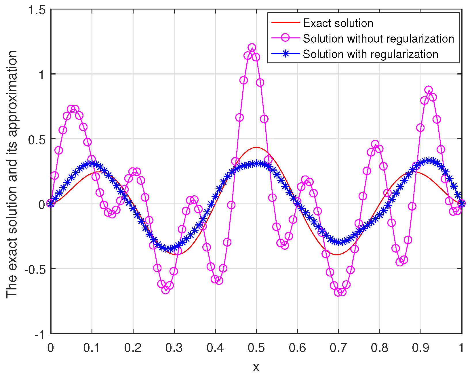
In Figure 1, we show the exact solution, the approximation solution without regularization, and the regularized solution for Example 1.

In Figure 2, we show the comparisons between the exact solution and its regularized solution for various noise levels $ϵ=0.00001$ and $ϵ=0.0001$ with $q=0.8$ in the case of $\alpha =0.8$.

Figure 3 illustrates the comparisons between the exact solution and its regularized solution for $q=1,q=0.8,q=0.5$ with $ϵ=0.00001$ in the case of $\alpha =0.8$.

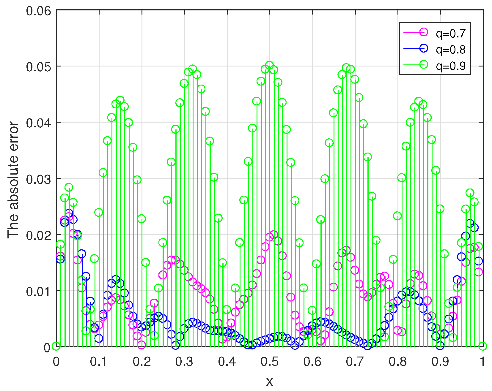
In Figure 4, the comparison of the absolute error between the exact solution and its regularized solution for $q=0.6,q=0.7,q=0.8$ with $ϵ=0.00001$ in the case of $\alpha =0.6$ is shown.

Example 2.

Consider a piecewise smooth function

$$f\left(x\right)=\left\{\begin{array}{cc}0,\hfill & 0\le x\le {\displaystyle \frac{1}{4}},\hfill \\ 4(x-{\displaystyle \frac{1}{4}}),\hfill & {\displaystyle \frac{1}{4}}<x\le {\displaystyle \frac{1}{2}},\hfill \\ -4(x-{\displaystyle \frac{3}{4}}),\hfill & {\displaystyle \frac{1}{2}}<x\le {\displaystyle \frac{3}{4}},\hfill \\ 0,\hfill & {\displaystyle \frac{3}{4}}<x\le 1.\hfill \end{array}\right.$$

(56)

In Figure 5, we show the comparisons between the exact solution and its regularized solution for various noise levels $ϵ=0.00001$ and $ϵ=0.0001$ with $q=0.8$ in the case of $\alpha =0.8$.

Figure 6 illustrates the comparisons between the exact solution and its regularized solution for $q=1,q=0.8,q=0.5$ with $ϵ=0.00001$ in the case of $\alpha =0.8$.

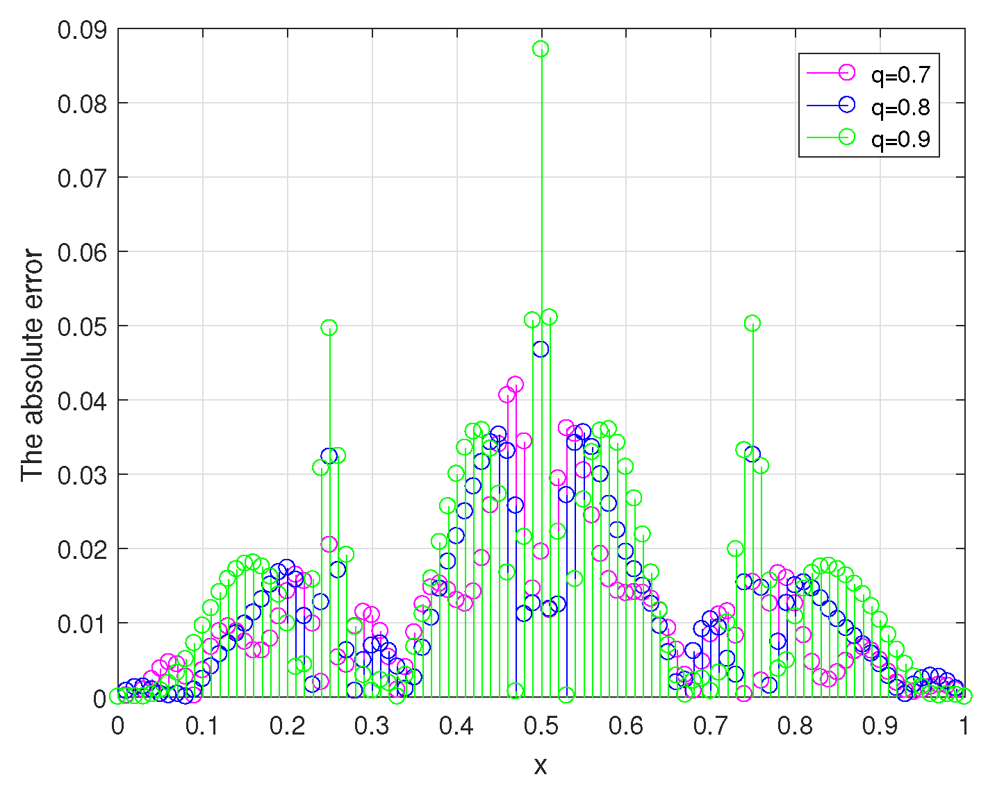
In Figure 7, the comparison of the absolute error between the exact solution and its regularized solution for $q=0.6,q=0.7,q=0.8$ with $ϵ=0.00001$ in the case of $\alpha =0.6$ is shown.

Example 3.

Consider a non-smooth function

$$f\left(x\right)=\left\{\begin{array}{cc}0,\hfill & 0\le x\le {\displaystyle \frac{1}{5}},\hfill \\ 1,\hfill & {\displaystyle \frac{1}{5}}<x\le {\displaystyle \frac{4}{5}},\hfill \\ 0,\hfill & {\displaystyle \frac{4}{5}}<x\le 1.\hfill \end{array}\right.$$

(57)

In Figure 8, we show the comparisons between the exact solution and its regularized solution for various noise levels $ϵ=0.00001$ and $ϵ=0.0001$ with $q=0.8$ in the case of $\alpha =0.8$.

Figure 9 illustrates the comparisons between the exact solution and its regularized solution for $q=1,q=0.8,q=0.5$ with $ϵ=0.00001$ in the case of $\alpha =0.8$.

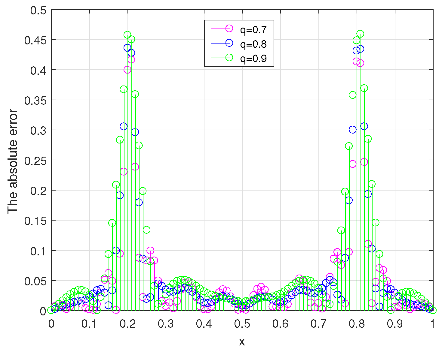
In Figure 10, the comparison of the absolute error between the exact solution and its regularized solution for $q=0.6,q=0.7,q=0.8$ with $ϵ=0.00001$ in the case of $\alpha =0.6$ is shown.

From a numerical perspective, we can draw four conclusions:

• Figure 1 shows us that the inverse space-dependent source problem (2) is ill-posed, and a stable approximate solution can be obtained by using the fractional Tikhonov regularization method.
• From Figure 2, Figure 5 and Figure 8, we know that the smaller the parameter $ϵ$ is, the better the computed approximation is.
• Figure 3, Figure 6 and Figure 9 show that the fractional regularization method ( ${\displaystyle \frac{1}{2}}<q<1$), Tikhonov regularization method ( $q=1$), and filter regularization method ( $q={\displaystyle \frac{1}{2}}$) are stable and effective. However, the Tikhonov regularization method obtains a smoother approximate solution; the fractional Tikhonov regularization method recovers the non-smooth points more accurately, and the filter regularization method can achieve good results for both smooth and non-smooth solutions.
• From Figure 4, Figure 7 and Figure 10, we find that for a fixed fractional order $\alpha$, in order to achieve better regularization results, we need to select the value of the parameter q appropriately, but the relationship between the two parameters needs further research.

5. Conclusions and Future Work

In this paper, we solve an inverse source problem for a Rayleigh–Stokes equation by using a fractional Tikhonov regularization method. Then, we prove the convergence rates under a priori and a posteriori regularization parameter selection rules, respectively. Finally, several numerical examples are given to illustrate the effectiveness of this method.

In the future, we will consider some numerical examples in higher-dimensional situations from a numerical perspective and also apply the other regularization techniques to solve this inverse source problem.

References

1. Podlubny, I. Fractional Diffusion Equation; Academic Press: New York, NY, USA, 1999. [Google Scholar]
2. Shen, F.; Tan, W.; Zhao, Y.; Masuoka, T. The Rayleigh-Stokes problem for a heated generalized second grade fluid with fractional derivative model. Nonlinear Anal. Real World Appl. 2006, 7, 1072–1080. [Google Scholar] [CrossRef]
3. Bazhlekova, E.; Lazarov, B.J.R.; Zhou, Z. An analysis of the Rayleigh-Stokes problem for a generalized second-grade fluid. Numerische Mathematik 2015, 132, 1–31. [Google Scholar] [CrossRef] [PubMed]
4. Khan, M. The Rayleigh-Stokes problem for an edge in a viscoelastic fluid with a fractional derivative model. Nonlinear Anal. Real World Appl. 2009, 10, 3190–3195. [Google Scholar] [CrossRef]
5. Zaky, M.A. An improved tau method for the multi-dimensional fractional Rayleigh-Stokes problem for a heated generalized second grade fluid. Comput. Math. Appl. 2018, 75, 2243–2258. [Google Scholar] [CrossRef]
6. Chen, C.M.; Liu, F.; Anh, V. Numerical analysis of the Rayleigh-Stokes problem for a heated generalized second grade fluid with fractional derivatives. Appl. Math. Comput. 2008, 204, 340–351. [Google Scholar] [CrossRef]
7. Chen, C.M.; Liu, F.; Burrage, K.; Chen, Y. Numerical methods of the variable-order Rayleigh-Stokes problem for a heated generalized second grade fluid with fractional derivative. IMA J. Appl. Math. 2013, 78, 924–944. [Google Scholar] [CrossRef]
8. Dehghan, M.; Abbaszadeh, M. A finite element method for the numerical solution of Rayleigh-Stokes problem for a heated generalized second grade fluid with fractional derivatives. Eng. Comput. 2017, 33, 587–605. [Google Scholar] [CrossRef]
9. Guan, Z.; Wang, X.D.; Ouyang, J. An improved finite difference/finite element method for the fractional Rayleigh-Stokes problem with a nonlinear source term. J. Appl. Math. Comput. 2021, 65, 451–479. [Google Scholar] [CrossRef]
10. Hadamard, J. Lectures on the Cauchy Problem in Linear Differential Equations; Yale University Press: New Haven, CT, USA, 1923. [Google Scholar]
11. Liu, S. Filter regularization method for inverse source problem of the Rayleigh-Stokes equation. Taiwan. J. Math. 2023, 27, 847–861. [Google Scholar] [CrossRef]
12. Binh, T.T.; Nashine, H.K.; Long, L.D.; Luc, N.H.; Nguyen, C. Identification of source term for the ill-posed Rayleigh-Stokes problem by Tikhonov regularization method. Adv. Differ. Equations 2019, 2019, 331. [Google Scholar] [CrossRef]
13. Klann, E.; Ramlau, R. Regularization by fractional filter methods and data smoothing. Inverse Probl. 2008, 24, 025018. [Google Scholar] [CrossRef]
14. Gerth, D.; Klann, E.; Ramlau, R.; Reichel, L. On fractional Tikhonov regularization. J. Inverse Ill-Posed Probl. 2015, 23, 611–625. [Google Scholar] [CrossRef]
15. Xiong, X.T.; Xue, X. A fractional Tikhonov regularization method for identifying a space-dependent source in the time-fractional diffusion equation. Appl. Math. Comput. 2019, 349, 292–303. [Google Scholar] [CrossRef]
16. Yang, F.; Pu, Q.; Li, X.X. The fractional Tikhonov regularization methods for identifying the initial value problem for a time-fractional diffusion equation. J. Comput. Appl. Math. 2020, 380, 112998. [Google Scholar] [CrossRef]
17. Zheng, G.H.; Zhang, Q.G. Solving the backward problem for space-fractional diffusion equation by a fractional Tikhonov regularization method. Math. Comput. Simul. 2018, 148, 37–47. [Google Scholar] [CrossRef]
18. Djennadi, S.; Shawagfeh, N.; Arqub, O.A. A fractional Tikhonov regularization method for an inverse backward and source problems in the time-space fractional diffusion equations. Chaos Solitons Fractals 2021, 150, 111127. [Google Scholar] [CrossRef]
19. Qian, Z.; Feng, X.L. A fractional Tikhonov method for solving a Cauchy problem of Helmholtz equation. Appl. Anal. 2017, 96, 1656–1668. [Google Scholar] [CrossRef]
20. Duc, P.N.; Binh, H.D.; Long, L.D.; Van, H.T.K. Reconstructing the right-hand side of the Rayleigh-Stokes problem with nonlocal in time condition. Adv. Differ. Equations 2021, 2021, 470. [Google Scholar] [CrossRef]
21. Xiong, X.T.; Xue, X.M. Fractional Tikhonov method for an inverse time-fractional diffusion problem in 2-dimensional space. Bull. Malays. Math. Sci. Soc. 2020, 43, 25–38. [Google Scholar] [CrossRef]
22. Yang, F.; Cao, Y.; Li, X.X. Two regularization methods for identifying the source term of Caputo-Hadamard time-fractional diffusion equation. Math. Methods Appl. Sci. 2023, 46, 16170–16202. [Google Scholar] [CrossRef]
23. Nguyen, A.T.; Luu, V.C.H.; Nguyen, H.L.; Nguyen, H.T.; Nguyen, V.T. Identification of source term for the Rayleigh-Stokes problem with Gaussian random noise. Math. Methods Appl. Sci. 2018, 41, 5593–5601. [Google Scholar] [CrossRef]
24. Kirsch, A. An Introduction to the Mathematical Theory of Inverse Problems, 2nd ed.; Volume 120 of Applied Mathematical Sciences; Springer: New York, NY, USA, 2011. [Google Scholar]
25. Wu, C. Numerical solution for Stokes’ first problem for a heated generalized second grade fluid with fractional derivative. Appl. Numer. Math. 2009, 59, 2571–2583. [Google Scholar] [CrossRef]
Figure 1. A comparison of the exact solution, the approximation solution without regularization and the approximation solution with regularization for q = 0.95 , α = 0.6 with ϵ = 0.001 for Example 1.
Fractalfract 08 00601 g001
Figure 2. A comparison between f and f μ , q δ for different noisy levels with q = 0.8 at α = 0.8 for Example 1, (a) the exact solution and its approximation, (b) the absolute error.
Fractalfract 08 00601 g002
Figure 3. A comparison between f and f μ , q δ for different values of q with ϵ = 0.00001 at α = 0.8 for Example 1, (a) the exact solution and its approximation, (b) the absolute error.
Fractalfract 08 00601 g003
Figure 4. A comparison of the absolute error between f and f μ , q δ for different values of q with ϵ = 0.00001 and α = 0.6 for Example 1.
Fractalfract 08 00601 g004
Figure 5. A comparison between f and f μ , q δ for different noisy levels with q = 0.8 at α = 0.8 for Example 2, (a) the exact solution and its approximation, (b) the absolute error.
Fractalfract 08 00601 g005
Figure 6. A comparison between f and f μ , q δ for different values of q with ϵ = 0.00001 at α = 0.8 for Example 2, (a) the exact solution and its approximation, (b) the absolute error.
Fractalfract 08 00601 g006
Figure 7. A comparison of the absolute error between f and f μ , q δ for different values of q with ϵ = 0.00001 and α = 0.6 for Example 2.
Fractalfract 08 00601 g007
Figure 8. A comparison between f and f μ , q δ for different noisy levels with q = 0.8 at α = 0.8 for Example 3, (a) the exact solution and its approximation, (b) the absolute error.
Fractalfract 08 00601 g008
Figure 9. A comparison between f and f μ , q δ for different values of q with ϵ = 0.00001 at α = 0.8 for Example 3, (a) the exact solution and its approximation, (b) the absolute error.
Fractalfract 08 00601 g009
Figure 10. A comparison of the absolute error between f and f μ , q δ for different values of q with ϵ = 0.00001 and α = 0.6 for Example 3.
Fractalfract 08 00601 g010
Disclaimer/Publisher’s Note: The statements, opinions and data contained in all publications are solely those of the individual author(s) and contributor(s) and not of MDPI and/or the editor(s). MDPI and/or the editor(s) disclaim responsibility for any injury to people or property resulting from any ideas, methods, instructions or products referred to in the content.