Unsupervised Machine Learning-Based Singularity Models: A Case Study of the Taiwan Strait Basin

Abstract

The identification of geochemical anomalies in oil and gas indicators is a fundamental task in oil and gas exploration, as the process of oil and gas accumulation is a low probability event. Machine learning algorithms for anomaly detection are applicable to the identification of oil and gas geochemical anomalies related to oil and gas accumulation. However, when using oil and gas indicators for anomaly detection, the diversity of these indicators often leads to the influence of the indicator redundancy on the identification of such features. Therefore, it is particularly important to select appropriate oil and gas indicators for anomaly detection. In this study, a hybrid model combining unsupervised machine learning methods and singularity analysis methods was used to evaluate oil and gas indicator anomalies using geochemical data from the Taiwan Strait Basin. The models used in this study include the singularity index model, the principal component model combined with the singularity index model, and the cluster analysis combined with the principal component model and the singularity index model. PCA models can reduce the dimensions of the data and retain as much information as possible. CLA divides data samples into different groups, so that samples within the same group are more similar and samples between different groups are less similar. LSP is mainly used for measuring the setting and singular degree of local anomalies in multi-scale geochemistry, geophysics, and other types of local anomalies, and it has a unique advantage in extracting low and weak anomalies and nonlinear characteristics. The results of the study show that the results obtained using the CLA-PCA-LSP hybrid model are very similar to those obtained by performing PCA on the entire index and then calculating the singularity index. This also verifies that, for the study areas of the Jiulongjiang Depression and Jinjiang Depression, we can select oil and gas indicators that are favorable for exploration analysis, without including all indicators in the analysis scope, thereby improving the computational efficiency. The application of a singularity analysis method and generalized self-similarity principle in extracting the geochemical information of oil and gas indicators in the Taiwan Strait Basin highlights key technologies such as the identification of weak anomalies, decomposition of composite anomalies, and integration of spatial information. The combination anomalies delineated by the singularity analysis method and S-A method not only reflect the spatial relationship with known oil and gas reservoir distribution, but also show the multiple combination anomalies in unknown areas, providing favorable guidance for the next exploration direction in the Taiwan Strait Basin.

1. Introduction

The growing global demand for mineral resources necessitates that exploration efforts maintain or enhance the rate of discovery of mineral deposits [1,2,3], presenting numerous challenges to exploration activities. One such challenge is how to effectively integrate diverse datasets, including geochemical, geophysical, and geological structural data, for conducting prospecting surveys [4,5,6,7,8,9]. This endeavor necessitates interdisciplinary collaboration and the application of mathematical techniques. Subsequently, various statistical methods have been developed to address professional challenges across different fields. These include fractal and multifractal models [10], univariate analysis [11], multivariate analysis [12], and geostatistics [13]. So, which method is suitable for which data is also a problem we need to discuss, which often needs experts to prove through practice, so that the method we choose can reflect the problem we need to solve as much as possible.

The extensive data generated by geological studies encompass not only qualitative and quantitative data but also textual descriptions, geological videos, and more. The challenge lies in efficiently utilizing these data to enhance mineral exploration, an issue at the intersection of big data and geology. We propose that the integration of geology with data science can be achieved through cloud platforms, leveraging GIS spatiotemporal data models, and dynamically managing geological spatiotemporal big data models. Furthermore, we underscore the necessity of interdisciplinary collaboration by employing a range of data methodologies to address modeling challenges in geology, incorporating cloud computing and artificial intelligence into the analysis of geological big data to inform geological exploration.

In recent decades, multifractal methods have become a popular approach for locating geochemical anomalies. Among them, the C-A fractal method has been widely used in mineral prediction [10], which is particularly useful for identifying geochemical anomalies. For the identification of deeper-level anomalies, the S-A method and singularity analysis method have shown advantages [14,15]. It is well known that supervised machine learning methods rely on well-defined mineralization types with good features in different geological environments to label geochemical indicators and sample classifications. The prediction of uncertain areas using supervised machine learning methods, which utilize large amounts of data and information, can be challenging, especially in different geological environments with different features and background values. In contrast, unsupervised machine learning techniques, such as cluster analysis, do not require sample classifications but require expert validation to determine the number and meaning of clusters [16,17,18].

The purpose of this study is to incorporate multiple fractal singular results into the unsupervised learning algorithm of clustering principal components, in order to enhance the identification of abnormal geochemical indicators in the Taiwan Strait Basin. There are more than twenty geochemical indicators for oil and gas in the Taiwan Strait Basin. If we perform calculations on all indicators, it could lead to the incorporation of extensive and comprehensive data information. However, if there is redundant information in these data that may affect the calculation results, it is necessary to eliminate this useless information. In this study, unsupervised machine learning methods and comprehensive singularity analysis methods are used to identify abnormal geochemical indicators in the Taiwan Strait Basin. This strategy aims to identify unknown favorable areas that cannot be explained by the currently available surface indicators. The findings of this study strongly endorse the efficacy of abnormality detection in geochemical data and clustering principal component methods for mineral exploration in the Taiwan Strait Basin.

Oil and gas exploration in the Taiwan Strait Basin commenced in the late 20th century. Numerous organizations, including the Second Marine Geological Survey Brigade of the Ministry of Geology and Mineral Resources, the Guangzhou Marine Geological Survey Bureau, the State Oceanic Administration, the Chinese Academy of Geological Sciences, and various domestic and foreign oil companies, have conducted exploration activities in the region utilizing a range of techniques, such as gravity, magnetic, electrical, seismic, and geochemical surveys, leading to significant exploration accomplishments. The Guangzhou Marine Geological Survey Bureau has carried out extensive fundamental research in the area. The results from gravity, magnetic, seismic, and geological studies have identified three sets of promising hydrocarbon source rock series in the Taiwan Strait Basin, namely the Paleogene, Eocene, and Miocene. The reservoirs primarily comprise Paleogene and Eocene tidal sandstones, while the regional cap rocks are made up of Miocene and Quaternary mudstones. Previous studies on the Taiwan Strait Basin have predominantly focused on the tectonic and sedimentary evolution, with less emphasis on utilizing oil and gas indicators for prospecting analysis. This article presents a novel approach utilizing unsupervised machine learning-based singularity patterns to identify local variability and spatial structural information of anomalies in the Taiwan Strait Basin. The method, which combines spatial statistical analysis and singularity assessment, not only accounts for the spatial correlation and variability of field values but also effectively captures the local singularity of the field. This technique is employed to analyze geochemical data related to oil and gas indicators in the Taiwan Strait Basin, aiming to delineate the comprehensive anomaly zones of these indicators. The results offer valuable insights for oil and gas exploration and evaluation in the region. Conducting geochemical exploration for oil and gas in the Taiwan Strait Basin and investigating the response characteristics and distribution patterns of oil and gas indicators can provide direct evidence indicating the presence of deep oil and gas reservoirs. Geophysical and petroleum geological studies suggest that the Taiwan Strait possesses significant oil and gas potential, with oil and gas flows identified in the Jiulong River depression. To further assess the hydrocarbon potential of other structures, it is essential to conduct geochemical anomaly analyses to obtain direct evidence of oil and gas presence. Currently, CNOOC has undertaken drilling activities in the central and southern regions of the Taiwan Strait, leading to the discovery of several gas fields in the eastern area. These findings validate our analysis of the region and will support our future exploration efforts. In this study, we constructed the singularity pattern (LSP) based on unsupervised machine learning, as well as the hybrid models (PCA-LSP, CLA-PCA-LSP) that combine the singularity model with dimensionality reduction techniques. The effectiveness of these models in identifying geochemical anomalies in multiple indicators in the Taiwan Strait Basin was evaluated. These models include: (1) singularity index model; (2) the extraction of components and deep features of original indicator data using PCA and singularity index dimensionality reduction methods, respectively; (3) the selection of variables in the indicator dataset using the CLA method and the extraction of components and deep features of the indicator dataset using PCA and LSP, respectively.

Previous studies on the Taiwan Strait have primarily concentrated on fundamental basin analyses, employing traditional statistical methods to delineate anomalies. In contrast, this study utilizes unsupervised machine learning and singularity analysis to examine the Taiwan Strait, allowing for the identification of low, gentle, and weak anomaly areas that traditional methodologies cannot reveal. The significance of these identified anomaly areas has been corroborated through subsequent geophysical analyses.

2. Study Area and Data

2.1. Geological Setting

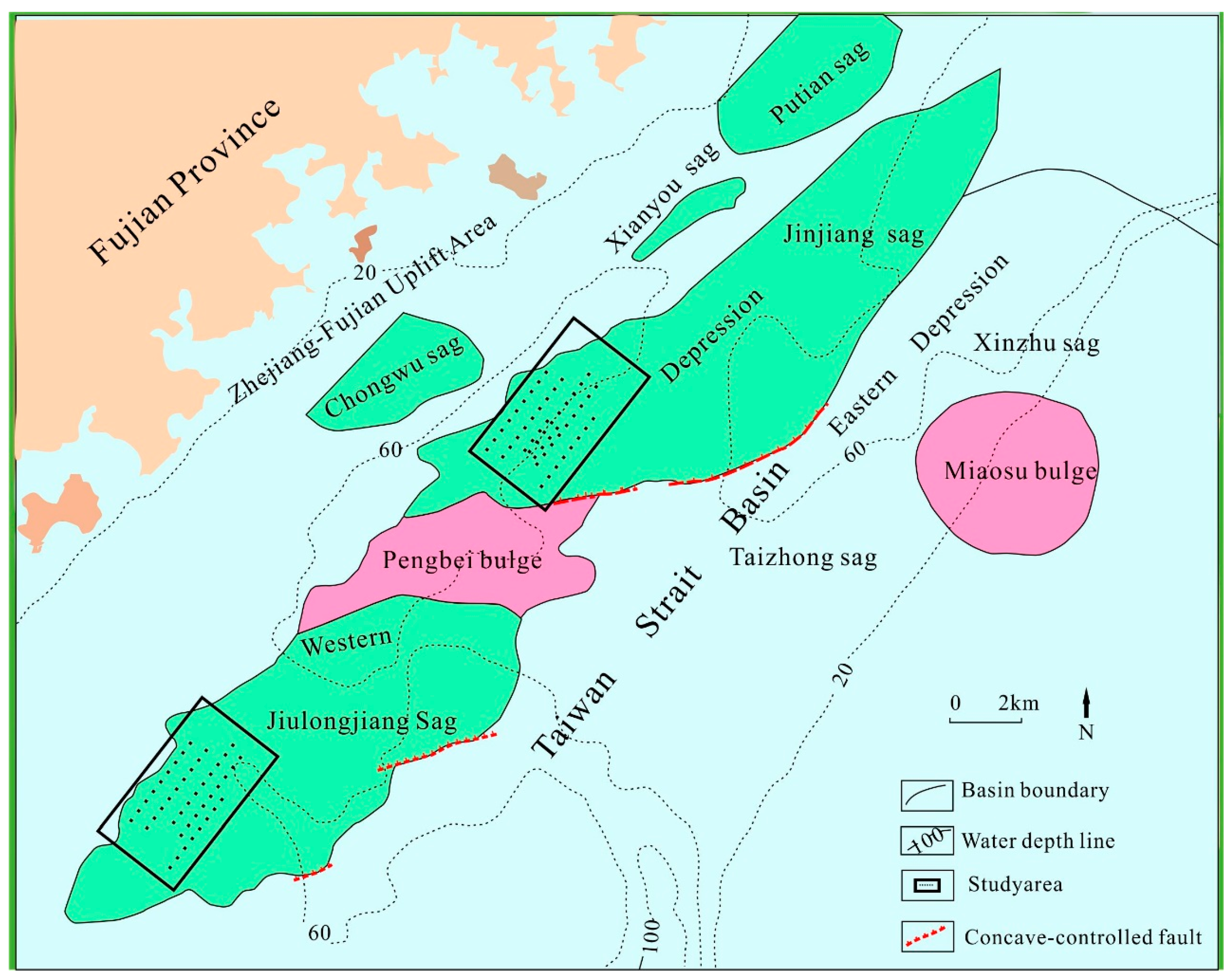
The Taiwan Strait Basin is a Cenozoic continental margin rift basin that developed within an intracontinental extensional setting. Subsequently, it became superimposed on a foreland basin and displays a structural configuration characterized by four depressions and two uplifts: the Jinjiang Depression, Hsinchu Depression, Jiulongjiang Depression, Taichung Depression, Pengbei Uplift, and Miaoli Uplift. The basin is intersected by three sets of faults oriented northeast (NE), northwest (NW), and nearly south–north (SN) (see Figure 1). The western section of the Taiwan Strait Basin, known as the Taixi Basin, is situated in the northern part of the Taiwan Strait, with its western boundary defined by the coastal fault zone located east of the Zhejiang–Fujian Uplift. The eastern boundary is marked by the Quchi-Laocong Fault, which lies west of the Central Mountain Range in Taiwan. To the north, the basin is bordered by the Guanyin Uplift, separating it from the East China Sea Shelf, while to the south, it is delineated by the Penghu–Beigang Uplift, which separates it from the Pearl River Mouth Basin and the southwestern Taiwan Basin. The Taiwan Strait Basin encompasses an area of approximately 39,000 km².

The Jinjiang Depression is a narrow and elongated half-graben with east-dipping and west-overlapping faults. The strata thicken from west to east, and the sediment source is mainly from the west side of the Min-Zhe Uplift, transported from west to east. The sediment on the west side is coarser, while the sediment near the depositional center on the east side is finer. Therefore, the better reservoir rocks should be on the west side, while the source rocks should be on the east side. According to the analysis [19] of the basin’s evolution and sedimentary patterns, there are shale deposits from the Paleogene syn-rift period, including lake and fan-delta sediments. These shales should be rich in organic matter due to the semi-closed environment, making them good source rocks for oil generation. The deep depression zone on the eastern margin of the basin is the oil generation center. Preliminary geochemical maturity simulations show that the Paleogene source rocks in the central part of the basin entered the mature stage in the Eocene, and the generated oil and gas can be accumulated in the sand layers of the Paleogene, with the shale of the Eocene as the main cap rock. Therefore, the Paleogene is the most prospective formation for oil and gas accumulation in this basin. Although the lower Eocene is mainly shale, the thin sand layers within it may also contain oil and gas [20].

The Jinjiang Depression and Jiulongjiang Depression have similar petroleum geological conditions. In the central part of the Jiulongjiang Depression, lacustrine deposits of the Eocene/Oligocene have been encountered, and it is also possible that the Paleogene strata in the Jinjiang Depression contain good quality lacustrine source rocks. Based on seismic facies analysis, the Eocene formations are interpreted to represent delta plain to delta front environments, which may also contain fair to good quality source rocks [19].

2.2. Geochemical Data

The data presented in this study were collected from the Jiulongjiang Depression and Jinjiang Depression within the Taiwan Strait Basin. The indicators utilized in the analysis include acid-extractable hydrocarbons, thermally released hydrocarbons, total aromatic hydrocarbons and their derivatives, weathered carbonates, and microorganisms. Acid-extractable hydrocarbons were analyzed using an Agilent 7890A gas chromatograph (Agilent Technologies, Santa Clara, CA, USA), employing the GBW(E)061164 nitrogen-based C1-C5 mixed gas standard for calibration. The results are expressed as the volume of each hydrocarbon component per unit mass of the sample, in μL/kg. The thermally released hydrocarbons were also analyzed using an Agilent 7890A gas chromatograph from Agilent Technologies, USA, with GBW(E)061164 nitrogen-based C1-C5 mixed gas standard substance. The results are expressed as the volume of each hydrocarbon component per unit mass of the sample, in μL/kg. The weathered carbonates were analyzed using a GXH-1050 infrared gas analyzer from Beijing Jufang Physical and Chemical Technology Research Institute (Beijing, China), with two high-precision temperature-controlled furnaces as auxiliary instruments, and GBW(E)0060856 nitrogen-based carbon dioxide gas standard substance. The main measurement was the volume percentage of carbon dioxide in the decomposed gas of the sample at 500–600 °C, which was used to measure the content of weathered carbonate components in the sample. ΔC represents weathered carbonates, with units of 10⁻². The total amount of aromatic hydrocarbons and polycyclic aromatic hydrocarbons was analyzed using an LS55 fluorescence spectrophotometer from PE Corporation, Boston, MA, USA, with spectroscopically pure naphthalene as the standard substance. This measurement was mainly used to quantify the content of polycyclic aromatic hydrocarbons in the sample, with units of 10⁻⁶. The sediment soil samples for oil and gas microbiological detection were collected at a depth of 20 cm underwater. After being frozen and stored, they were transported to the laboratory for analysis. The MV value represents the abundance of original hydrocarbon microorganisms.

The indicators used in the study include: Acidolysis hydrocarbon methane (ACH₄), Acidolysis hydrocarbon ethane (AC₂H₆), Acidolysis hydrocarbon ethylene (AC₂H₄), Acidolysis hydrocarbon propane (AC₃H₈), Acidolysis hydrocarbon isobutane (ACH₃CH(CH₃)CH₃), Acidolysis hydrocarbon propylene (AC₃H₆), Acidolysis hydrocarbon n-butane (ACH₃CH₂CH₂CH₃), Total polycyclic aromatic hydrocarbons 320 nm (320 nmF320), Total polycyclic aromatic hydrocarbons 360 nm (360 nmF360), Total polycyclic aromatic hydrocarbons 405 nm (405 nmF405), Pyrolyzed hydrocarbon methane (PCH₄), Pyrolyzed hydrocarbon ethane (PC₂H₆), Pyrolyzed hydrocarbon ethylene (PC₂H₄), Pyrolyzed hydrocarbon propylene (PC₃H₆), Pyrolyzed hydrocarbon propane (PC₃H₈), Pyrolyzed hydrocarbon isobutane (PCH₃CH(CH₃)CH₃), Pyrolyzed hydrocarbon isopentane (PCH₃CH₂CH(CH₃)CH₃), Pyrolyzed hydrocarbon n-butane (PCH₃CH₂CH₂CH₃), Pyrolyzed hydrocarbon n-pentane (PCH₃CH₂CH₂CH₃), Erosion carbonate (ΔC), MV (exclusive hydrocarbon oxidizing bacteria content), and Total aromatics and their derivatives 260 nm (UV260).

3. Methods

3.1. S-A

The S-A model is characterized by a power–law relationship expressed as:

A(>S)∝S^−β

where S represents the energy spectral density. When the energy spectral density is set to a critical value S₀, A denotes the area where S > S₀.

By taking the logarithm of the aforementioned equation, we applied the least squares method to fit the relationship between (log A) and (log S) in a piecewise manner to determine the power index β across various spectral density ranges. In the (log A)–(log S) plot, all linear segments conform to the power–law relationship. Each segment corresponds to a distinct fractal relationship, with different segments representing varying fractal characteristics. The x-coordinate value at the intersection of each segment defines the threshold value for the fractal filter. Utilizing these thresholds, we are able to construct the background and anomaly filters, thereby facilitating the separation of background and anomalies by transforming them into the spatial domain using these filters.

3.2. LSP

The developed method of local singularity analysis can be used to delineate and quantify the degree of singularity of multiscale geochemical, geophysical, and other types of local anomalies. The principle is to decompose the field values defined within a small range into two components based on the scale scaling of the field ($<\mathsf{\rho }\left(\mathsf{\epsilon }\right)>=\mathrm{c}{\epsilon }^{\alpha -2}=c{\epsilon }^{-∆\alpha }$) [21]. There are two components related to the measurement scale unit of density (c) (such as units of g/$m^{\alpha }$): one is the scale component $∆\alpha$ independent of the measurement scale unit, and the other is the density component with density characteristics. The measurement unit can be g/${cm}^{1.5}$, which can be called fractal density [22]. The exponent α in the latter corresponds to the fractal dimension of space. The method of local singularity analysis actually measures the intensity or density of the field in fractal space to determine the fractal density c and the fractal dimension α. The difference between the fractal dimension and the normal Euclidean dimension $∆\alpha =2-\alpha$ (for two-dimensional fields) represents the difference in spatial dimension between fractal density and normal density. When $∆\alpha$ is not an integer, the density is called fractal density, and as the measurement range decreases, such as when ε approaches 0, the density becomes infinitely large or infinitely small. When the density belongs to fractal density and $∆\alpha =2-\alpha >0$, as the measurement range decreases, such as when ε approaches 0, the density becomes infinitely large and exhibits nonlinear singular characteristics such as non-smoothness, instability, and non-convergence at that position. Conversely, when the density belongs to fractal density and $∆\alpha =2-\alpha <0$, as the measurement range decreases, such as when ε approaches 0, the density of the field approaches 0 and exhibits nonlinear singular characteristics such as high-order derivative non-existence, non-smoothness, instability, and non-convergence at that position. Only when $∆\alpha =2-\alpha \cong 0$, the density is independent of the size of the measurement range. From the perspective of geochemical fields, regions with positive singularity ($∆\alpha >0$) correspond to enrichment areas of elements, while regions with negative singularity ($∆\alpha <0$) correspond to depletion areas of elements. Regions without singularity correspond to background fields, which generally occupy the majority of the range [21,23].

In a two-dimensional environment, the model for local singularity analysis is defined as follows:

u = cA^α/2

C(A) = cA^(α/2)−1

In the equation above, c represents a constant, while α denotes the singularity index. The calculation process for the singularity index is as follows:

First, we define a set of rectangular windows of size e centered on the sample point. Next, we plot the concentration of the indicator against the window size e across all rectangular windows C(e) using a double logarithmic scale. Subsequently, we apply the least squares method to fit the data and determine the slope k of the double logarithmic plot, which is used to estimate the singularity index α, defined as (k + 2). Finally, by repeating these steps for all sample positions, we can obtain the spatial distribution of the singularity index.

LogC[A(e_i)] = c + (α-2)/log(e_i)

3.3. PCA-LSP

Principal component analysis (PCA) is a widely utilized technique for dimensionality reduction that effectively retains the essential information and structure of data within a lower-dimensional space [24,25]. The primary objective of PCA is to transform a set of originally correlated variables (e.g., P indicators) into a new set of uncorrelated composite indicators. This transformation is accomplished through the linear combination of the original P indicators to generate new composite indicators.

In this context, the variance of the first linear combination, denoted as Var(F1), is of particular interest. A greater Var(F1) signifies that the first principal component, F1, encapsulates more information. Consequently, F1 is selected as the linear combination that exhibits the highest variance. If F1 does not sufficiently represent the information contained in the original P indicators, the analysis proceeds to consider the second linear combination, F2. To ensure that F2 effectively captures distinct information, it is essential that the information represented by F1 does not overlap with that of F2. This requirement is mathematically expressed as Cov(F1, F2) = 0, with F2 being designated as the second principal component. This iterative process can be continued to derive additional principal components, including the third, fourth, and up to the Pth component. By combining PCA with singularity analysis, a joint model called PCA-LSP is established. In this study, a new method is proposed where PCA is applied to the original data first, followed by singularity analysis, with the aim of extracting comprehensive abnormal information from the indicators.

The covariance matrix is constructed from the covariances of multiple random variables. Let the dataset consist of n samples, each containing d features, which can be represented as an n times d matrix X. If the mean of each feature is denoted as u, the covariance matrix E can be calculated using the following formula:

E = (X − u)(X − u)^T/n

where (X − u) represents the centering of each sample by subtracting the mean u. Consequently, each element of the covariance matrix corresponds to the covariance between the respective features.

3.4. CLA-PCA-LSP

Cluster analysis (CLA) has proven effective in extracting and distinguishing elements closely associated with mineralization events [26,27,28,29]. The fundamental principle of CLA is to identify the internal structure and patterns within the dataset, thereby enhancing the understanding of its composition and characteristics. By iteratively grouping variables that exhibit high correlations, CLA can identify key indicator variables [26,28]. This method is classified as unsupervised learning, and the relationships between variables can be visualized using a dendrogram. Variables are assigned to distinct clusters based on an appropriate similarity threshold, which is typically determined by correlation coefficients.

In this study, we employed a hybrid approach that integrates cluster analysis, principal component analysis, and singularity analysis to identify anomalous characteristics of oil and gas indicators in the study area. Following the grouping obtained from cluster analysis, the principal component analysis was performed on the indicators to derive comprehensive results. Subsequently, the singularity analysis was utilized to define the range of combined anomalies. For the r-type clustering analysis of the indicators, we applied the (1—Pearson r) distance metric along with the complete linkage hierarchical clustering method.

4. Results and Discussion

4.1. Weak Anomaly Extraction and Delineation

4.1.1. Local Singularity Analysis and Local Anomaly Delineation

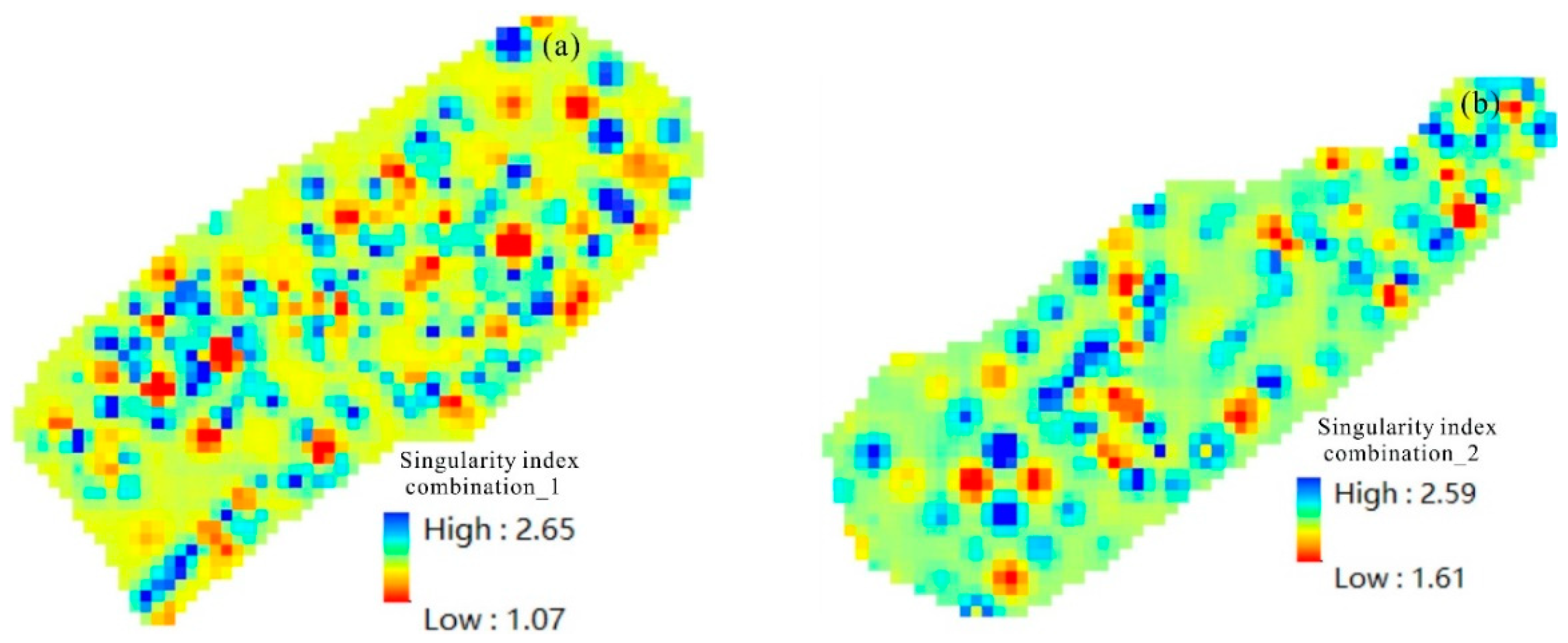
Compared to other types of geological anomalies, geochemical anomalies not only have a high numerical accuracy in their chemical analysis content, but also can reflect the multi-scale spatial variation patterns of anomalies more continuously. It can provide a more comprehensive reflection of the spatial structure of anomalies. Therefore, quantifying the local structural patterns of geochemical anomalies helps to understand the structure of anomalies and provides new clues for anomaly identification. This study found that geochemical anomalies are strong in the northwest and central parts of the Jiulong River Depression and the southwest part of the Jinjiang Depression, while in other areas, geochemical anomalies are masked and not clearly displayed. In order to enhance and highlight local anomalies, we calculated their singularity index. Taking thermal hydrocarbon propane as an example, the local singularity analysis method was used to highlight local anomalies and avoid the influence of background field values on anomaly delineation. When calculating the singularity index, different window sizes were formed on the geochemical map with each point as the center: 2 km × 2 km, 6 km × 6 km, 10 km × 10 km, 14 km × 14 km, …, 26 km × 26 km. The average index density within each window was calculated, and the relationship between average density and window size was plotted on a double logarithmic graph. Then, linear regression was performed on the data obtained from multiple windows using the least squares method, and the slope of the regression line was taken as the singularity index value Δα. The local singularity index map was formed by calculating the local singularity index at each point. Figure 2a shows the distribution map of the singularity index of the indicator thermal hydrocarbon propane. At the same time, we used the IDW method with a minimum of 12 sample points and a maximum search window of 26 km × 26 km to perform moving average on the original content data of the above indicators, as shown in Figure 2b. From the figure, it can be seen that the strong geochemical background in the southwest part of the Jinjiang Depression masks the weak and gradual anomalies that may exist in the southwest part. This also precisely illustrates the limitation of dividing background and anomalies based on content values. However, from the singularity index map in Figure 2a, the regions where Δα > 0 or α < 2 are correlated with the spatial distribution of oil and gas reservoirs in the study area, indicating that Δα > 0 or α < 2 can reflect the abnormal information of oil and gas indicator content.

Figure 3 presents a comparison of anomalies identified by the local singularity method and traditional statistical methods. The results indicate that both the singularity analysis method and the traditional method based on the element content are correlated with the spatial distribution of known favorable areas. However, the singularity method not only correlates with the distribution of favorable areas and oil and gas zones, but also identifies better anomalies in unknown areas, making it more predictive.

4.1.2. Local Singularity Analysis and Combined Local Anomaly Delineation

To delineate comprehensive anomalies using these oil and gas indicators, we conducted a principal component analysis (PCA) on the singular values (α values) of these indicators (Figure 4). The eigenvalues of the 19 principal components showed that the first principal component accounted for approximately 70% of the variance, indicating its significance. The results reveal that the first principal component was composed of all the indicators, and the resulting composite local singularity map (factor score map) clearly reflected the spatial anomaly patterns of the Jiulongjiang and Jinjiang Depressions. These anomalies were closely related to the intersection of faults, suggesting their potential control on oil and gas characteristics.

4.2. Decomposition and Delineation of Complex Anomalies

The S-A method quantifies the scale characteristics of the general scale invariance and spatial patterns of anisotropy exhibited by geochemical indicators. It not only separates isotropic anomalies caused by geological bodies at different depths, such as various geophysical fields, but also separates anisotropic anomalies caused by more complex geological processes.

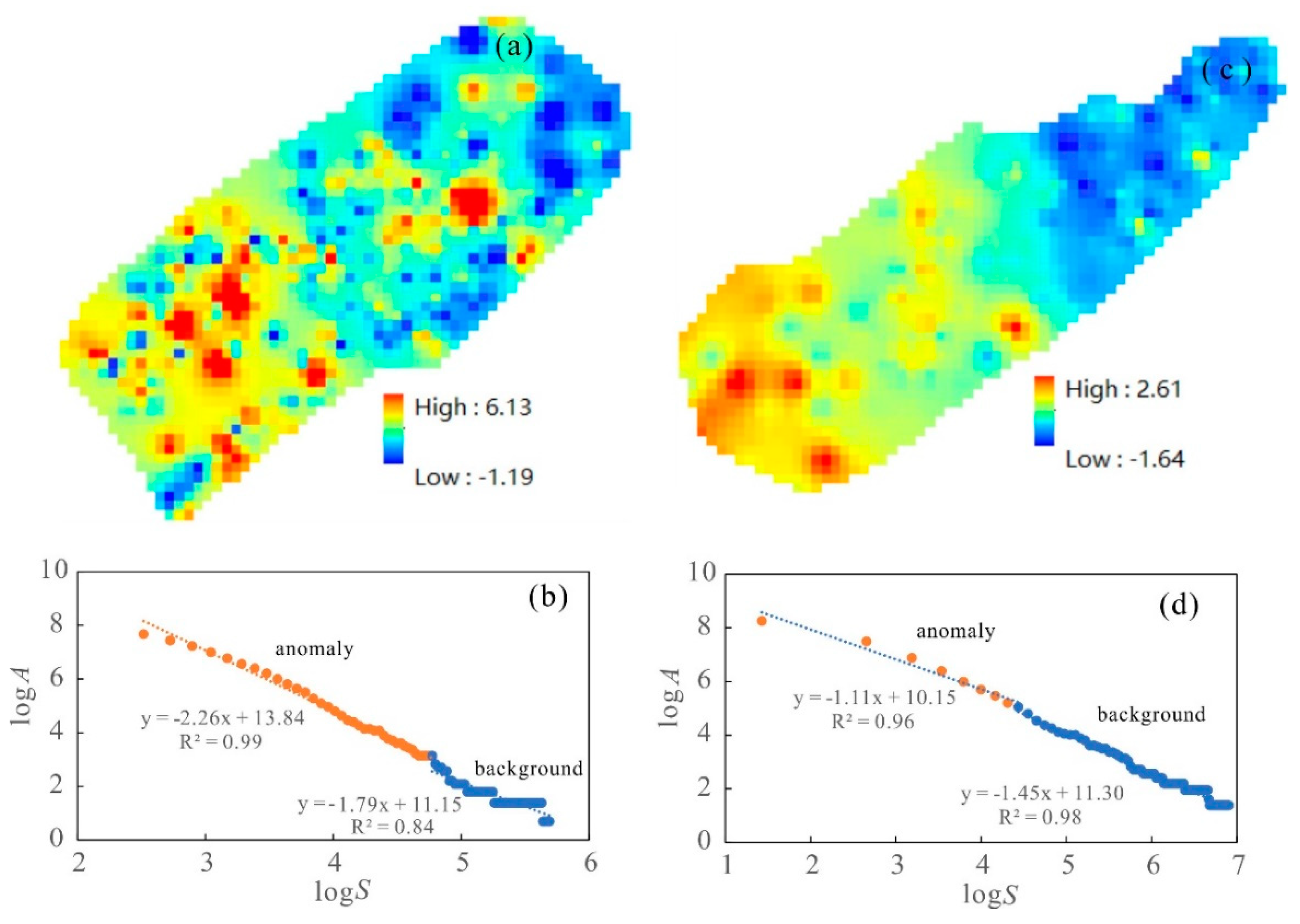
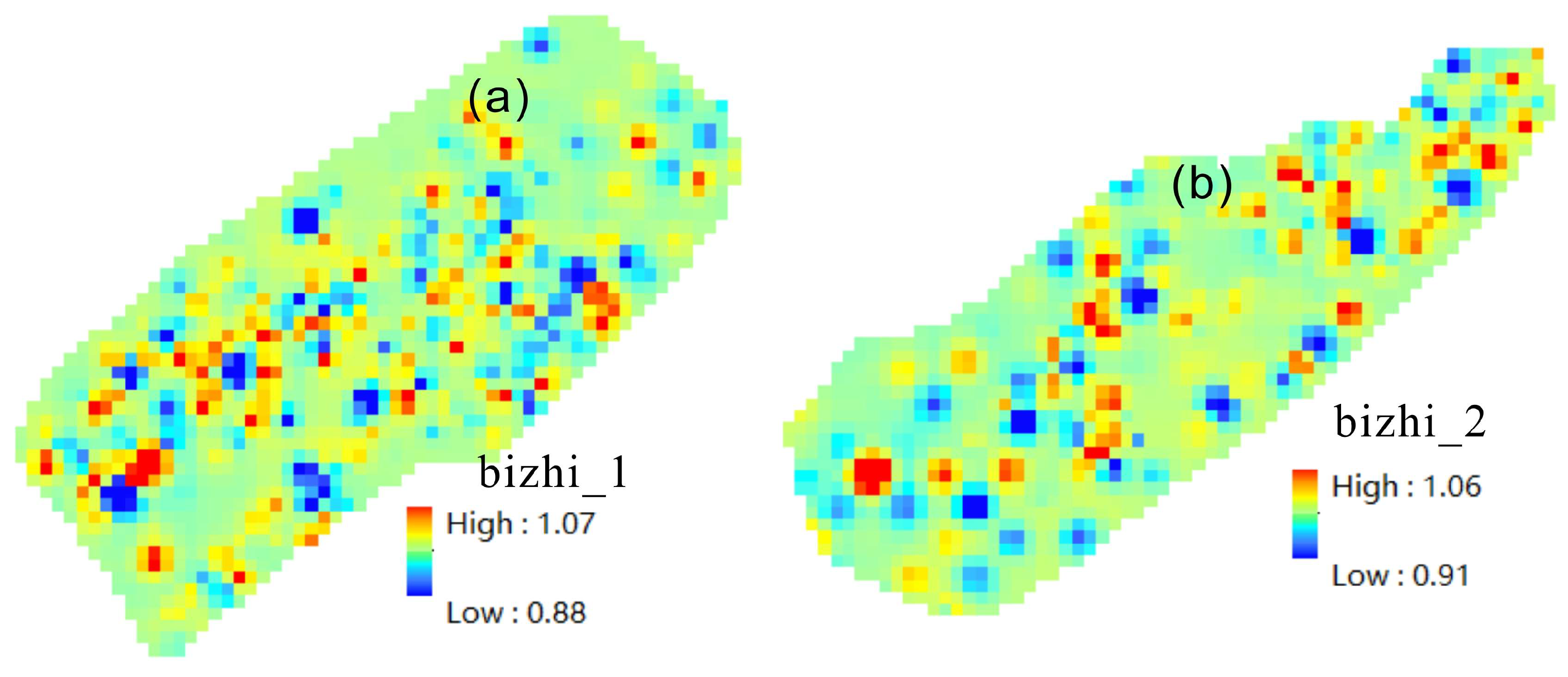
In this study, a principal component analysis (PCA) was first used to analyze the raw data of all indicators. Figure 5 shows the distribution of eigenvalues calculated by PCA and the loading plot of the first principal component. It can be observed that the first principal component reflects the common contribution of all indicators. Figure 6a,c show the score maps of the first principal component. The results indicate that high scores of the first principal component are located in the southwest of the Jiulongjiang and Jinjiang Depressions. Previous studies have shown that this area is adjacent to the hydrocarbon center [19]. For the Jiulongjiang Depression, there are excellent hydrocarbon source rocks in the Paleogene Lake facies, and multiple oil-source faults connect the hydrocarbon center, facilitating oil and gas accumulation. For the Jinjiang Depression, the southwest part is its hydrocarbon center, with two large east–west faults connecting the hydrocarbon center, providing favorable pathways.

For the Jiulongjiang Depression:

Using the S-A method (Cheng et al., 2000) [22], the combined original anomaly map in Figure 6a is first transformed into the frequency domain through Fourier transformation, resulting in phase distribution and power–spectrum distribution. Then, the relationship between spectral density (S) and cumulative area is plotted on a double logarithmic graph, as shown in Figure 6b. The relationship between spectral density (S) and cumulative area (A(≥S)) can be fitted with two linear segments using the least squares method, resulting in two intervals of spectral density (S). These two intervals are separated by a threshold value of S = 118. In the first interval, the relationship between spectral density and area is expressed by log[A(≥S)] = 13.8S^−2.3, with a standard error of only 0.01. In the second interval, the relationship between spectral density and area is expressed by log[A(≥S)] = 11.0S^−1.7, with a standard error of only 0.04. By using these two intervals, two filters can be constructed: one for spectral density below 118, called the anomaly filter, and another for spectral density above 118, called the background filter. The shapes of the anomaly filter and background filter are irregular, preserving the anisotropy and internal structure of the corresponding geochemical fields in the two-dimensional spectral space. Within each filter’s spectral range, both spectral density and area follow a power–law distribution, indicating self-similarity. Furthermore, due to the significant difference in the power–law exponents (−2.26, −1.79), the spectral distributions can be considered to have completely different self-similarities, allowing for the decomposition of the geochemical fields based on these differences.

For the Jinjiang Depression:

Using the S-A method, the combined original anomaly map (Figure 6c) is first transformed into the frequency domain through Fourier transformation, resulting in phase distribution and power–spectrum distribution maps. Then, the relationship between spectral density (S) and cumulative area is plotted on a logarithmic–logarithmic graph, as shown in Figure 6d (S-A segmented fitting function table (

Table 1. (a) S-A segment fitting function table (Jiulongjiang Depression). (b) S-A segment fitting function table (Jinjiang Depression).

(a)
log(Value)	Value	A	B
2.52	12.38	13.84	−2.26
4.77	118.35	11.15	−1.79
5.68	293.05
(b)
log(Value)	Value	A	B
2.65	14.21	10.15	−1.11
4.44	84.38	11.30	−1.45
6.89	986.77

), which corresponds to the segmented fitting function graph presented in Figure 6). The relationship between spectral density (S) and cumulative area (A(≥S)) can be fitted with two linear segments using the least squares method. This forms two intervals of spectral density (S), separated by the threshold S = 84. In the first interval, the relationship between spectral density and area is expressed by log[A(≥S)] = 10.1S^−1.1, with a standard error of only 0.002. In the second interval, the relationship is log[A(≥S)] = 11.3S^−1.5, with a standard error of only 0.01. By using these two intervals, two filters can be constructed: one for spectral density below 84, called the anomaly filter, and another for spectral density above 84, called the background filter. The shapes of the anomaly and background filters are irregular, preserving the anisotropy of the corresponding geochemical fields and their internal structures in the two-dimensional spectral space. Within each filter’s spectral range, both the spectral density and area follow a power–law distribution.

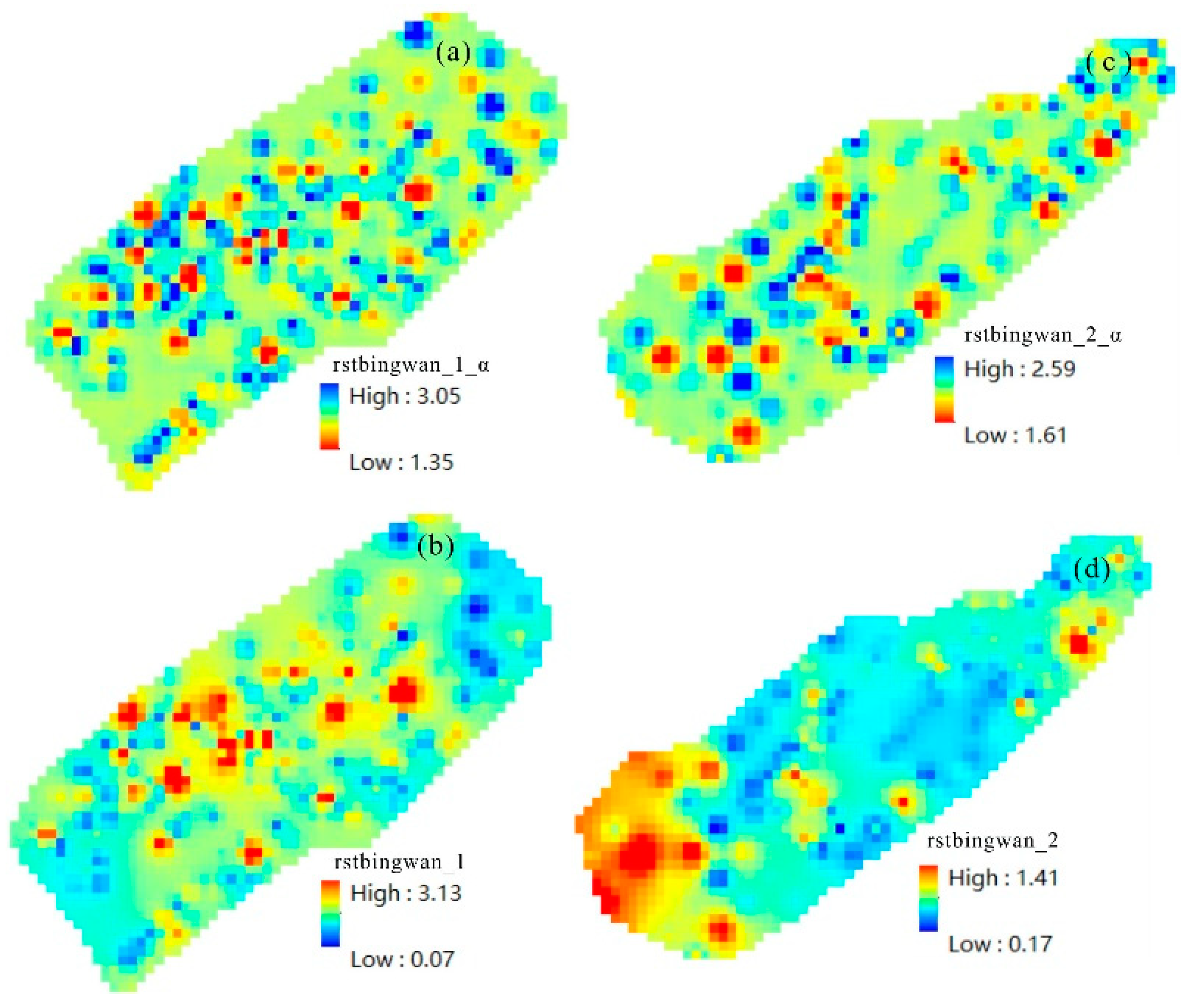
The above-defined anomaly filter and background filter can decompose the original geochemical map into a background map (Figure 7a,c) and anomaly map (Figure 7b,d). In the background map, the trend of the Jiulongjiang Depression and Jinjiang Depression is shown, with the west high and east low pattern. In the anomaly map, the local anomalies of the Jiulongjiang Depression and Jinjiang Depression are more clearly displayed compared to Figure 6, as it removes the interference from the background.

4.3. Integrated Model (CLA-PCA-LSP)

The analysis of singularity conducted earlier takes into account the influence of all indicators in the study area. However, not all indicators need to be included in the calculation to obtain satisfactory results. We can use methods such as cluster analysis to identify the oil and gas indicators that are favorable for hydrocarbon accumulation in the area.

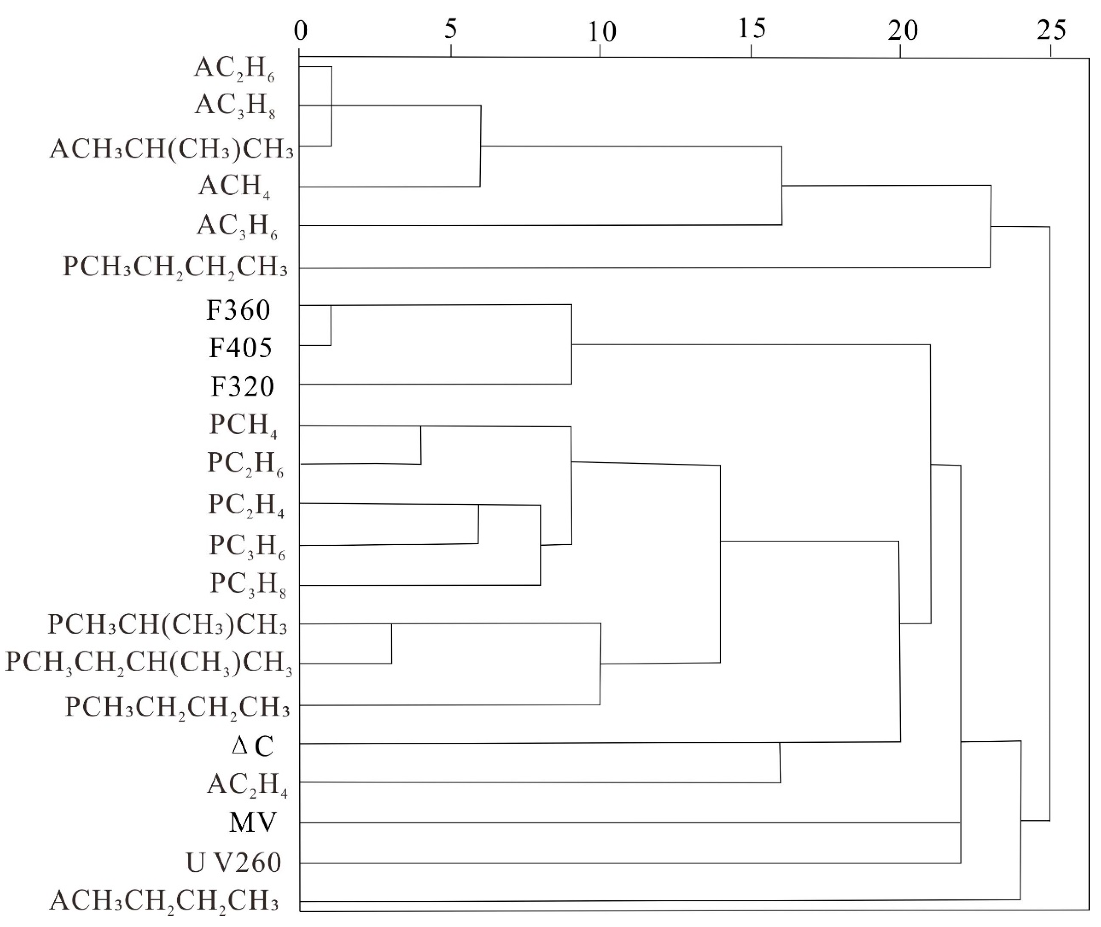
In this study, a cluster analysis was performed on all oil and gas indicators in the Taiwan Strait Basin. The results of the cluster analysis are shown in Figure 8. The analysis divided the indicators into two groups. The first group includes acid-extractable hydrocarbons ethane, propane, isobutane, methane, propylene, and thermally released n-pentane. The second group includes total polycyclic aromatic hydrocarbons at 320 nm, 360 nm, and 405 nm, as well as thermally released methane, ethane, ethylene, propylene, propane, isobutane, isopentane, n-butane, ΔC, MV, acid-extractable ethylene, and total aromatic hydrocarbons and derivatives at 260 nm.

Subsequently, a principal component analysis (PCA) was performed on the results of the cluster analysis for each group (Figure 9). The analysis revealed that the abnormal results identified by the indicators in the second group were similar to the abnormal results identified when considering all indicators (Figure 6). This indicates that the second group of indicators extracted using cluster analysis can effectively indicate the abnormality in the area.

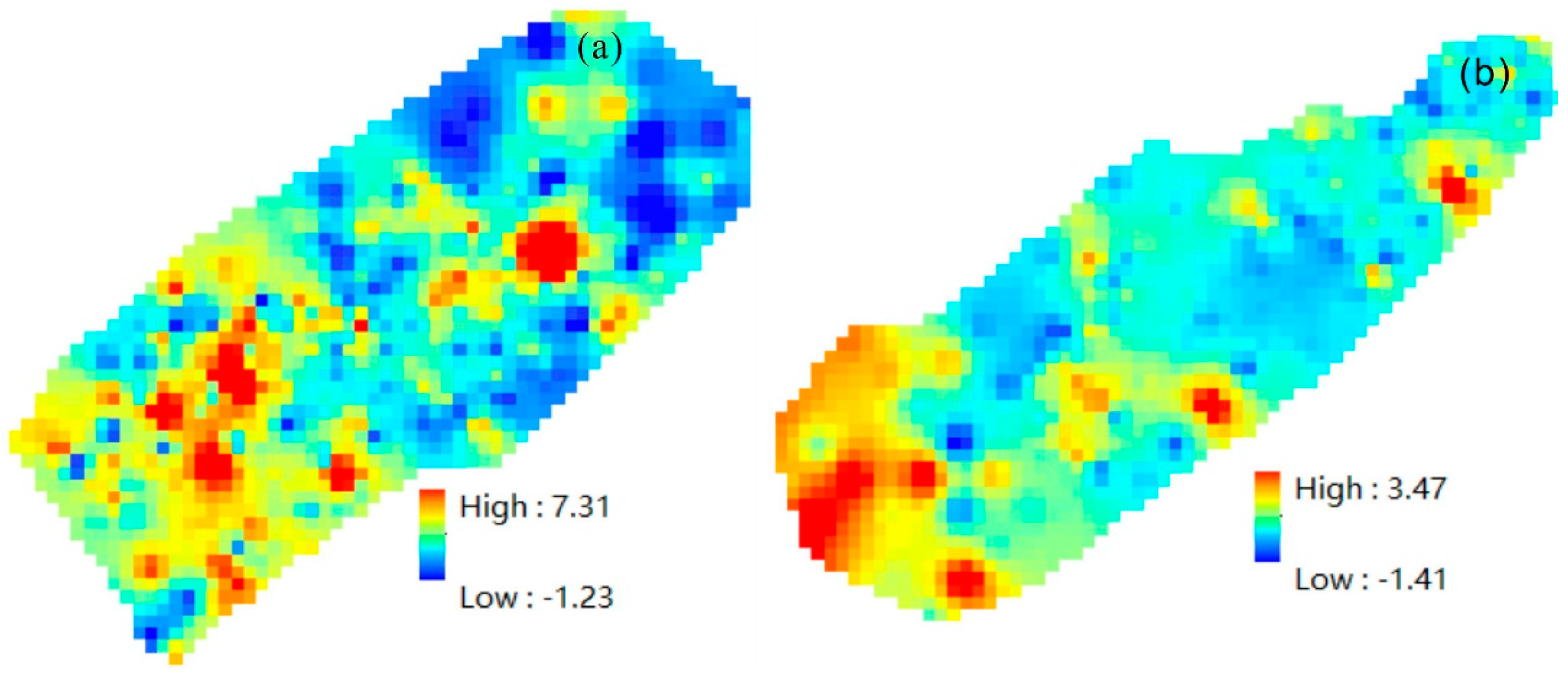
The PCA was performed on the indicators extracted by cluster analysis (Figure 9), and then their singularity indices were calculated. The results are shown in Figure 10. From Figure 10, it can be observed that the singularity indices calculated after the PCA of the selected indicators are very similar to those obtained by the PCA using the complete set of indicators, which further demonstrates that, for the research areas of Jiulongjiang Depression and Jinjiang Depression, we can select favorable oil and gas indicators for analysis instead of including all indicators in the analysis scope, thus improving the efficiency of our calculations.

The results in Figure 4 were obtained by first calculating the local singularity index for each indicator, and then performing a principal component analysis on the obtained multi-indicator singularity index to obtain the score of the first principal component. On the other hand, the results in Figure 10 were obtained by first performing a cluster analysis on the multi-indicators to extract a subset of indicators for the principal component analysis, obtaining the first principal component and then calculating the local singularity index for anomalies. After comparing the results presented in Figure 4 and Figure 10, it is evident that these two methodologies yield highly comparable outcomes, indicating the insensitivity of the singularity index towards regional background field reflections. It is pertinent to compare the outcomes of the CLA-PCA-LSP hybrid model with those derived from PCA-LSP. As illustrated in the ratio result graph (Figure 11) provided below, the range of the ratio results is approximately 1, which quantitatively indicates that the results from these two models are closely aligned, thereby supporting this conclusion. The delineated anomalous results can inform future exploration efforts in the Taiwan Strait Basin. The subsequent identification of favorable exploration areas based on seismic data further substantiates the reliability of our research findings. By integrating these results with the geophysical data from the study area, we delineated comprehensive anomaly information for the Jinjiang Depression and Jiulongjiang Depression, thereby refining our exploration targets and enhancing exploration efficiency.

5. Conclusions

This study investigates the application of nonlinear theory and methods, and unsupervised machine learning algorithms for data processing and anomaly delineation of geochemical indicators in the Taiwan Strait Basin. Local singularity principle (LSP), combined with principal component analysis (PCA) and clustering analysis, was used to comprehensively analyze the geochemical indicators and identify anomalies. The following conclusions are drawn:

The local singularity principle and the generalized self-similarity principle were applied to extract geochemical information of oil and gas indicators in the Taiwan Strait Basin, highlighting key techniques such as identifying weak anomalies, decomposing complex anomalies, and integrating spatial information. The combination of local singularity principle and the S-A method delineates composite anomalies that not only reflect the spatial relationship with known oil and gas reservoir distributions but also reveal multiple composite anomalies in unknown areas. Although these anomalies exhibit different characteristics and diversities in terms of intensity and size, they exhibit self-similarity in the frequency domain.

The use of unsupervised machine learning algorithms for extracting all oil and gas indicators improves model performance and reduces the complexity of multiple calculations. For the Jiulongjiang Depression and Jinjiang Depression study areas, a clustering analysis was applied to extract indicators, followed by a principal component analysis and the calculation of their singularity index to select favorable oil and gas indicators for exploration analysis, thereby improving the efficiency of anomaly delineation calculations.

References

1. Agterberg, F.P.; Bonham-Carter, G.F.; Wright, D.F. Statistical pattern integration for mineral exploration. In Computer Applications in Resource Estimation; Gaál, G., Merriam, D.F., Eds.; Pergamon Press: Oxford, UK, 1990. [Google Scholar] [CrossRef]
2. Herrington, R. Mining our green future. Nat. Rev. Mater. 2021, 6, 456–458. [Google Scholar] [CrossRef]
3. Calvo, G.; Valero, A. Strategic mineral resources: Availability and future estimations for the renewable energy sector. Environ. Dev. 2022, 41, 100640. [Google Scholar] [CrossRef]
4. Carranza, E.J.M.; Mangaoang, J.C.; Hale, M. Application of mineral exploration models and GIS to generate mineral potential maps as input for optimum land-use planning in the Philippines. Nat. Resour. Res. 1999, 8, 165–173. [Google Scholar] [CrossRef]
5. Aranha, M.; Porwal, A.; González-Álvarez, I. Targeting REE deposits associated with carbonatite and alkaline complexes in Northeast India. Ore Geol. Rev. 2022, 148, 105026. [Google Scholar] [CrossRef]
6. Carranza, E.J.M.; Sadeghi, M. Predictive mapping of prospectivity and quantitative estimation of undiscovered VMS deposits in Skellefte district (Sweden). Ore Geol. Rev. 2010, 38, 219–241. [Google Scholar] [CrossRef]
7. Carranza, E.J.M. Geocomputation of mineral exploration targets. Comput. Geosci. 2011, 37, 1907–1916. [Google Scholar] [CrossRef]
8. Chudasama, B.; Porwal, A.; González-Álvarez, I.; Thakur, S.; Wilde, A.; Kreuzer, O.P. Calcrete-hosted surficial uranium systems in Western Australia: Prospectivity modeling and quantitative estimates of resources. Part 1—Origin of calcrete uranium deposits in surficial environments: A review. Ore Geol. Rev. 2018, 102, 906–936. [Google Scholar] [CrossRef]
9. Esmaeiloghli, S.; Tabatabaei, S.H.; Carranza, E.J.M. Spatio-Geologically Informed Fuzzy Classification: An innovative Method for Recognition of MineralizationRelated patterns by Integration of Elemental, 3D Spatial, and Geological Information. Nat. Resour. Res. 2021, 30, 989–1010. [Google Scholar] [CrossRef]
10. Cheng, Q.M.; Agterberg, F.P.; Ballantyne, S.B. The separation of geochemical anomalies from background by fractal methods. J. Geochem. Explor. 1994, 51, 109–130. [Google Scholar] [CrossRef]
11. Govett, G.; Goodfellow, W.; Chapman, R.; Chork, C. Exploration geochemistry—Distribution of elements and recognition of anomalies. J. Int. Assoc. Math. Geol. 1975, 7, 415–446. [Google Scholar] [CrossRef]
12. El-Makky, A.M. Statistical analyses of La, Ce, Nd, Y, Nb, Ti, P, and Zr in bedrocks and their significance in geochemical exploration at the Um Garayat Gold mine area, Eastern Desert, Egypt. Nat. Resour. Res. 2011, 20, 157. [Google Scholar] [CrossRef]
13. Chiles, J.-P.; Delfiner, P. Geostatistics: Modeling spatial uncertainty. In Probability and Statistics; Wiley Series: Hoboken, NJ, USA, 2012. [Google Scholar]
14. Wang, H.; Zuo, R. A comparative study of trend surface analysis and spectrumarea multifractal model to identify geochemical anomalies. J. Geochem. Explor. 2015, 155, 84–90. [Google Scholar] [CrossRef]
15. Bigdeli, A.; Maghsoudi, A.; Ghezelbash, R. Recognizing geochemical anomalies associated with mineral resources using singularity analysis and random forest models in the Torud-Chahshirin Belt, Northeast Iran. Minerals 2023, 13, 1399. [Google Scholar] [CrossRef]
16. Ghezelbash, R.; Maghsoudi, A.; Carranza, E.J.M. Optimization of geochemical anomaly detection using a novel genetic K-means clustering (GKMC) algorithm. Comput. Geosci. 2020, 134, 104355. [Google Scholar] [CrossRef]
17. Chen, Y.; Zhao, Q.; Lu, L. Combining the outputs of various k-nearest neighbor anomaly detectors to form a robust ensemble model for high-dimensional geochemical anomaly detection. J. Geochem. Explor. 2021, 231, 106875. [Google Scholar] [CrossRef]
18. Bigdeli, A.; Maghsoudi, A.; Ghezelbash, R. Application of self-organizing map (SOM) and K-means clustering algorithms for portraying geochemical anomaly patterns in Moalleman district, NE Iran. J. Geochem. Explor. 2022, 233, 106923. [Google Scholar] [CrossRef]
19. Zhang, L.; Xu, G.Q.; Lin, Z. Stratigraphic and Sedimentary Evolution of the Northern Continental Slope of the South China Sea and the Taiwan Strait; Geological Publishing House: Beijing, China, 2019; Volume 12, pp. 137–139. [Google Scholar]
20. Zhang, Y.; Zhang, L.; Xiao, F.; Zhao, J.; Lei, Z.; Qian, X. Fractal modeling of oil and gas geochemical data in the Taiwan Strait Basin. J. Geochem. Explor. 2023, 257, 107353. [Google Scholar] [CrossRef]
21. Cheng, Q.M. Singularity theory and methods for mapping geochemical anomalies caused by buried sources and for predicting undiscovered mineral deposits in covered areas. J. Geochem. Explor. 2012, 122, 55–70. [Google Scholar] [CrossRef]
22. Cheng, Q.M.; Xu, Y.G.; Grunsky, E. Integrated spatial and spectrum method for geochemical anomaly separation. Nat. Resour. Res. 2000, 9, 43–51. [Google Scholar] [CrossRef]
23. Cheng, Q.M. Multifractality and spatial statistics. Comput. Geosci. 1999, 25, 949–961. [Google Scholar] [CrossRef]
24. Reimann, C.; de Caritat, P. Establishing geochemical background variation and threshold values for 59 elements in Australian surface soil. Sci. Total Environ. 2017, 578, 633–648. [Google Scholar] [CrossRef] [PubMed]
25. Ghezelbash, R.; Maghsoudi, A.; Bigdeli, A.; Carranza, E.J.M. Regional-scale mineral prospectivity mapping: Support vector machines and an improved data-driven multi-criteria decision-making technique. Nat. Resour. Res. 2021, 30, 1977–2005. [Google Scholar] [CrossRef]
26. Templ, M.; Filzmoser, P.; Reimann, C. Cluster analysis applied to regional geochemical data: Problems and possibilities. Appl. Geochem. 2008, 23, 2198–2213. [Google Scholar] [CrossRef]
27. Meng, H.D.; Song, Y.C.; Song, F.Y.; Shen, H.T. Research and application of cluster and association analysis in geochemical data processing. Comput. Geosci. 2011, 15, 87–98. [Google Scholar] [CrossRef]
28. Morrison, J.M.; Goldhaber, M.B.; Ellefsen, K.J.; Mills, C.T. Cluster analysis of a regional-scale soil geochemical dataset in northern California. Appl. Geochem. 2011, 26, S105–S107. [Google Scholar] [CrossRef]
29. Yu, X.T.; Xiao, F.; Zhou, Y.Z.; Wang, Y.; Wang, K.Q. Application of hierarchical clustering, singularity mapping, and Kohonen neural network to identify Ag-Au-Pb Zn polymetallic mineralization associated geochemical anomaly in Pangxidong district. J. Geochem. Explor. 2019, 203, 87–95. [Google Scholar] [CrossRef]
Figure 1. Regional geological background map and scope of study area.
Fractalfract 08 00553 g001
Figure 2. (a) The singularity index of thermal hydrocarbon propane in the Jiulongjiang Depression, and (b) the original data plot of thermal hydrocarbon propane in the Jiulongjiang Depression. On the other hand, (c) the singularity index of thermal hydrocarbon propane in the Jinjiang Depression, and (d) 4the original data plot of thermal hydrocarbon propane in the Jinjiang Depression.
Fractalfract 08 00553 g002
Figure 3. (a) The singularity index of total polycyclic aromatic hydrocarbons at 405 nm in the Jiulongjiang Depression, and (b) the original data plot of total polycyclic aromatic hydrocarbons at 405 nm in the Jiulongjiang Depression. Similarly, (c) the singularity index of total polycyclic aromatic hydrocarbons at 405 nm in the Jinjiang Depression, and (d) the original data plot of total polycyclic aromatic hydrocarbons at 405 nm in the Jinjiang Depression.
Fractalfract 08 00553 g003
Figure 4. The results of principal component analysis on all indicator singular values (α values) are presented in (a) (for the Jiulongjiang Depression) and (b) (for the Jinjiang Depression).
Fractalfract 08 00553 g004
Figure 5. PCA results of the logarithmically transformed values of all indicators, including the distribution of eigenvalues (a) and the loading plot of the first principal component (b), which represents the contribution of each indicator to the first principal component (Taking Jiulongjiang Depression as an example).
Fractalfract 08 00553 g005
Figure 6. (a) The first principal component loadings map (Jiulongjiang Depression) obtained by logarithmic transformation of all indicators. (b) The S-A curve of loadings in the first principal component (Jiulongjiang Depression). (c) The first principal component load diagram obtained after the logarithmic transformation of all indexes (Jinjiang Depression), (d) The S-A curve of the load in the first principal component (Jinjiang Depression).
Fractalfract 08 00553 g006
Figure 7. (a) The decomposed background field of the first principal component load of the Jiulongjiang Depression, (b) the decomposed anomaly field of the first principal component load of the Jiulongjiang Depression, (c) the decomposed background field of the first principal component load of the Jinjiang Depression, (d) the decomposed anomaly field of the first principal component load of the Jinjiang Depression.
Fractalfract 08 00553 g007
Figure 8. Cluster analysis results of all indicators.
Fractalfract 08 00553 g008
Figure 9. The first principal component loadings obtained from PCA of the indicators extracted by cluster analysis for the Jiulongjiang Depression (a) and Jinjiang Depression (b).
Fractalfract 08 00553 g009
Figure 10. The singularity index calculated after performing PCA on the selected indicators from cluster analysis for the Jiulongjiang Depression (a) and Jinjiang Depression (b).
Fractalfract 08 00553 g010
Figure 11. The ratio result between Figure 4 and Figure 10 for the Jiulongjiang Depression (a) and Jinjiang Depression (b).
Fractalfract 08 00553 g011