A Novel Fractional Model and Its Application in Network Security Situation Assessment

Abstract

The evaluation process of the Fractional Order Model is as follows. To address the commonly observed issue of low accuracy in traditional situational assessment methods, a novel evaluation algorithm model, the fractional-order BP neural network optimized by the chaotic sparrow search algorithm (TESA-FBP), is proposed. The fractional-order BP neural network, by incorporating fractional calculus, demonstrates enhanced dynamic response characteristics and historical dependency, showing exceptional potential for handling complex nonlinear problems, particularly in the field of network security situational awareness. However, the performance of this network is highly dependent on the precise selection of network parameters, including the fractional order and initial values of the weights. Traditional optimization methods often suffer from slow convergence, a tendency to be trapped in local optima, and insufficient optimization accuracy, which significantly limits the practical effectiveness of the fractional-order BP neural network. By introducing cubic chaotic mapping to generate an initial population with high randomness and global coverage capability, the exploration ability of the sparrow search algorithm in the search space is effectively enhanced, reducing the risk of falling into local optima. Additionally, the Estimation of Distribution Algorithm (EDA) constructs a probabilistic model to guide the population toward the globally optimal region, further improving the efficiency and accuracy of the search process. The organic combination of these three approaches not only leverages their respective strengths, but also significantly improves the training performance of the fractional-order BP neural network in complex environments, enhancing its generalization ability and stability. Ultimately, in the network security situational awareness system, this integration markedly enhances the prediction accuracy and response speed.

1. Introduction

In the complex environment of naval battlefield electronic information systems, network security situational prediction faces multiple challenges, including high precision, real-time performance, and robustness. To address these issues, this paper proposes a network security situational assessment model based on the TESA-FBP (fractional-order BP neural network optimized by the chaotic sparrow search algorithm) to enhance the performance of network security situational prediction models. Although traditional BP neural networks possess strong nonlinear mapping capabilities [1,2,3], they often exhibit slow convergence and a tendency to become trapped in local optima when dealing with highly dynamic and limited data scenarios typical of network security situational predictions, rendering them inadequate for the stringent demands of naval battlefield electronic information systems.

By leveraging the long memory characteristics of fractional calculus [4,5,6,7,8], the BP neural network’s ability to respond to complex situational changes is enhanced, thereby addressing the limitations of traditional integer-order models in handling multiscale problems. Furthermore, to mitigate the impact of initial weight settings on model prediction accuracy, this paper proposes using cubic chaotic mapping to generate an initial population with high randomness and coverage, thereby improving the global exploration capability of the sparrow search algorithm and reducing the risk of the network becoming trapped in local optima during the early stages of training. Building on this, to further enhance the accuracy and efficiency of network weight optimization, the paper integrates the Estimation of Distribution Algorithm (EDA), which constructs a probabilistic model to guide the population toward the globally optimal solution. This approach effectively avoids the local convergence issues common in traditional optimization algorithms when dealing with complex multimodal problems, significantly improving the accuracy and stability of network security situational predictions.

2. Materials and Methods

2.1. Fundamental Theory of Fractional Calculus

Fractional calculus, an important branch of calculus, dates back to the 17th century and has evolved alongside integer-order calculus. Scholars such as L’Hospital were pioneers in proposing the concept of fractional calculus, which has since generated considerable academic interest. Fractional calculus extends integer-order calculus by allowing differentiation and integration orders to be real numbers. When the order is an integer, fractional calculus is reduced to integer-order calculus; when the order is fractional, its unique properties become apparent. However, due to the theoretical and modeling complexities and early computational limitations, solving problems in fractional calculus was once challenging, making its practical application in engineering difficult and limiting its early adoption.

In the 21st century, the rapid advancement of computer technology has renewed interest in fractional calculus. These technological breakthroughs have simplified the solving process and significantly reduced computational demands. Scholars have discovered that many natural phenomena are difficult to describe accurately using traditional integer-order models, while fractional calculus offers greater flexibility and precision. As a result, fractional calculus has been widely applied in fields such as control systems [9,10], image processing [11,12,13], and chaotic dynamics [14,15], achieving significant results. Today, fractional calculus has become a research hotspot, and its potential applications are continually being explored. With ongoing research and technological progress, fractional calculus is expected to play a more significant role in advancing various disciplines.

The theoretical framework of fractional calculus has now matured with extensive applications in both theoretical research and engineering practice. Its definitions are diverse, including those of Caputo, Grunwald-Letnikov, Cauchy, and Riemann-Liouville, each possessing unique features and interconvertibility. The Caputo definition is particularly noted for its simplicity and practicality.

Traditional gray models are constrained by first-order fitting equations; however, the introduction of fractional-order theory has effectively broadened their application scope. This combination retains the simplicity of the gray models while significantly enhancing their predictive performance. Therefore, integrating fractional calculus with gray models represents a practical and effective improvement with important implications for research and applications across multiple fields.

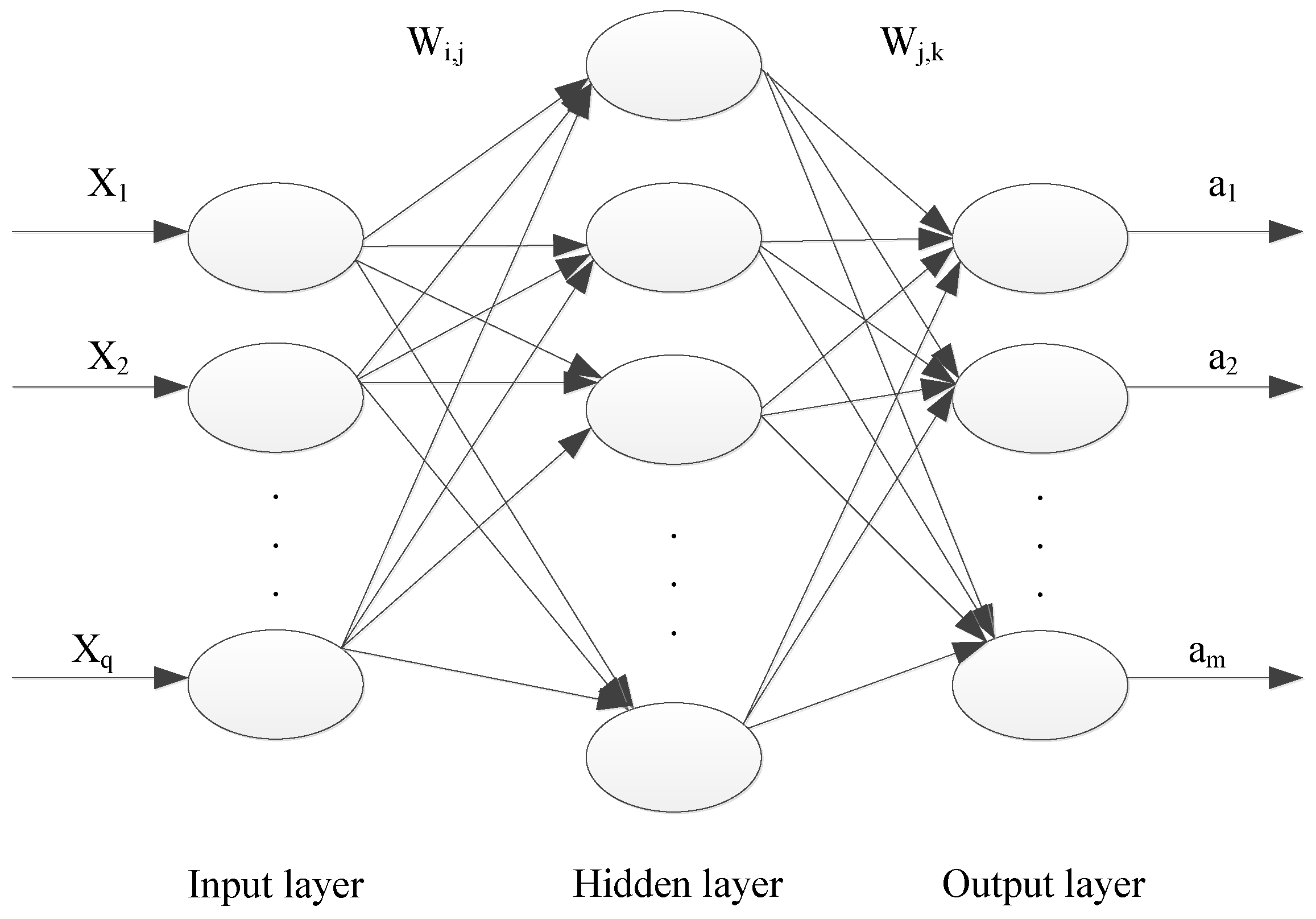
2.2. Fundamental Theory of BP Neural Networks

BP neural networks are multilayer feedforward networks based on the error backpropagation algorithm. These networks simplify biological models [16,17] and are currently among the most widely used and popular neural network models [18]. Typically, by employing the gradient descent algorithm, BP neural networks can perform various nonlinear mappings, including input-to-output mappings. The BP algorithm is known as the backpropagation learning algorithm [19] because the network weights are adjusted based on the difference between the actual and desired outputs, with the adjustment process occurring in a backward manner. BP networks are primarily used for function approximation and pattern recognition, achieving widespread applications [20,21,22,23,24,25,26,27,28].

2.3. Basic Principles of BP Neural Networks

BP neural networks (BPNN, BP) are common neural network models. Their primary structure, as illustrated in Figure 1, comprises an input layer, multiple hidden layers, and an output layer. The nodes in each layer are interconnected through connection weights without interfering with each other.

Figure 1. The model of a BP neural network.

2.4. Fractional BP Neural Network

2.4.1. Caputo Fractional Derivative

For a function $f\left(t\right)$, its first-order causal derivative can be written as

$$D_{l}f\left(t\right)={lim}_{h\to 0^{+}} {\displaystyle \frac{f\left(t\right)-f(t-h)}{h}}$$

(1)

Combining this with the Caputo fractional calculus formula yields the definition of the Caputo fractional causal derivative.

$${}_{t_0}{}^{C}D_t^{\alpha }f(t)={\displaystyle \frac{1}{\Gamma (m-\alpha )}}{\int }_{t_0}^t {\displaystyle \frac{f^{\left(m\right)}(\tau )}{(t-\tau {)}^{\alpha -m+1}}}d\tau$$

(2)

where ${}_{a}D_t^{\alpha }$ denotes the Caputo fractional operator, $\alpha$ is the fractional order, and $\left[a,t\right]$ is the integration interval of $f\left(t\right)$. When $\alpha$ is in the interval (0, 1), the formula becomes

$${}_{l}Caputo {}_{a}D_t^{\alpha }f(t)={\displaystyle \frac{1}{\Gamma (1-\alpha )}}{\int }_a^t (t-\tau {)}^{-\alpha }\cdot f^{\prime }(\tau )d\tau$$

(3)

The Caputo fractional derivative offers the following several key advantages

Physical Interpretability: The Caputo fractional derivative retains some of the physical interpretability of classical integer-order calculus, particularly in the setting of the initial conditions. It allows for the use of traditional initial condition forms within fractional-order models, ensuring that the training and optimization process of the network remains consistent with the physical context of the application.

Ease of Handling Initial Conditions: Within the framework of the Caputo fractional derivative, the initial conditions can be maintained in the same form as those in traditional integer-order derivatives. This is particularly important in fractional-order BP neural networks for handling boundary and initial value problems, as it avoids the complexity of calculating the initial conditions associated with other types of fractional derivatives.

Smooth Memory Effect: The Caputo fractional derivative better captures the memory characteristics and historical dependencies of the system, which is especially effective for BP neural networks dealing with time-series data or data with long-term dependencies. The Caputo derivative introduces a smooth memory effect, enabling the network to more accurately reflect the influence of past inputs during optimization, thereby improving the predictive performance.

Relative Computational Simplicity: Compared to other forms of fractional derivatives, such as the Riemann-Liouville derivative, the Caputo fractional derivative is relatively simpler to implement numerically. This simplicity reduces the computational burden during the training of complex BP neural networks, thereby facilitating more efficient training and optimization.

Overall, the application of the Caputo fractional derivative in fractional-order BP neural networks balances physical interpretability, computational simplicity, and the capture of system memory effects, making it a preferred choice for optimizing network performance.

2.4.2. Caputo Fractional BP Neural Network

Let the number of neurons in the input layer, hidden layer, and output layer of a BP neural network be m, n, and l, respectively, with a sample size of J. The input sample j (j $\in$ J) and its expected output are denoted as $X^j$ and $O^j$. Let $W1={\left({\nu }_{iq}\right)}_{n\times m}$ represent the weights between the input and hidden layers, and $W2={\left({\mu }_1,{\mu }_2,\cdots ,{\mu }_n\right)}^T$ represent the weights between the hidden and output layers, where i, q are the weights corresponding to neurons in the input and hidden layers, and ${\mathsf{\mu }}_{\mathrm{p}}$ are the weights corresponding to neurons in the p hidden layer and the output layer. Assume that the transfer function of the hidden layer is $\mathrm{g}$, and the transfer function of the output layer is $f$.

Define ${\theta }^{i,j}={\nu }_{i1}{x}_1^j+{\nu }_{i2}{x}_2^j+\cdots +{\nu }_{im}{x}_m^j={\nu }_i\cdot X^j$ representing the input from sample j to the hidden layer neuron i. The input to the output layer is ${\xi }^j=W2\cdot G\left(W1\cdot X^j\right)$, and the actual output is $y^j=f\left(W_2\cdot G\left(W1X^j\right)\right.$. The error function of the weights can be expressed as

$$E\left(W\right)={\displaystyle \frac{1}{2}}{\sum }_{j=1}^J {\left(O^j-f\left(W2\cdot G\left(W1\cdot X^j\right)\right)\right)}^2={\sum }_{j=1}^J f_j\left(W2\cdot G\left(W1\cdot X^j\right)\right)$$

(4)

Here, $f_j(t)={\displaystyle \frac{1}{2}}{\left(O^j-f(t)\right)}^2, t\in R, f_j(\cdot )$ is composed of functions $G$ and $f$; initial weights are $W^0=\left(W{1}^0,W{2}^0\right)$; and weights at iteration $W^k=\left(W{1}^k,W{2}^k\right)$.

The error function’s partial derivative with respect to the weights using Caputo fractional calculus can be expressed as

$$\begin{array}{rr}{\mu }_i^{k+1}& ={\mu }_i^k-\eta \cdot {}_{l}Caputo_{cmin}{D}_{{\mu }_i^k}^{\alpha }E(W)\\ {\nu }_{ir}^{k+1}& ={\nu }_{ir}^k-\eta \cdot {}_{l}Caputo_{cmin}{D}_{{\nu }_{ir}^k}^{\alpha }E(W)\end{array}$$

(5)

where $\eta >0$ is the learning rate; $\alpha$ is the fractional order; and $h\left(s\right(t\left)\right)$ is a composite function. According to the definition of the Caputo fractional derivative, $h\left(s\right(t\left)\right)$ with respect to $t$ of order $\alpha$ is

From Equation (5), we can obtain ${}_{l}Caputo_{cmin}{D}_{{\nu }_{ir}^k}^{\alpha }E\left(W\right)\mathrm{a}\mathrm{n}\mathrm{d}{}_{l}Caputo_{cmin}{D}_{{\nu }_{ir}^k}^{\alpha }E(W)$.

First, for

$${}_{l}Caputo_{cmin}{D}_{{\mu }_i^k}^{\alpha }E\left(W\right):{}_{l}Caputo_{cmin}{D}_{{\nu }_{ir}^k}^{\alpha }E\left(W\right)={\displaystyle \frac{\partial E\left(W\right)}{\partial {\zeta }^j}}\cdot {}_{l}Caputo_{cmin}{D}_{{\mu }_i^k}^{\alpha }\left({\zeta }^j\right)$$

(6)

where ${\displaystyle \frac{\partial E\left(W\right)}{\partial {\zeta }^j}}={\sum }_{j=1}^J f_j^{\prime }\left(W2\cdot G\left(W1\cdot X^j\right)\right)$. When $0<\alpha <1$, it can be expressed as

$$\begin{array}{c}{}_{l}Caputo_{cmin}{D}_{{\mu }_i^k}^{\alpha }\left({\zeta }^j\right)={\displaystyle \frac{1}{\Gamma \left(1-\alpha \right)}}{\int }_{cmin}^{{\mu }_i^k} {\left({\mu }_i^k-\tau \right)}^{-\alpha }·g\left({\nu }_i^k\cdot X^j\right)d\tau ={\displaystyle \frac{1}{\Gamma (1-\alpha )}}g\left({\nu }_i^k\cdot X^j\right){\int }_{cmin}^{{\mu }_i^k} {\left({\mu }_i^k-\tau \right)}^{-\alpha }d\tau \\ \\ ={\displaystyle \frac{1}{\Gamma (1-\alpha )}}{\displaystyle \frac{1}{1-\alpha }}g\left({\nu }_i^k\cdot X^j\right){\left({\mu }_i^k-cmin\right)}^{1-\alpha }\end{array}$$

(7)

Therefore, the specific formula for the error with respect to ${\mu }_i^k$ is

$$\begin{array}{c}{}_{l}Caputo_{cmin}{D}_{{\mu }_i^k}^{\alpha }E(W)={\displaystyle \frac{1}{(1-\alpha )\Gamma (1-\alpha )}}\cdot {\sum }_{j=1}^J f_j^{\prime }(W2\cdot \\ \left.G\left(W1\cdot X^j\right)\right)g\left({\nu }_i^k\cdot X^j\right){\left({\mu }_i^k-cmin\right)}^{1-\alpha }\end{array}$$

(8)

Next, for ${}_{l}Caputo_{cmin}{D}_{{\nu }_{ir}^k}^{\alpha }E(W)$, similarly:

$${}_{l}Caputo_{cmin}{D}_{{\nu }_{ir}^k}^{\alpha }E(W)={\displaystyle \frac{\partial E\left(W\right)}{\partial {\theta }^{i,j}}}\cdot {}_{l}Caputo_{cmin}{D}_{{\nu }_{ir}^k}^{\alpha }\left({\theta }^{i,j}\right)\mathrm{where}{\displaystyle \frac{\partial E\left(W\right)}{\partial {\theta }^{i,j}}}={\sum }_{j=1}^J f_j^{\prime }\left(W2\cdot G\left(W1X^j\right)\right){\mu }_i{g}^{\prime }\left({\nu }_i\cdot X^j\right).$$

The Caputo fractional derivative of ${\theta }^{i,j}$ with respect to ${\nu }_{ir}^k$ is

$$\begin{array}{c}{}_{l}Caputo_{cmin}{D}_{{\nu }_{ir}^k}^{\alpha }\left({\theta }^{i,j}\right)={\displaystyle \frac{1}{\Gamma (1-\alpha )}}{\int }_{cmin}^{{\nu }_{ir}^k} {\left({\nu }_{ir}^k-\tau \right)}^{-\alpha }{x}_r^{j}d\tau =\\ {\left.{\displaystyle \frac{1}{\Gamma (1-\alpha )}}{x}_r^j{\displaystyle \frac{1}{1-\alpha }}{\left({\nu }_{ir}^k-\tau \right)}^{-\alpha }\right|}_{cmin}^{{\nu }_{ir}^k}=\\ {\displaystyle \frac{1}{(1-\alpha )\Gamma (1-\alpha )}}{x}_r^j{\left({\nu }_{ir}^k-c_{min}\right)}^{1-\alpha }\end{array}$$

(9)

${\nu }_{ir}^k$: Represents the input value for the rrr-th neuron in the kkk-th layer for the iii-th sample. It typically indicates the input signal at a particular layer of a neural network.

${\theta }^{i,j}$: Denotes the weight parameter between the jjj-th neuron and a target neuron for the iii-th sample. This parameter is generally the weight that is optimized during the training of the neural network.

$\alpha$: The fractional order of the derivative, ranging between 0 and 1, representing the fractional order of the derivative.

$c\min$ representing the fractional order of the derivative between 0 and 1 target neuron for the iii-th sample. This parameter is generally the weight that is optimized during the training of the neural network

$\Gamma (1-\alpha )$: The Gamma function, used to calculate the normalization constant in the fractional derivative. The Gamma function is a common special function in fractional calculus.

$x_r^j$: Represents the value of the jjj-th input signal received by the rrr-th neuron. It usually indicates either the input signal from the input layer or the output signal from the previous layer.

$r$: The integration variable, representing a variable over time or space, used to define the integration range from $c\min$ to ${\nu }_{ir}^k$.

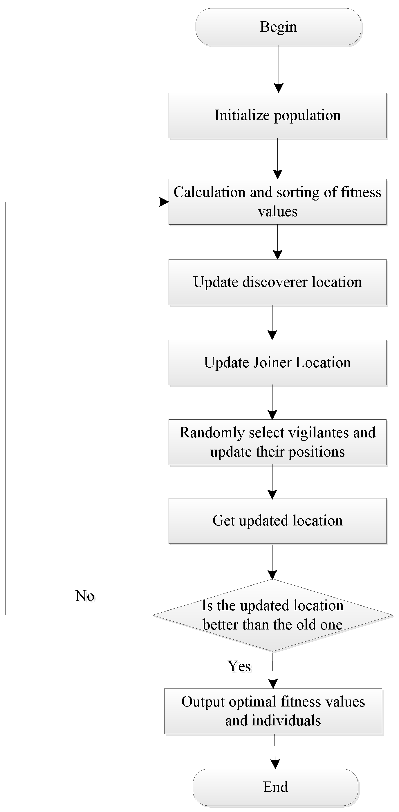
2.5. Fundamental Theory of the Sparrow Search Algorithm

2.5.1. Mathematical Model of the Algorithm

In 2020, Xue Jiankai proposed a novel swarm intelligence algorithm known as the sparrow search algorithm (SSA). Compared to other swarm intelligence optimization algorithms, SSA demonstrates exceptional performance in terms of search accuracy, faster convergence speed, and relatively stable performance, and has gradually attracted the attention of many scholars. The inspiration for this algorithm comes from the foraging and anti-predation behavior of sparrows in nature.

In SSA, there are three roles: discoverers, joiners, and scouts. Discoverers are responsible for finding food and guiding the direction of the entire population. Joiners search for food based on the information provided by discoverers, often acting together to find food sources. Scouts monitor and compete with discoverers for food and stop foraging when the entire population faces predation threats or perceives danger.

The mathematical model for the discoverers is shown in Equation (10):

$$X_{i,d}^{t+1}=\left\{\begin{array}{c}{X}_{i,d}^t\cdot exp\left({\displaystyle \frac{-i}{\alpha \cdot G}}\right) if R_2<ST\\ X_{i,d}^t+Q\cdot L if R_2\ge ST\end{array}\right.$$

(10)

In the formula, $t$ represents the current iteration number, $G$ is the maximum number of iterations, $X_{i,d}$ is the position information of the $\mathrm{i}$-th sparrow, $\alpha \in (0,1]$ is a random number, $ST$ is the safety value, $R_2$ is a random number in the interval (0, 1), $Q$ is a normally distributed random number, and $L$ is a 1 × d matrix. The mathematical model for the joiners is shown in Equation (11):

$$X_{i,d}^{t+1}=\left\{\begin{array}{c}Q\cdot exp\left({\displaystyle \frac{X_{worst}^t-X_{i,d}^t}{i^2}}\right) if i>n/2\\ X_P^{t+1}+\left|X_{i,d}^t-X_P^{t+1}\right|\cdot A^{+}\cdot L otherwise\end{array}\right.$$

(11)

In the formula, $X_P$ denotes the position of the discoverer; $X_{worst}^t$ is the worst position in the population; $Q$ is a random number following a standard Gaussian distribution; and $A$ is a $1\times d$ matrix, with $A^{+}=A^T{\left(A{A}^T\right)}^{-1}$. The mathematical model for scouts is described as follows (Equation (12)):

$$X_{i,d}^{t+1}=\left\{\begin{array}{ll}{X}_{best}^t+\beta \cdot \left|X_{i,d}^t-X_{best}^t\right|& if f_i>f_g\\ X_{i,d}^t+K\cdot \left({\displaystyle \frac{\left|X_{i,d}^t-X_{worst}^t\right|}{\left(f_i-f_w\right)+\epsilon }}\right)& if f_i=f_g\end{array}\right.$$

(12)

In the formula: $X_{best}^t$ denotes the global optimal position; $\beta$ is a random variable following a standard Gaussian distribution; $f_i$ represents the fitness value of the current sparrow; $f_g$ is the optimal objective function value; $f_w$ is the worst objective function value; and $\epsilon$ is a small constant. A flowchart of the sparrow search algorithm is illustrated in Figure 2.

Figure 2. The flowchart of sparrow search algorithm.

The pseudocode for the sparrow search algorithm is presented in Table 1.

Table 1. Sparrow search algorithm.

The Framework of Sparrow Search Algorithm
input:
G: Maximum Number Of Iterations;
w: Number of Discoverers in Sparrow Population;
SD: Number of vigilantes in the sparrow population;
R2: warning value;
Establish an objective function $F\left(x\right),$ where $N$ $X=x\left(x_1,x_2,\cdots ,x_d\right),$ are initialized, and relevant parameters are defined;
output: $x_{\mathrm{best}},f_g$;
1: while $t\le G;$
2: Sort the fitness values to find the current best individual and the current worst individual;
${3:R}_2=\mathrm{rand}\left(1\right);$
4: for $i=1:N^{\mathrm{*}}w;$
5: Update the position of individual sparrow discoverers using Equation (10);
6: end for;
7: for $i=\left(N^{\mathrm{*}}w+1\right):N;$
8: Use Equation (11) to update the position of individual sparrow joiners;
9: end for;
10: for $i=1:S{D}^{\mathrm{*}}N;$
11: Use Equation (12) to update the position of individual sparrow watchers;
12: end for;
13: Obtain the latest global optimum;
14: $t=t+1;$
15: end while;
16: return $x_{\mathrm{best}},f_g$.

2.5.2. Analysis of the Advantages and Disadvantages of SSA

The sparrow search algorithm (SSA), as an innovative heuristic method, has garnered significant attention in academia due to its rapid convergence, ease of implementation, and minimal parameter tuning. The algorithm demonstrates exceptional performance in a local search. However, like all algorithms, SSA is not without its limitations. The primary drawbacks of the SSA algorithm include the following:

Premature Convergence: When discoverers in the SSA algorithm identify a local optimum, followers quickly converge around this solution. Due to the algorithm’s lack of an effective mechanism to escape local optima, SSA sometimes exhibits low convergence accuracy. This is a critical area for further research and improvement.

Slow Convergence Speed: At the onset of the SSA, both discoverers and followers are randomly generated, resulting in an uneven distribution. Additionally, the ratio of discoverers to followers is preset and fixed, which makes it difficult to adjust strategies flexibly based on real-time environmental changes during iterations. Particularly in the later stages of the iteration, the lack of population diversity often results in a relatively slow convergence rate. This limitation restricts the effectiveness of the SSA in certain complex scenarios, necessitating further research and optimization.

2.6. Fundamental Theory of Chaos

Chaos, as a distinctive phenomenon within deterministic systems, exhibits both chaotic disorder and inherent order. This complex state is prevalent during numerous natural movements and events. The sensitivity of chaotic systems to initial conditions and their intrinsic randomness form a robust foundation for the application of chaos theory across various scientific disciplines, particularly in fields such as artificial intelligence and cryptography. The integration of chaos theory with intelligent algorithms is especially significant.

2.6.1. Definition of Chaos

Chaos is characterized by finite non-periodic motion, with its dynamics concentrated in specific attractor regions. Despite its finite nature, this motion demonstrates marked instability, distinguishing it from quasi-periodic or stable finite motions. There are several definitions of chaos. The Li-Yorke definition provides a rigorous mathematical perspective but is complex and challenging to comprehend. Conversely, the definition proposed by Devaney in 1989 is more accessible and intuitive, making it easier to understand and more widely accepted.

Li-Yorke Definition of Chaos

The Li-Yorke definition of chaos for a continuous self-map $f\left(x\right)$ on an interval $\mathrm{I}$ is as follows:

(1)

The periodic points of $\mathrm{f}$ have unbounded periods.

(2)

For any $x_1,x_2\in S$ where $x_1\ne x_2$, $\underset{n\to \infty }{lim} sup\left|f^n\left(x_1\right)-f^n\left(x_2\right)\right|>0$

(3)

For any $x_1,x_2\in S$, $\underset{n\to \infty }{lim inf} \left|f^n\left(x_1\right)-f^n\left(x_2\right)\right|=0$

(4)

Where $f^n(\cdot )=f(f\cdots f(\cdot \left)\right)$, and for any $\mathrm{x}\in \mathrm{S}$ and any periodic point $y$ of $f$, $\underset{n\to \infty }{lim} sup\left|f^n\left(x\right)-f^n\left(y\right)\right|>0$ Then $\mathrm{f}$ is said to be chaotic on interval $I$.

Based on the Li-Yorke definition of chaos, a chaotic system should possess three core characteristics:

(1)

The system includes a countable number of stable periodic trajectories that exhibit regular and repetitive patterns.

(2)

It also contains numerous unstable non-periodic trajectories that display irregular and unpredictable behavior.

(3)

Crucially, there is at least one unstable non-periodic trajectory, underscoring the complexity and unpredictability of chaotic motion.

Devaney’s Definition of Chaos

Devaney’s definition of chaos states that a continuous map $f:X\to X$ is chaotic if it satisfies:

(1)

$f$ is topologically transitive.

(2)

The periodic points of $f$ are dense in $X$.

(3)

Sensitivity to initial conditions: there exists $\delta >0$, such that for any $\epsilon >0$ and any $x\in X$, there exists $\mathrm{y}$ in the $\mathsf{\epsilon }$-neighborhood of $\mathrm{x}$ and a natural number $\mathrm{n}$ such that $d\left(f^n\left(x\right),f^n\left(y\right)\right)>\delta$.

In Devaney’s criteria for chaotic maps, the existence of f is attributed to its topological transitivity, indicating that the chaotic system cannot be decomposed into interacting subsystems under f, and that its trajectories exhibit regular features. The density of the periodic points of f within X suggests that the chaotic map is indecomposable, with chaotic behavior demonstrating a dense periodic trajectory that eventually evolves into a chaotic attractor, revealing a rich and self-similar structure. Activities within the chaotic attractor in a specific region can comprehensively cover every trajectory, illustrating its independent and non-overlapping nature. The sensitivity of f to the initial conditions highlights the instability of the chaotic map. While the short-term effects of minor initial changes are predictable, the long-term outcomes are unpredictable, epitomized by the “butterfly effect”.

2.6.2. Chaotic Mapping

The characteristics of the chaotic optimization algorithm (COA) were first anticipated by mathematician Henri Poincaré in the late 19th century. However, it was not until 1963 that the algorithm was formally proposed and applied to atmospheric flow studies. Since then, research on chaotic algorithms has shown significant advancements and breakthroughs [29,30,31,32].

The COA is characterized by randomness, regularity, ergodicity, and sensitivity. As a typical nonlinear phenomenon, the ergodicity and randomness of chaotic sequences make them powerful tools for solving optimization search problems.

The search results of the COA are not influenced by the initial values, which helps avoid the problem of local optima. Moreover, the algorithm is computationally efficient, has good global convergence, and consistently determines the optimal solutions in each search.

Chaos, as a nonlinear phenomenon, plays a significant role in optimization search problems. The ergodicity and randomness of chaotic sequences offer new perspectives and methods for solving these problems. The COA has also been applied in various engineering fields [33,34,35,36]. It employs chaotic sequences generated by chaotic mapping to transform the variables to be optimized into a chaotic variable space. This space has the same range as the solution space for the variables to be optimized. The algorithm then performs a thorough search in the solution space based on the random and regular characteristics of chaotic variables, and finally transforms the obtained solution linearly back into the variable space to be optimized. This direct search method, which is based on chaotic variables following their intrinsic rules, is more efficient. Therefore, chaotic optimization can escape local optima and improve optimization efficiency. Common one-dimensional chaotic mapping functions are listed in Table 2.

Table 2. Common chaos mapping functions.

Serial Number	Names of Chaotic Mappings	Expression
1	Logistic	$x_{n+1}=\mu x_n\left(1-x_n\right), 0<\mu \le 4$.
2	Chebyshev	$x_{n+1}=f\left(x_n\right)=cos\left(\mathit{karccos}\left(x_n\right)\right)x\in [-1,1]$.
3	Tent	$x_{i+1}=\left\{\begin{array}{l}2x_i, 0\le x\le {\displaystyle \frac{1}{2}}\\ 2\left(1-x_i\right), {\displaystyle \frac{1}{2}}<x\le 1.\end{array}\right.$
4	Cubic	$x_{n+1}=4x_n^3-3x_n$

Logistic Map

The Logistic map function, despite its simple form, exhibits complex and unpredictable dynamic behavior within certain parameter ranges. This characteristic makes it useful for generating pseudo-random number sequences. The formula is given in Equation (13) as follows:

$$x_{n+1}=\mu x_n\left(1-x_n\right), 0<\mu \le 4$$

(13)

The Logistic map, derived from a demographic dynamical system, is extensively used due to its simplicity. When $\mu =4$, the system reaches a chaotic state. Here, $x_n$ represents the value at the nth iteration, and $\mu$ is a constant, typically within the range [1, 4]. The Logistic map generates sequences with random properties, producing values within the interval [0, 1].

Chebyshev Map

The Chebyshev map, defined by its order, offers the advantage of a simple iterative equation, facilitating its implementation. The Chebyshev map is defined by Equation (14).

$$x_{n+1}=f\left(x_n\right)=\mathrm{c}\mathrm{o}\mathrm{s}\left(\mathrm{karccos}\left(x_n\right)\right),x\in [-1,1]$$

(14)

Here, k is a control factor, and for k ≥ 2, the system exhibits chaotic behavior. This property enables the Chebyshev map to generate numerous complementary and highly correlated renewable signals that have extensive applications across various fields.

Tent Chaotic Map

The Tent chaotic map function, also referred to as the Tent map function, offers the benefits of uniformly distributed chaotic sequences and rapid iteration. The computation method for the Tent map function is given in Equation (15).

$$x_{i+1}=\left\{\begin{array}{l}2x_i, 0\le x\le {\displaystyle \frac{1}{2}}\\ 2\left(1-x_i\right), {\displaystyle \frac{1}{2}}<x\le 1.\end{array}\right.$$

(15)

Introducing the random variable “rand” (0, 1)/N addresses the potential of the unstable periodic points. The optimized expression is shown in Equation (16).

$$x_{i+1}=\left\{\begin{array}{l}2x_i+rand(0,1)\times {\displaystyle \frac{1}{N}},0\le x\le {\displaystyle \frac{1}{2}}\\ 2\left(1-x_i\right)+rand(0,1)\times {\displaystyle \frac{1}{N}},{\displaystyle \frac{1}{2}}<x\le 1\end{array}\right.$$

(16)

By introducing the random variable “$\mathrm{rand}(0,1)$/$N$”, the chaotic map’s randomness is preserved while effectively limiting the range of random values. This further enhances the regularity of the Tent chaotic map.

Cubic Chaotic Map

A cubic chaotic map is a straightforward type of chaotic mapping that combines simplicity with strong chaotic characteristics, making it computationally efficient. It is defined as follows:

$$x_{n+1}=4x_n^3-3x_n$$

(17)

where $x_0\in$ (0, 1), and n is a positive integer. According to this equation, the map value is 0 when $x_n=0$; therefore, the cubic chaotic map is valid as long as $x_n\ne 0$. Through multiple iterations, the cubic chaotic map generates distribution points that exhibit randomness. These points lack predictable patterns, and as the number of iterations increases, the system’s output points randomly cover the entire solution space, achieving comprehensive traversal.

Selection of Chaotic Maps

The sparrow search algorithm (SSA) often suffers from a lack of population diversity, which can limit its ability to find the global optimum, thereby affecting its convergence speed and solution accuracy. To enhance the algorithm’s performance, it is essential to explore more effective methods for initializing the sparrow population’s position information to increase diversity. Based on extensive application practice, it has been found that among the commonly used chaotic maps—Logistic, Tent, Chebyshev, and cubic—the cubic chaotic map stands out due to its simplicity, strong chaotic properties, and computational efficiency, making it more suitable for population initialization.

These advantages are unique to the cubic chaotic map, which led us to select it to improve the SSA. Specifically, the data generated by the cubic map are uniformly distributed, allowing the initial positions of the sparrow population to cover various regions of the search space, thus maintaining diversity. The unpredictability of the cubic map ensures that the initial population positions are random and unpredictable. Additionally, the excellent traversal properties of the cubic map enhance the algorithm’s global search efficiency, enabling the discovery of better solutions and accelerating convergence to the global optimum.

3. Results

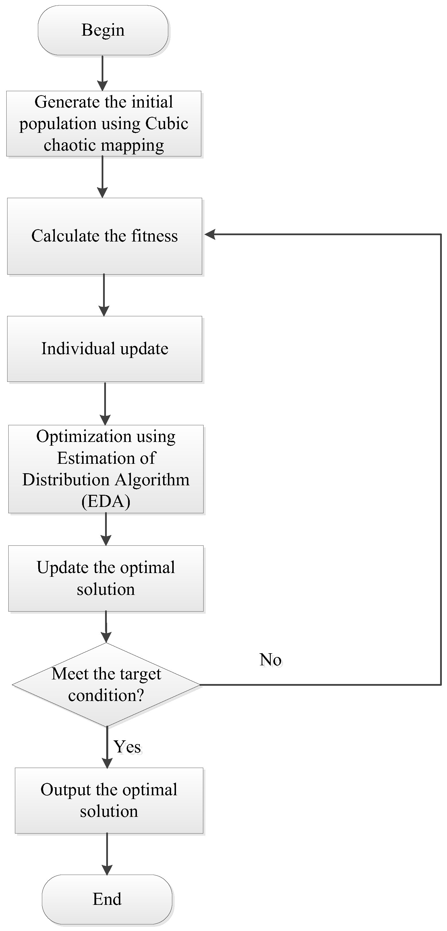
3.1. The Sparrow Search Algorithm Based on Chaotic Mapping and Estimation of Distribution Algorithm (EDA)

Table 3 presents the optimization strategies for the Chaotic Sparrow Search Algorithm.

Table 3. Optimization strategies for chaotic sparrow search algorithm.

Optimization Strategy	Description	Limitations
Adaptive Weight Strategy	Dynamically adjusts the weight of individuals’ position updates, enhancing exploration in early stages and exploitation in later stages.	Requires fine-tuning, which may increase computational complexity.
Mutation Strategy	Introduces random mutations similar to genetic algorithms, increasing population diversity and preventing early convergence.	Excessive mutation can lead to instability and impact convergence accuracy.
Multi-Strategy Cooperative Optimization	Combines multiple algorithm strategies (e.g., PSO, GA, DE) to enhance global search and convergence performance through synergy.	High algorithmic complexity; managing conflicts between different strategies can be challenging.
Levy Flight Strategy	Utilizes the Levy flight mechanism to allow individuals to perform long-distance jumps, enhancing global exploration capability.	Jump distances are hard to control and may lead to unstable search processes.
Adaptive Chaos Strategy	Dynamically adjusts chaotic parameters during the search, allowing different chaotic behaviors at various stages to balance exploration and exploitation.	Parameter selection can be complex and problem-dependent.

The workflow of the sparrow search algorithm based on Chaotic Mapping and Estimation of Distribution Algorithm (EDA) is shown in Figure 3.

Figure 3. Flowchart of sparrow search algorithm Based on Cubic Map and EDA.

(1)

Generate the initial population using the cubic chaotic map to determine the initial positions of the population, as described by the following equation:

$$x_i^0=L_b+\left(U_b-L_b\right)\cdot x_{chaotic}^i$$

(18)

where: $L_b,U_b$—the lower and upper boundaries of the solution space; $x_{chaotic}^i$—Chaotic sequence generated by the cubic chaotic map.

(2)

Fitness Calculation: For each individual in the initial population, calculate its fitness value and determine the position and fitness of the best individual in the population.

(3)

Iterative Population Update: Update the positions of explorers, followers, and scouts in the population according to the standard SSA update rules.

(4)

Optimization using EDA: Every five iterations, apply EDA for the secondary optimization of the current population. Construct a Gaussian probability model to generate new individuals, replacing underperforming ones. The formula is as follows:

$$P\left(x\right)={\displaystyle \frac{1}{\sqrt{(2\pi {)}^n|\Sigma |}}}\exp \left(-{\displaystyle \frac{1}{2}}(x-\mu {)}^T{\Sigma }^{-1}(x-\mu )\right)$$

(19)

where: μ—mean vector; $\Sigma$—covariance matrix.

The pseudocode for the sparrow search algorithm is shown in Table 4.

Table 4. Sparrow search algorithm based on cubic mapping and EDA.

The Framework of Sparrow Search Algorithm
input:
G: Maximum Number Of Iterations;
w: Number of Discoverers in Sparrow Population;
SD: Number of vigilantes in the sparrow population;
R2: warning value;
Establish an objective function $F\left(x\right)$,where $N$ $X=x\left(x_1,x_2,\cdots ,x_d\right)$, are initialized by cubic algorithm and relevant parameters are defined;
output: $x_{\mathrm{best}},f_g;$
1: while $t\le G;$
2: Sort the fitness values to find the current best individual and the current worst individual;
${3:R}_2=\mathrm{rand}\left(1\right);$
4: for $i=1:N^{\mathrm{*}}w;$
5: Update the position of individual sparrow discoverers using Equation (13);
6: end for;
7: for $i=\left(N^{\mathrm{*}}w+1\right):N;$
8: Use Equation (14) to update the position of individual sparrow joiners;
9: end for;
10: for $i=1:S{D}^{\mathrm{*}}N;$
11: Use Equation (15) to update the position of individual sparrow watchers;
12: Use EDA for optimization: construct a Gaussian probability model using Equation (31) to generate new individuals after every five iterations, replacing those with poor performance.
12: end for;
13: Obtain the latest global optimum;
14: $t=t+1;$
15: end while;
16: return $x_{\mathrm{best}},f_g$.

3.2. TESA-FBP Model Evaluation Process

The BP neural network suffers from a slow convergence speed and a tendency to become trapped in local optima. To address these issues, a fractional-order BP neural network evaluation model was developed, which achieves better optimization results compared to traditional BP neural networks. The model is further enhanced by employing a Chaotic Sparrow Search Algorithm, resulting in the TESA-FBP prediction model. The core concept of this model involves using the TESA algorithm to repeatedly adjust the initial weights and thresholds of the fractional-order BP neural network to improve the model’s evaluation accuracy.

The evaluation process of the TESA-FBP model is as follows:

Step 1: Initialize Population and Parameter Setting

Generate the initial population using the cubic mapping strategy to ensure diversity and even distribution. Set the number of iterations for the algorithm and determine the ratio of predators to joiners.

Step 2: Calculate Fitness Values

Compute the fitness value for each individual (i.e., sparrow) in the initial population. Rank the population based on fitness values to identify the best and worst individuals.

Step 3: Update Sparrow Positions

Update the positions of discoverers, joiners, and sentinel sparrows according to the fitness ranking.

Step 4: Position Comparison and Update

In each iteration, compare the fitness values of the new positions with those from the previous iteration. If the new position has a better fitness value, update the sparrow position; otherwise, retain the original position. Repeat this process until the preset conditions are met (e.g., reaching the maximum number of iterations or achieving a fitness value threshold) to obtain the global optimum individual and best fitness value.

Step 5: Apply EDA Optimization

After every five iterations, construct a Gaussian probability model to generate new individuals, replacing those with poorer performance.

Step 6: Update the Optimal Solution

Compare the fitness values of the current population and update the global optimal solution. Continue executing Step 2 until the termination condition is met.

Step 7: Apply Optimal Solution to fractional-order BP neural network

Convert the global optimal individual into weight values for the fractional-order BP neural network. The global optimal solution also serves as the threshold value for the fractional-order BP neural network.

Step 8: Termination and Output

When one of the stopping conditions is satisfied, stop the training process and output the current neural network’s weights, thresholds, and corresponding prediction results. If the stopping conditions are not met, continue the training process for the fractional-order BP neural network.

3.3. Experimental Analysis

3.3.1. Selection of Experimental Data and Evaluation Metrics

The data for the network security situation awareness system comes from the naval weaponry preliminary research project, specifically the electronic information system for maritime battlefields, making the data highly sensitive. To validate the model’s effectiveness, publicly available network security situation data from the National Computer Network Emergency Response Technical Team/Coordination Center of China (CNCERT/CC) is used as experimental data. These statistical data mainly come from the security situation weekly reports regularly published on the CNCERT/CC website. The reports cover five major categories of security incidents: the number of hosts infected by viruses, number of websites defaced, number of websites implanted with backdoors, number of phishing websites, and number of new security vulnerabilities. These five categories are the main factors affecting the situation assessment level, are independent of each other, and have obtainable relevant data, making them operable and suitable for indicator selection. Thus, these five categories of incidents are selected as indicators for assessing the network security situation. For a more efficient data analysis, the five security situation assessment levels provided by CNCERT/CC are converted into numerical levels, as shown in Table 5.

Table 5. Five levels of network security situation.

Excellent	Good	Secondary	Poor	Dangerous
5	4	3	2	1

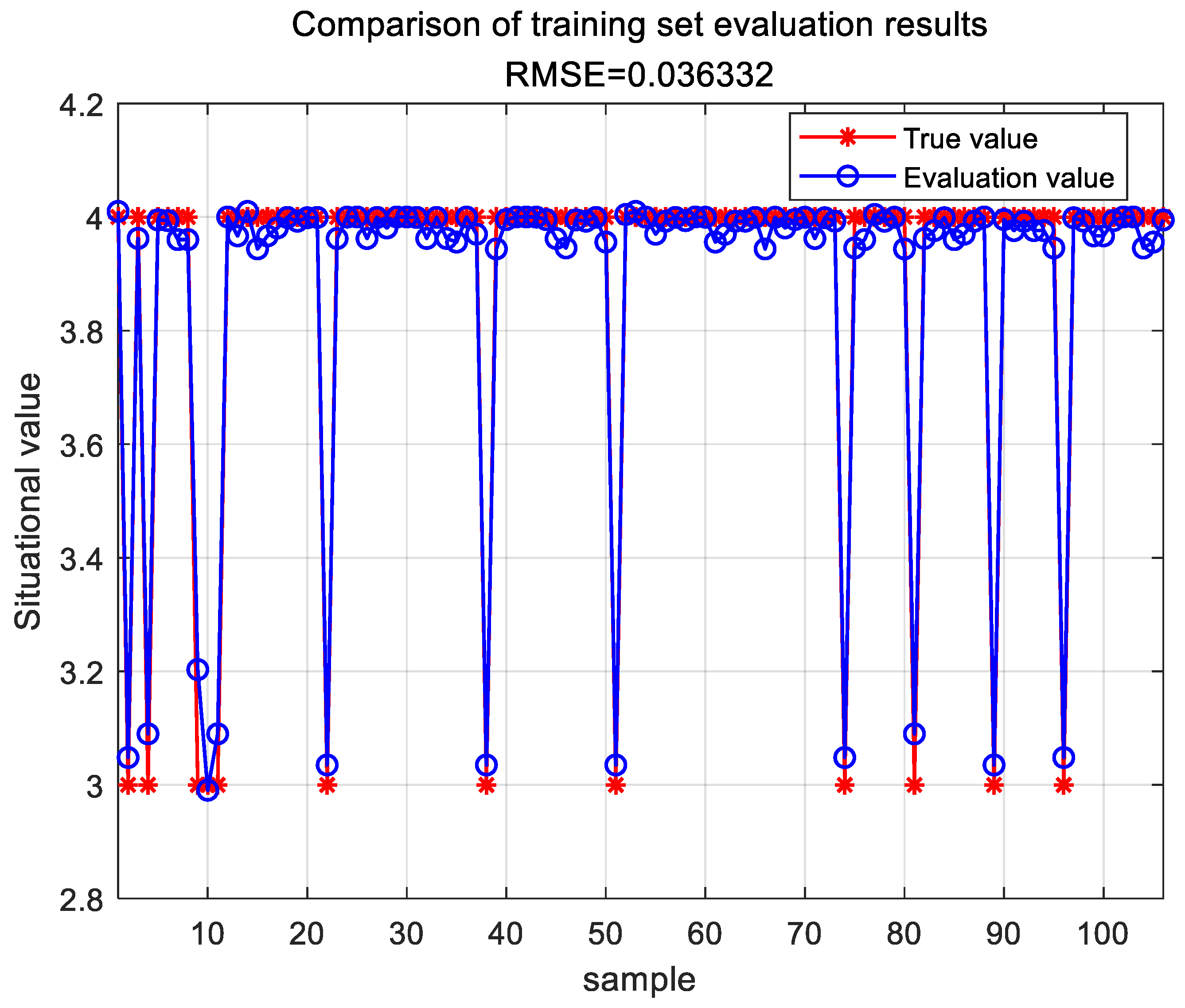
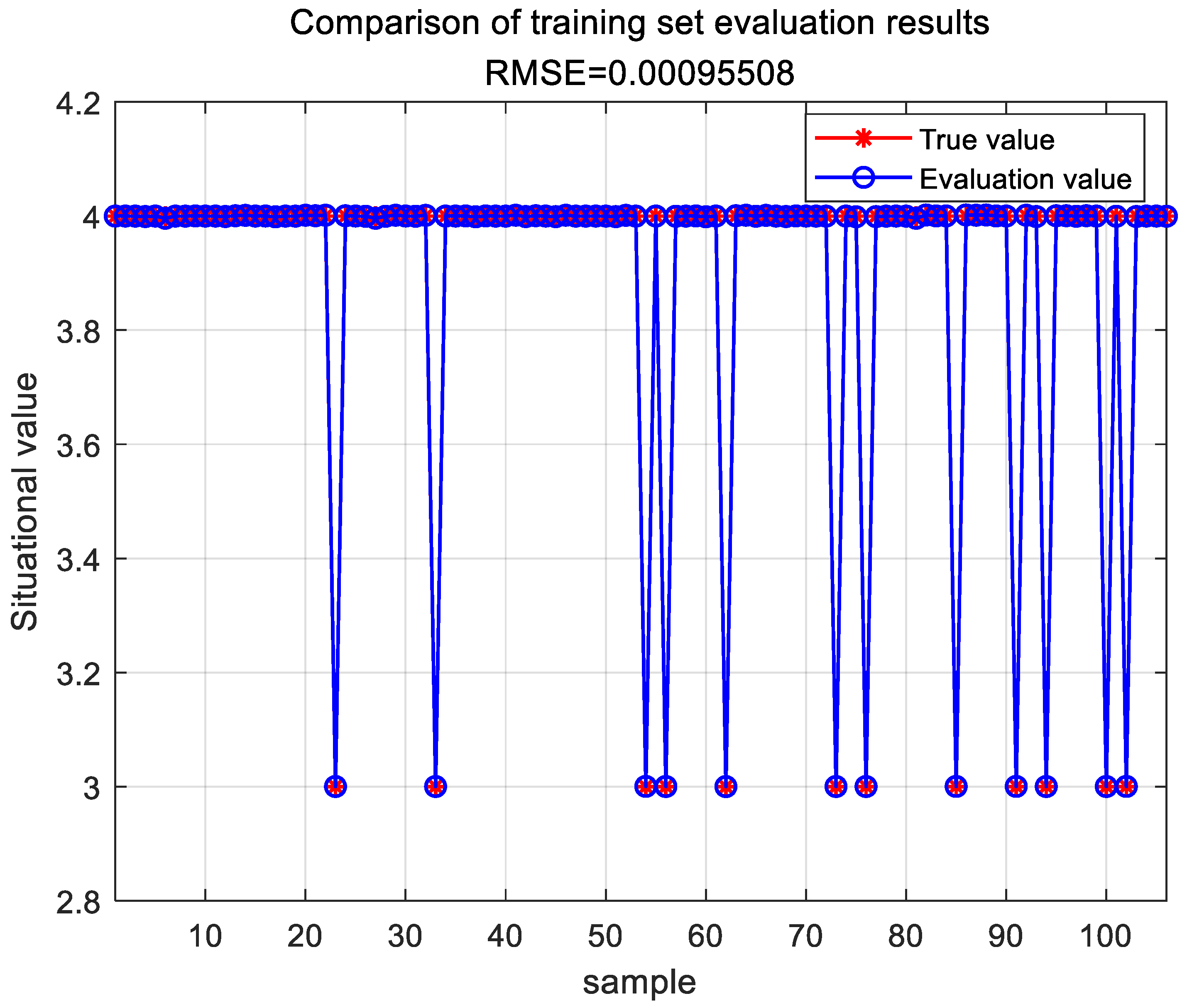
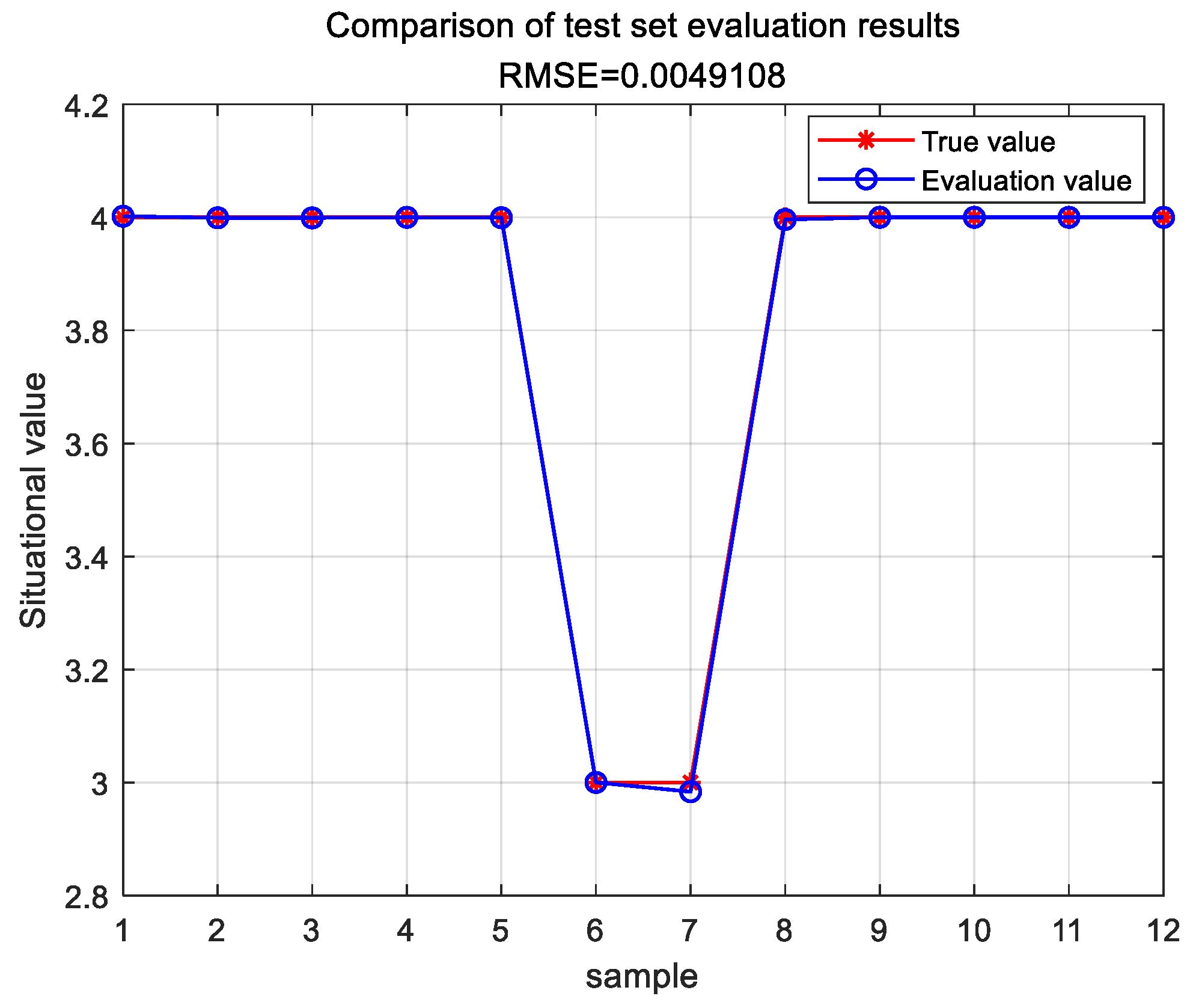
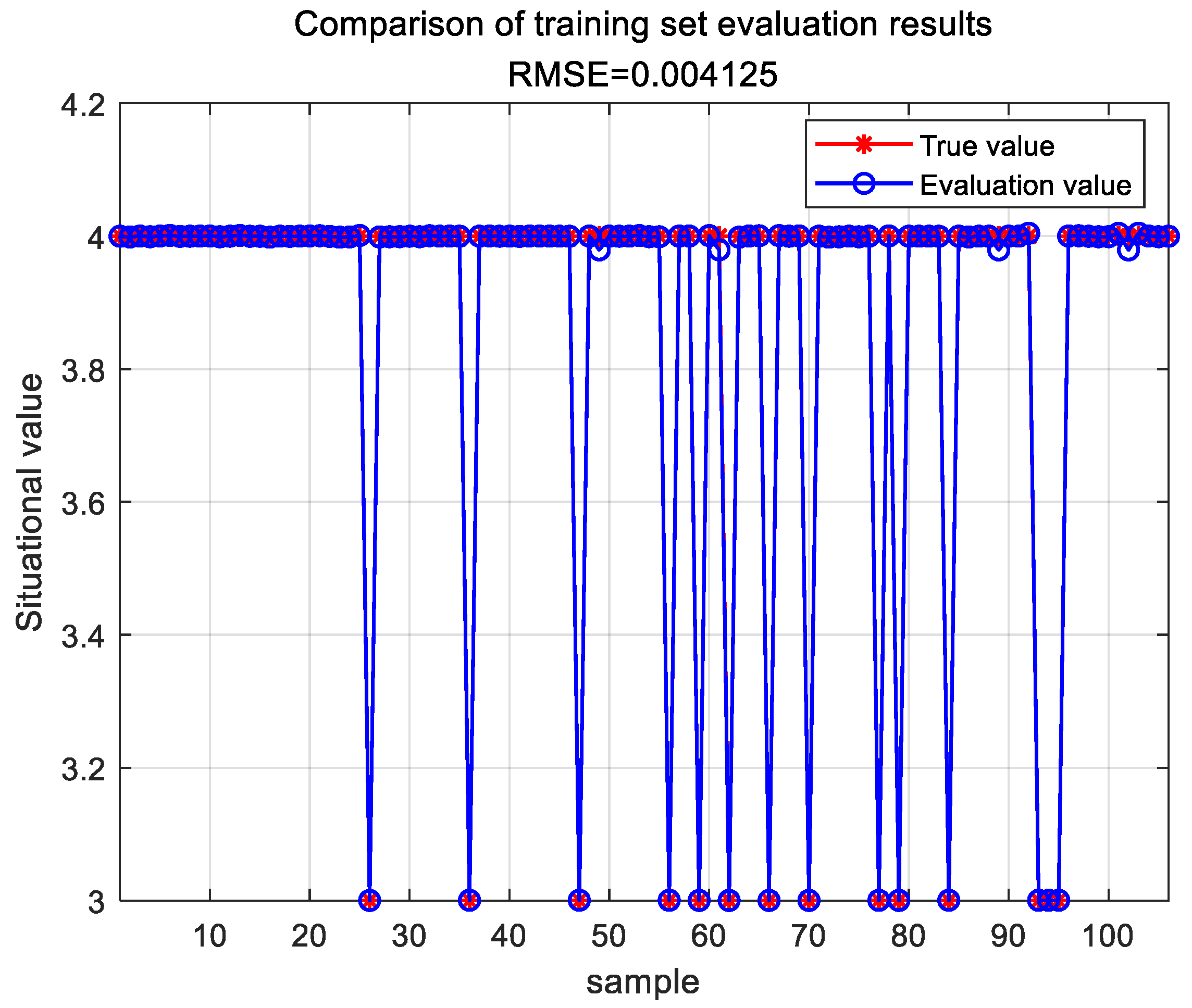
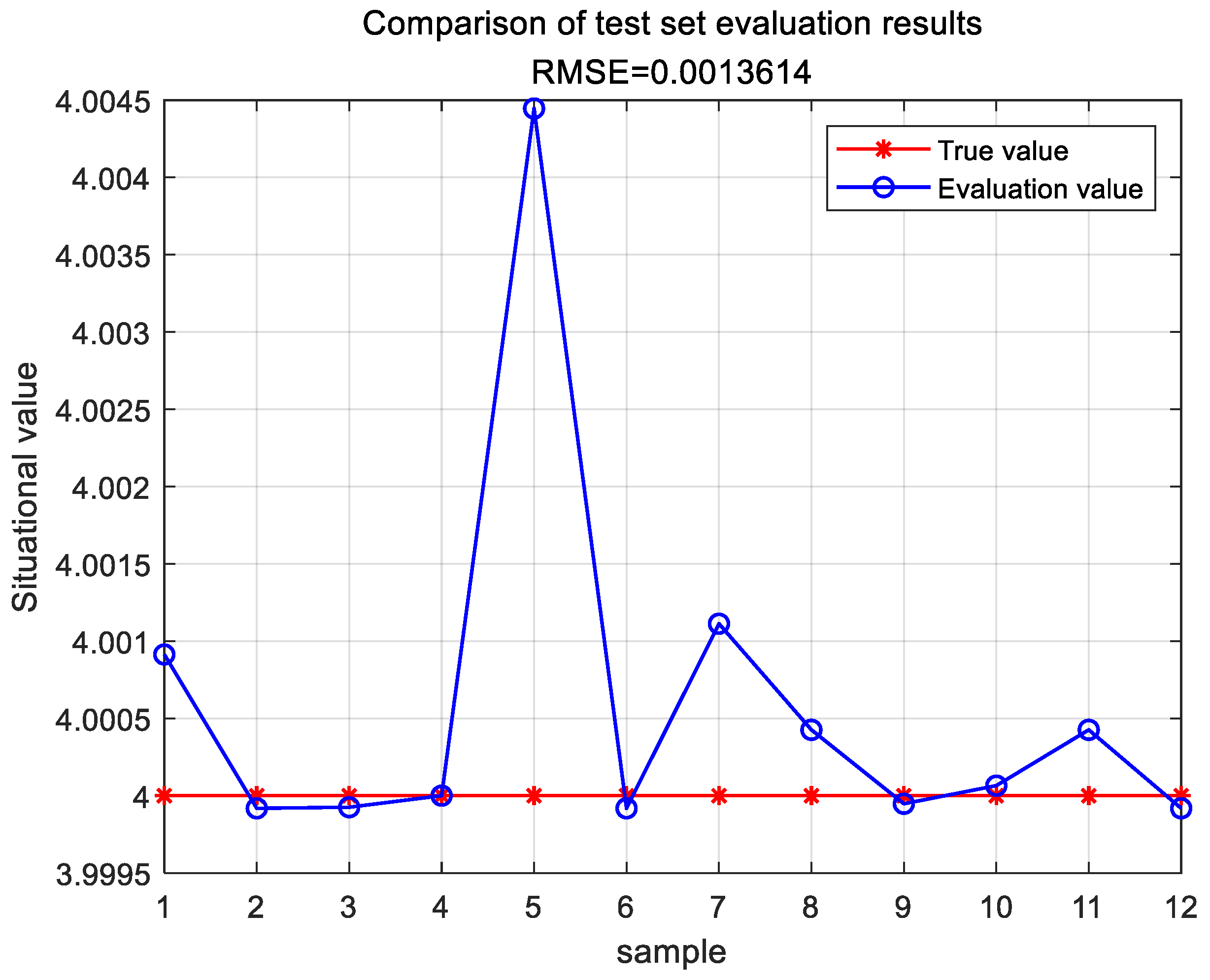
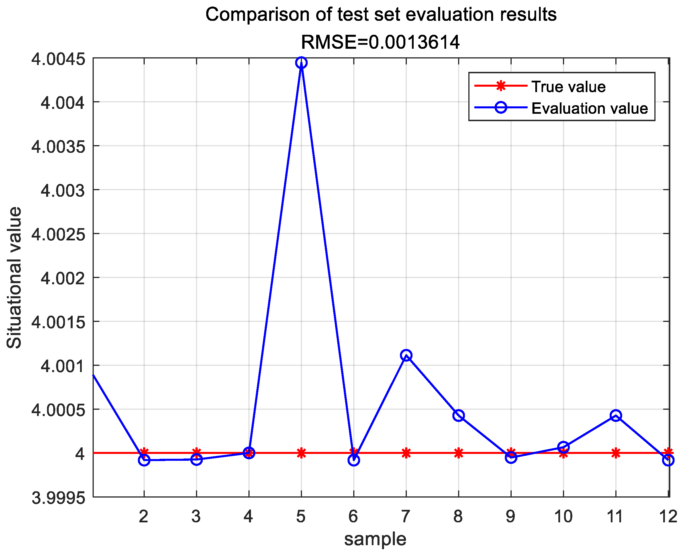
3.3.2. Evaluation Model Comparison

(1) BP Neural Network Based on Simulated Annealing and Particle Swarm Optimization (SA-PSO-BP) Evaluation Model

A BP neural network employing simulated annealing and particle swarm optimization was trained and then used for situation assessment. The evaluation results for the training set are shown in Figure 4.

Figure 4. Evaluation results of the SA-PSO-BP training set.

The evaluation results for the test set are shown in Figure 5.

Figure 5. Evaluation results of the SA-PSO-BP test set.

The error between the situation evaluation results obtained through the SA-PSO-BP model and the actual situation values is shown in Table 6.

Table 6. Comparison of assessment results of the SA-PSO-BP model situation.

Sample	Actual Value	Evaluation Value	Absolute Error
1	3	3.048	0.048
2	4	3.995	0.005
3	4	4	0
4	4	3.993	0.007
5	4	4.005	0.005
6	4	3.981	0.019
7	4	3.998	0.002
8	4	4	0
9	4	4.01	0.01
10	3	3.09	0.09
11	4	3.993	0.007
12	4	4.005	0.005

(2) Evaluation Model Based on BP Neural Network Optimized by D-S Evidence [37].

Theory (D-S BP) The parameters of the BP neural network were optimized using the D-S evidence theory. After training with the sample data, the GA-BP evaluation model was successfully constructed. This model was then used to evaluate and analyze 12 sample data points. The evaluation results of the training set are shown in Figure 6.

Figure 6. Evaluation results of the D-S-BP training set.

The evaluation results of the test set are shown in Figure 7.

Figure 7. Evaluation results of the D-S-BP test set.

The error between the situational assessment results obtained through the D-S-BP model evaluation and the actual situational values is shown in Table 7.

Table 7. Comparison of D-S-BP model situation evaluation results.

Sample	Actual Value	Evaluation Value	Absolute Error
1	4	4.001	0.001
2	4	4	0
3	4	4	0
4	4	4	0
5	4	4.004	0.004
6	4	4	0
7	4	4.001	0.001
8	4	4	0
9	4	4	0
10	4	4	0
11	4	4	0
12	4	4	0

(3) Genetic Algorithm Based Deep Neural Network (GA-DNN) Evaluation Model [38].

The evaluation model was successfully constructed using the GA-DNN algorithm based on Euclidean distance. Subsequently, this model was utilized for the evaluation analysis of the 12 sample datasets. The evaluation results of the training set are depicted in Figure 8.

Figure 8. Evaluation results of the GA-DNN training set.

The evaluation results of the test set are shown in Figure 9.

Figure 9. Evaluation results of the GA-DNN test set.

Through the evaluation of the GA-DNN model, the calculated error between the situation assessment results and the actual situation values is presented in Table 8.

Table 8. Comparison of GA-DNN Model Situation Evaluation Results.

Sample	Actual Value	Evaluation Value	Absolute Error
1	4	4.002	0.002
2	4	3.999	0.001
3	4	3.999	0.001
4	4	4	0
5	4	3.999	0.001
6	3	3	0
7	3	2.984	0.016
8	4	3.996	0.004
9	4	4	0
10	4	4	0
11	4	4	0
12	4	4	0

(4) The Evaluation Model of TESA-FBP Based on chaotic sparrow search algorithm Optimization

The parameters of the BP neural network were optimized using a Chaotic Sparrow Search Algorithm. Through training on the sample data, the TESA-FBP evaluation model was successfully constructed. This model was then utilized to effectively evaluate the 12 sample datasets, with the assessment results of the training set shown in Figure 10.

Figure 10. Evaluation results of the TESA-FBP training set.

The evaluation results of the test set are shown in Figure 11.

Figure 11. Evaluation results of the TESA-FBP test set.

Through the evaluation computation of the TESA-FBP model, the error between the situational assessment results and the actual situational values is depicted in Table 9.

Table 9. Comparison of evaluation results of the TESA-FBP model situation.

Sample	Actual Value	Evaluation Value	Absolute Error
1	4	4.001	0.001
2	4	4	0
3	4	4	0
4	4	4	0
5	4	4.005	0.005
6	4	4	0
7	4	4.001	0.001
8	4	4	0
9	4	4	0
10	4	4	0
11	4	4	0
12	4	4	0

This section may be divided into subheadings. It should provide a concise and precise description of the experimental results and their interpretation, as well as the experimental conclusions that can be drawn.

4. Discussion

This section introduces a network security situational assessment method based on the research topic of naval weaponry and equipment—the maritime electronic information system, which stipulates a performance requirement that the assessment delay must not exceed 20 s. Considering the applicability of BP neural networks to complex systems and their superior performance over deep learning algorithms with fewer input variables while meeting the performance requirements and accuracy of the assessment, optimizations were performed to address the slow convergence, poor stability, and tendency to fall into the local minima of traditional BP neural networks. The following two improvements were applied to the BP neural network using the fractional-order TESA-FBP algorithm:

To ensure that the sparrow algorithm avoids premature convergence and exhibits superior global search performance, the cubic chaotic optimization algorithm was employed to enhance population diversity. This approach enables the sparrow algorithm to achieve better diversity and global coverage in the initial stage. Due to the random properties of chaotic elements, they can enrich the initial dataset of the SSA algorithm, thus improving its global search efficiency. The cubic chaotic mapping operator, widely used for generating consistent chaotic sequences within the range [0, 1], offers a relatively high iteration rate. Consequently, the cubic chaotic mapping function, characterized by uniform distribution, unpredictability, irreproducibility, and thoroughness, was introduced. Using cubic chaotic mapping values to represent the initial positions of the population not only maintains the diversity of the sparrow search algorithm but also increases the likelihood of finding the globally optimal result, thereby accelerating the search rate and enhancing search efficiency. The introduction of chaotic variables significantly improves the global search capability, reduces the occurrence of local optima, and accelerates the convergence speed, thus ensuring good global convergence.

During the training of the neural network model, fractional-order improvements were applied to the BP neural network. The memory and non-local properties of the fractional order partially address the issues of slow convergence and long training times inherent in BP neural networks. By continuously adjusting the weights and constraints of each layer, this method reduces the deviation of the final output from the preset target value. This approach effectively mitigates the reduction in diversity and the local optimum problems associated with the increase in iteration counts of the sparrow search algorithm, thereby improving the accuracy, speed, and stability of the search algorithm.

The comparison results of the Mean Absolute Error (MAE) and the Root Mean Square Error (RMSE) for the evaluation results of the three model algorithms are shown in Table 10 and Table 11, respectively.

Table 10. MAE of three model.

Evaluation Model	MAE
SA-PSO-BP	0.0165
DS-BP	0.002083
GA-DNN	0.001065
TESA-FBP	0.000583

Table 11. RMSE of three model.

Evaluation Model	RMSE
	Train Data (90%)	Test Data (10%)
SA-PSO-BP	0.036332	0.036394
DS-BP	0.00095508	0.0049108
GA-DNN	0.00654654	0.0072345
TESA-FBP	0.004125	0.0013614

Based on the comparison results in Table 8 and Table 9, it is evident that the network security situational assessment results obtained using the TESA-FBP model proposed in this chapter are the lowest in terms of the performance metrics MAE and RMSE compared to the SA-PSO-BP, DS-BP, and GA-DNN models. Experimental evidence demonstrates that the TESA-FBP model effectively enhances both the accuracy and efficiency of network security situational assessments.

The proposed network security situational awareness assessment model utilizes public data provided by the National Emergency Response Center as experimental data, using five types of events as primary evaluation indicators. Based on these primary indicators, the model achieves good evaluation accuracy and delay. In more complex network security systems, it is often necessary to construct multilevel evaluation indicators. Future research could further explore ways to improve the accuracy and convergence speed of the algorithm model under a multilevel evaluation indicator system.

5. Conclusions

The advantages of the network security situation assessment model proposed in this article are as follows:

(1)

High Adaptability: The chaotic sparrow algorithm enhances the diversity and global optimization capability of the search process through chaotic mapping, thereby improving the model’s adaptability in complex environments.

(2)

High Optimization Efficiency: EDA (Estimation of Distribution Algorithm) effectively utilizes information from historical data distributions to guide the search process, allowing the model to converge more quickly in large-scale data and complex network structures.

(3)

Model Stability: The fractional-order BP (Backpropagation) model increases the network’s memory capacity and robustness by incorporating fractional-order calculus, leading to greater stability when dealing with variations in complex network environments.

(4)

Computational Complexity Management: The combination of chaotic sparrow optimization and EDA effectively manages computational complexity, maintaining high efficiency even when handling large-scale networks.

Performance tests of the algorithm convergence speed and global optimization capability were conducted using public situational data from the National Internet Emergency Center. The TESA-FBP evaluation model was compared with the recently proposed SA-PSO-BP, DS-BP, and GA-DNN models using the performance metrics MAE and RMSE. Experimental results demonstrate that the TESA-FBP model proposed in this chapter achieves higher prediction accuracy, validating its precision and effectiveness.

References

- Talebi, S.P.; Werner, S.; Li, S.; Mandic, D.P. Tracking dynamic systems in α stable environments. In Proceedings of the IEEE International Conference on Acoustics, Speech and Signal Processing, Brighton, UK, 12–17 May 2019; pp. 4853–4857. [Google Scholar]
- Bai, L.; An, Y.; Sun, Y. Measurement of project portfolio benefits with a GA-BP neural network group. IEEE Trans. Eng. Manag. 2023, 71, 4737–4749. [Google Scholar] [CrossRef]
- Chaudhary, N.I.; Zubair, S.; Raja, M.A.Z. A new computing approach for power signal modeling using fractional adaptive algorithms. ISA Trans. 2017, 68, 189 202. [Google Scholar] [CrossRef] [PubMed]
- Gorenflo, R.; Mainardi, F. Fractional Calculus: Integral and Differential Equations of Fractional Order; Springer: Berlin/Heidelberg, Germany, 1997. [Google Scholar]
- Sabatier, J.; Agrawal, O.P.; Machado, J.T. Advances in Fractional Calculus; Springer: Berlin/Heidelberg, Germany, 2007. [Google Scholar]
- Machado, J.T.; Kiryakova, V.; Mainardi, F. Recent history of fractional calculus. Commu Nications Nonlinear Sci. Numer. Simul. 2011, 16, 1140–1153. [Google Scholar] [CrossRef]
- Alsaedi, A.; Ahmad, B.; Kirane, M. A survey of useful inequalities in fractional calculus. Fract. Calc. Appl. Anal. 2017, 20, 574–594. [Google Scholar] [CrossRef]
- Luchko, Y. Fractional derivatives and the fundamental theorem of fractional calculus. Fract. Calc. Appl. Anal. 2020, 23, 939–966. [Google Scholar] [CrossRef]
- Hamamci, S.E. An algorithm for stabilization of fractional order time delay systems using fractional order pid controllers. IEEE Trans. Autom. Control. 2007, 52, 1964–1969. [Google Scholar] [CrossRef]
- Kumar, A.; Pan, S. Design of fractional order pid controller for load frequency control system with communication delay. ISA Trans. 2022, 129, 138–149. [Google Scholar] [CrossRef]
- Pu, Y.F.; Zhou, J.L.; Yuan, X. Fractional differential mask: A fractional differential based approach for multiscale texture enhancement. IEEE Trans. Image Process. 2010, 19, 491–511. [Google Scholar]
- Pu, Y.F.; Siarry, P.; Chatterjee, A.; Wang, Z.N.; Yi, Z.; Liu, Y.G.; Zhou, J.L.; Wang, Y. A fractional order variational framework for retinex: Fractional order partial differential equation based formulation for multi scale nonlocal contrast en hancement with texture preserving. IEEE Trans. Image Process. 2018, 27, 1214–1229. [Google Scholar] [CrossRef]
- Wang, Q.; Ma, J.; Yu, S.; Tan, L. Noise detection and image denoising based on fractional calculus. Chaos Solitons Fractals 2020, 131, 109463. [Google Scholar] [CrossRef]
- Munkhammar, J. Chaos in a fractional order logistic map. Fract. Calc. Appl. Anal. 2013, 16, 511–519. [Google Scholar] [CrossRef]
- Wu, G.C.; Baleanu, D.; Zeng, S.D. Discrete chaos in fractional sine and standard maps. Phys. Lett. A 2014, 378, 484–487. [Google Scholar] [CrossRef]
- Wang, S.; Zhu, H.; Wu, M.; Zhang, W. Active disturbance rejection decoupling control for three-degree-of-freedom six-pole active magnetic bearing based on BP neural network. IEEE Trans. Appl. Supercond. 2020, 30, 1–5. [Google Scholar] [CrossRef]
- Liu, X.; Zhou, Y.; Wang, Z.; Chen, X. A BP neural network-based communication blind signal detection method with cyber-physical-social systems. IEEE Access 2018, 6, 43920–43935. [Google Scholar] [CrossRef]
- Tian, L.; Noore, A. Short-term load forecasting using optimized neural network with genetic algorithm. In Proceedings of the 2004 International Conference on Probabilistic Methods Applied to Power Systems, Ames, IA, USA, 12–16 September 2004; pp. 135–140. [Google Scholar]
- Dam, M.; Saraf, D.N. Design of neural networks using genetic algorithm for on-line property estimation of crude fractionator products. Comput. Chem. Eng. 2006, 30, 722–729. [Google Scholar] [CrossRef]
- Panda, S.S.; Ames, D.P.; Panigrahi, S. Application of vegetation indices for agricultural crop yield prediction using neural network techniques. Remote Sens. 2010, 2, 673–696. [Google Scholar] [CrossRef]
- Zuogong, W.; Huiyang, L.I.; Yuanhua, J.I.A. A neural network model for expressway investment risk evaluation and its application. J. Transp. Syst. Eng. Inf. Technol. 2013, 13, 94–99. [Google Scholar]
- Wang, W.; Tang, R.; Li, C.; Liu, P.; Luo, L. A BP neural network model optimized by mind evolutionary algorithm for predicting the ocean wave heights. Ocean. Eng. 2018, 162, 98–107. [Google Scholar] [CrossRef]
- Tan, X.; Ji, Z.; Zhang, Y. Non-invasive continuous blood pressure measurement based on mean impact value method, BP neural network, and genetic algorithm. Technol. Health Care 2018, 26 (Suppl. S1), 87–101. [Google Scholar] [CrossRef]
- Mamat, T.; Jumaway, M.; Zhang, X.; Hassan, M. Research on impact factors of agricultural mechanization development level based on BP neural network. J. Agric. Mech. Res. 2018, 40, 21–25. [Google Scholar]
- Chen, W. BP Neural Network-Based Evaluation Method for Enterprise Comprehensive Performance. Math. Probl. Eng. 2022, 2022, 1–11. [Google Scholar]
- Liu, J.; He, X.; Huang, H.; Yang, J.; Dai, J.; Shi, X.; Xue, F.; Rabczuk, T. Predicting gas flow rate in fractured shale reservoirs using discrete fracture model and GA-BP neural network method. Eng. Anal. Bound. Elem. 2024, 159, 315–330. [Google Scholar] [CrossRef]
- Zhou, J.; Lin, H.; Li, S.; Jin, H.; Zhao, B.; Liu, S. Leakage diagnosis and localization of the gas extraction pipeline based on SA-PSO BP neural network. Reliab. Eng. Syst. Saf. 2023, 232, 109051. [Google Scholar] [CrossRef]
- Li, X.; Jia, C.; Zhu, X.; Zhao, H.; Gao, J. Investigation on the deformation mechanism of the full-section tunnel excavation in the complex geological environment based on the PSO-BP neural network. Environ. Earth Sci. 2023, 82, 326. [Google Scholar] [CrossRef]
- Tutueva, A.V.; Nepomuceno, E.G.; Karimov, A.I.; Andreev, V.S.; Butusov, D.N. Adaptive chaotic maps and their application to pseudo-random numbers generation. Chaos Solitons Fractals 2020, 133, 109615. [Google Scholar] [CrossRef]
- Shahna, K.U. Novel chaos based cryptosystem using four-dimensional hyper chaotic map with efficient permutation and substitution techniques. Chaos Solitons Fractals 2023, 170, 113383. [Google Scholar] [CrossRef]
- Wang, Y.; Liu, H.; Ding, G.; Tu, L. Adaptive chimp optimization algorithm with chaotic map for global numerical optimization problems. J. Supercomput. 2023, 79, 6507–6537. [Google Scholar] [CrossRef]
- Aydemir, S.B. A novel arithmetic optimization algorithm based on chaotic maps for global optimization. Evol. Intell. 2023, 16, 981–996. [Google Scholar] [CrossRef]
- Mehmood, K.; Chaudhary, N.I.; Khan, Z.A.; Cheema, K.M.; Raja, M.A.Z.; Shu, C.M. Novel knacks of chaotic maps with Archimedes optimization paradigm for nonlinear ARX model identification with key term separation. Chaos Solitons Fractals 2023, 175, 114028. [Google Scholar] [CrossRef]
- Mehmood, K.; Chaudhary, N.I.; Khan, Z.A.; Cheema, K.M.; Zahoor Raja, M.A. Atomic physics-inspired atom search optimization heuristics integrated with chaotic maps for identification of electro-hydraulic actuator systems. Mod. Phys. Lett. B 2024, 38, 2450308. [Google Scholar] [CrossRef]
- Aguiar, B.; González, T.; Bernal, M. A way to exploit the fractional stability domain for robust chaos suppression and synchronization via LMIs. IEEE Trans. Autom. Control. 2015, 61, 2796–2807. [Google Scholar] [CrossRef]
- Olusola, O.I.; Vincent, E.; Njah, A.N.; Ali, E. Control and synchronization of chaos in biological systems via backsteping design. Int. J. Nonlinear Sci. 2011, 11, 121–128. [Google Scholar]
- Yin, K.; Yang, Y.; Yang, J.; Yao, C. A network security situation assessment model based on BP neural network optimized by D-S evidence theory. J. Phys. Conf. Ser. 2022, 2258, 012039. [Google Scholar] [CrossRef]
- Rezaeian, N.; Gurina, R.; Saltykova, O.A.; Hezla, L.; Nohurov, M.; Reza Kashyzadeh, K. Novel GA-Based DNN Architecture for Identifying the Failure Mode with High Accuracy and Analyzing Its Effects on the System. Appl. Sci. 2024, 14, 3354. [Google Scholar] [CrossRef]
Disclaimer/Publisher’s Note: The statements, opinions and data contained in all publications are solely those of the individual author(s) and contributor(s) and not of MDPI and/or the editor(s). MDPI and/or the editor(s) disclaim responsibility for any injury to people or property resulting from any ideas, methods, instructions or products referred to in the content. |
© 2024 by the authors. Licensee MDPI, Basel, Switzerland. This article is an open access article distributed under the terms and conditions of the Creative Commons Attribution (CC BY) license (https://creativecommons.org/licenses/by/4.0/).