1. Introduction
Due to their significance in mathematical analysis, functional analysis, physics, and other subjects, special functions are those functions that have generally established names and notions. Although there is not a single formal definition for all these mathematical functions, the list includes several generally recognized as special. Elementary functions, particularly trigonometric functions, are considered special functions. With the help of Gauss, Jacobi, Klein, and many others, the theory was largely developed in the nineteenth century. Special functions have been employed for ages due to their extraordinary qualities. For instance, trigonometric functions have been used for over a thousand years due to their numerous astronomical applications. Since the beginning of the twentieth century, disciplines including topology, algebra, differential equations, real and functional analysis, and special functions have taken center stage. Nevertheless, a book written by G.N. Watson [
1] was published then and is a crucial contribution to the theory, particularly in the context of asymptotic expansions of Bessel functions. As a classic today, special functions such as hypergeometric and Bessel functions are often utilized in statistics, probability, mathematical physics, and engineering disciplines due to their amazing features. Because of this, Paul Tur’an, a Hungarian mathematician, thought the term “special functions” was misleading and that the more accurate term would be useful functions.
A special function known as the Mittag-Leffler (ML) function arises naturally in the solution integral equations of fractional order and is acclaimed as the queen function of fractional calculus. The increased interest in this function over the past few years is mostly because of its strong connection to fractional calculus and, in particular, to fractional difficulties that arise in applications. In recent decades, the ML function and its various extensions have been used successfully to solve various problems in physics, engineering, chemistry, biology, and other practical disciplines, increasing its visibility among scientists. The study of these functions’ analytical features has generated a sizable body of literature; many authors have looked into these functions from a mathematical perspective [
2].
The ML function
of two parameters, which can be regarded as a simple extension of the classical ML function, is provided as
The Mittag-Leffler functions described in (1) originally appeared in Wiman’s [
3] work. These functions were later investigated by Agarwal [
4].
In 1949, Russian researcher Yuriy Nicholaevich Rabotnov, who carried out work in solid mechanics consisting of a broad range of topics, including creep theory, plasticity, heredity mechanics, nonelastic stability, failure mechanics, shell theory, and composites, introduced a function by utilizing
. Today, it is recognized in his name as the Rabotnov fractional exponential function [
5] or simply Rabotnov function. It is provided as
It is clear that this series will converge at any argument value. Note that it becomes the typical exponential
for
. The following is a possible way to express the relationship between
and
:
The fact that is a fractional extension of the fundamental functions is another significant and intriguing aspect of these functions. That is, , , ,
The Rabotnov fractional exponential function is utilized by Yang et al. [
6] to introduce a fractional derivative with a nonsingular kernel.
Definition 1. The following represents the fractional derivative with Rabotnov exponential kernel of the function , of order swith and The following definition presents the integral representation of the fractional derivative with a Rabotnov exponential kernel.
Definition 2. The fractional integral with Rabotnov exponential kernel of the function , of order s is provided bywith and Special functions like hypergeometric, Bessel, and Mittag-Leffler play a significant role in function theory. The solution of the classic Bieberbach conjecture may be the most well-known use of these functions in the theory. Due to the unexpected application of hypergeometric functions by L. de Branges, there has been much interest in the geometric characteristics of generalized, Kummer, and Gauss hypergeometric functions and certain other functions in recent years. Although the geometric characteristics of these functions are intriguing in and of themselves, they have proven useful in numerous other function theory problems.
The geometric characteristics and uses of the function
and some related functions have recently piqued scholars’ curiosity. It is natural to provide some recent developments on the geometric properties of ML functions as the function
can be written in the form of
Some geometrical characteristics of Mittag-Leffler functions were discussed by Bansal [
7]. Partial sums of these functions were the focus of Raducanu’s [
8] work. Noreen et al. [
9,
10,
11] studied the geometric properties of this function extensively, whereas Das and Mehrez [
12] improved the results of Noreen et al. Srivastava et al. [
13] studied a three-parameter Mittag-Leffler function.
The upcoming sections are organized as follows:
Section 2 starts with some basic definitions of concepts of geometric functions theory and Hardy spaces, followed by some important lemmas that are useful in our discussions in the next sections. Lastly, we provide brief discussions pertaining to the normalized form of Rabotnov functions and some recent work on the geometric properties of this function. In
Section 3, we state and prove the main theorems related to the study of geometric properties of the Rabotnov function along with examples. In
Section 4, Hardy spaces are demonstrated, along with final remarks.
2. Preliminaries
The following well-known definitions are required for our study.
Denote by
, the class of analytic functions in
and
a subclass of
, which contains functions
f of the form
Let
stand for the class of all functions in
that contains univalent (one-to-one) functions in
. Consider
f,
. Then,
f is subordinated by
g and symbolically written as
if there exists a function
w known as Schwarz function that has the property that it is an analytic self map in
with
such that
Additionally, if
g is one-to-one in
, then the analogous relation shown below holds:
Let
be analytic in
and provided by (2) and
is analytic in
. Then, convolution (Hadamard product) of these functions is provided by
Let and be subclasses of , which, respectively, represent strongly starlike and convex functions of order .
Definition 3. A function , if and only if Definition 4. A function if and only if It is noted that and where and are familiar classes of starlike and convex functions, respectively. Similarly, and denote the classes of stalike and convex functions of order We define these as follows:
Definition 5. A function if and only if Definition 6. A function if and only if and Rosy et al. [
14] introduced a subclass of
. It is denoted by
.
Definition 7. A function is in if and only if We denote by a class of uniformly convex functions in .
Definition 8. A function f is in if and only if Definition 9 ([
15])
. The classes and are defined as and where , For the classes and are denoted by and , respectively. Also, for and we have the classes and .
Let
represent the space of functions on
, which are bounded in
. This set represents a Banach algebra with norm provided by
The space of all those functions
such that
admits a harmonic majorant is denoted by
. If the norm of
f is given to be
p-th root of the least harmonic majorant of
for some fixed
, then it is a Banach space. Another definition of norm is provided as follows. Let
, set
Then,
if
is bounded for all
We see that
From [
16], if
in
, then
Our aim in this study is to determine sufficiency criterion for Rabotnov function to be uniformly convex, strongly starlike, strongly convex, and demonstrate Hardy spaces of Rabotnov function.
The Rabotnov function
is not in class
; therefore, consider the transformation
such that
provided by
The geometric properties of
have recently been discussed by Eker and Ece [
17] and Eker et al. [
18]. Partial sums of generalized function of
have been studied by Frasin [
19]. Amourah et al. [
20] have studied certain subclasses of bi-univalent functions involving the function
Deniz and Kazimoglu [
21] studied Hardy spaces by using a different technique for this function.
In this study, we restrict ourselves such that s and are real.
We require the following results for our study.
Lemma 1 ([
22])
. If , and of the form (2), then Lemma 2 ([
17])
. Let and . Then, Lemma 3 ([
23])
. Let g and be analytic functions in with Let g be univalent and convex in and in . Then, Lemma 4 ([
24])
. If satisfies then Lemma 5 ([
25])
. where with and γ has the best possible value. Lemma 6 ([
26])
. For and we have or equivalently Lemma 7 ([
27])
. If the function f, convex of order γ, where is not of the form where m, and then the following claims are true: - (i)
There exists such that
- (ii)
If then there exists such that
- (iii)
If then
3. Main Results
Theorem 1. If and and then whereand Proof. By using a result due to [
17], we have
For
and from (4)
we concluded that
For
by using Lemma 3, with
and
we obtain
By using (5) and (6)
we obtain
Which implies that for □
In the following, we provide a few examples by taking particular values of s and
Example 1. The function where
The function where
The function where
The function where
Theorem 2. If and and then wherewith Proof. For
and from (7)
we concluded that
For
by using Lemma 3 with
and
we obtain
By using (8) and (9)
we obtain
Which implies that for □
Example 2. The function where
The function where
The function where
Theorem 3. Let and and Then
Proof. By using the result
due to [
17] and by using Lemma 4, we have
if
which is equivalently
Hence, the required result. □
Example 3. The function .
The function .
The function .
Theorem 4. Let Then, if Proof. Now, differentiating
and putting
we obtain
For
by using Lemma 1, we show that
Then, writing
and
we have
From (11)–(13), we obtain
The above relation is bounded above by 1 if (10) is satisfied. This leads to the result. □
Theorem 5. Let and Then,
Proof. It is a well-known result from [
28] that
is provided by (2) and satisfies
and then
To prove that
consider
Then, we have to show that
By using the inequality
we may write
This proves the result. □
Example 4. - (i)
- (ii)
- (iii)
- (iv)
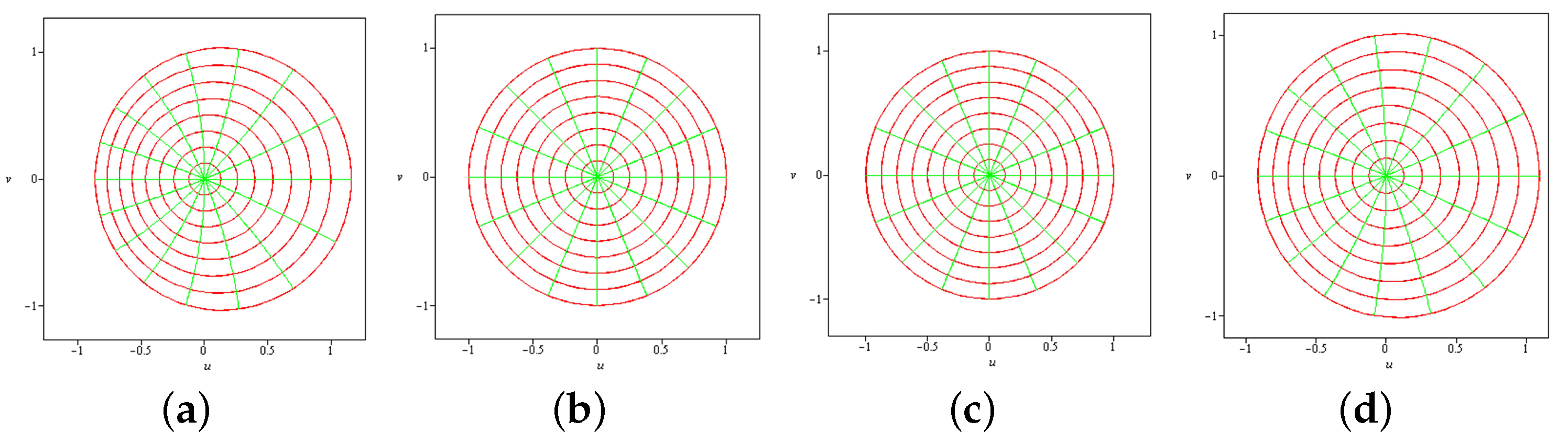
In
Figure 1, we provide the mappings of functions in
provided in Example 4.
Theorem 6. Let
- (a)
- (b)
If then
Proof. - (a)
It is a well-known result from [
28] that function
of the form (2) satisfies
and then
To prove that
consider
Then, we have to show that
By using the inequality
we may write
This proves the result.
- (b)
To show that
we consider the function
We prove that
Now,
This completes the result.
□
Corollary 1. Let
- (a)
Ifthen - (b)
If then
Corollary 2. Let
- (a)
- (b)
If then
Example 5. - (i)
- (ii)
- (iii)
- (iv)
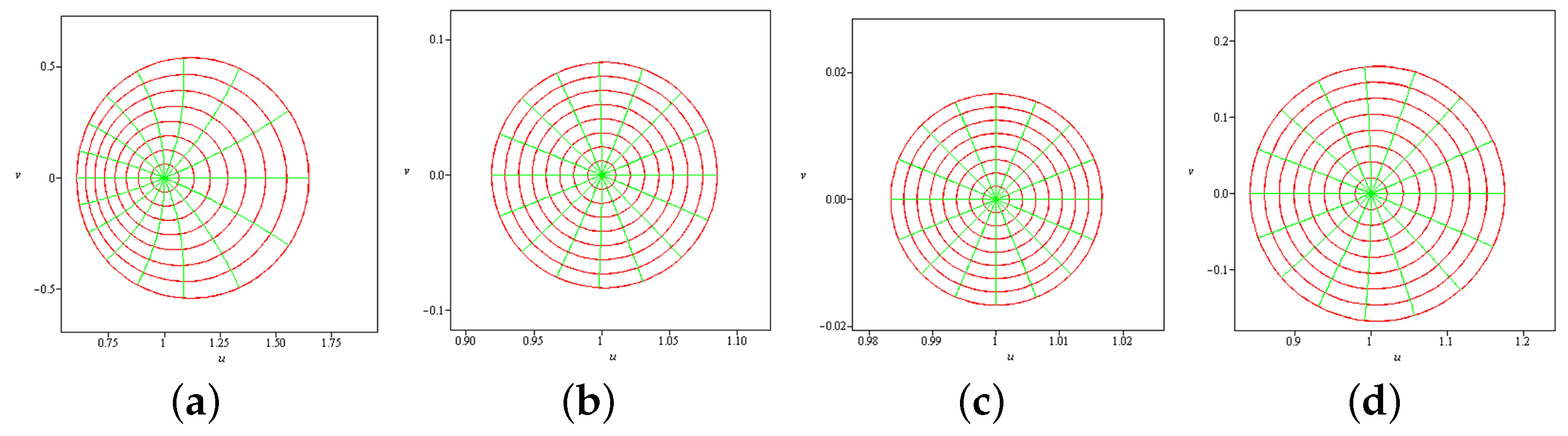
In
Figure 2, we provide the mappings of functions in
provided in Example 5.
Example 6. - (i)
- (ii)
- (iii)
- (iv)
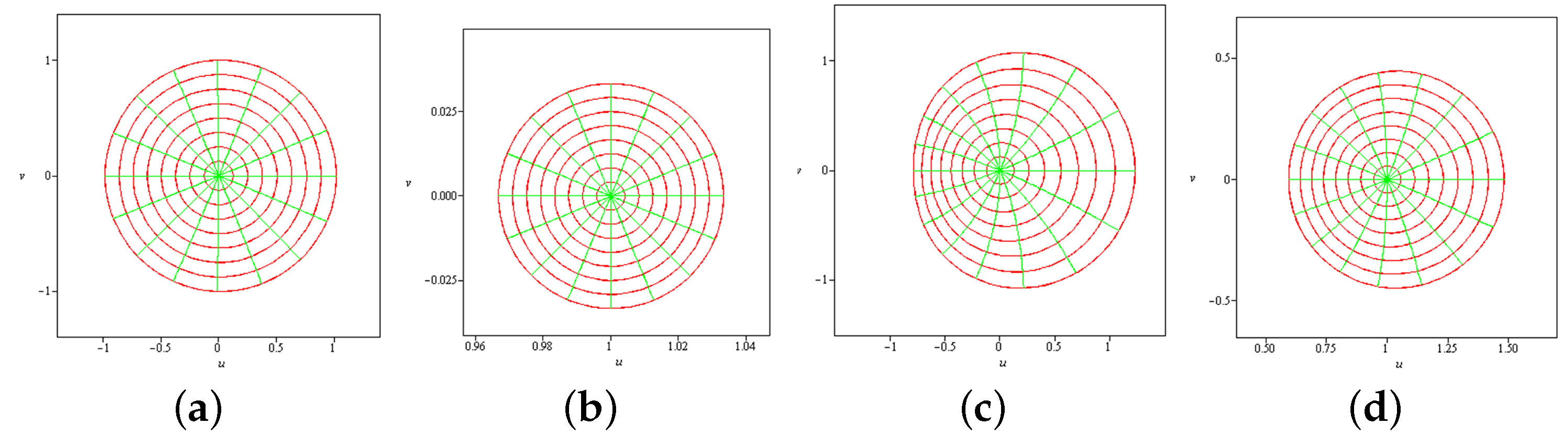
In
Figure 3, we provide the mappings of functions in
provided in Example 6.
4. Hardy Spaces of Rabotnov Functions
Hardy spaces of certain special functions have been studied by various authors. For instance, Ponnusay [
26] studied the problem for hypergeometric functions. The same problem by using the technique by Ponnusay for Bessel functions was used by Baricz [
15]. Hardy spaces of generalized Struve functions were studied by Yagmur and Orhan [
29]. The same problem for the case of Lommel functions was discussed by Yagmur [
30]. Hardy spaces of ML functions are discussed in [
9,
31].
Theorem 7. Let and Then,
- (i)
for
- (ii)
for
Proof. Since
therefore,
where
and
is any real number. Also, we have
Hence, cannot be written in the forms for and for , respectively By using Theorem 6 (a), therefore, an application of Lemma 7 leads to the required result. □
Theorem 8. Let and , and then ∈
Proof. It is given that
, which implies that
. Let
Now, using the definition of convolution
By applying Corollary 2 (b), it is evident that
Therefore, by using Lemma 5,
By using (3)
it follows that
for
and
for
This shows that
Moreover, we see that
Now, by using a result due to Macgregor [
32] (p. 533, Theorem 1) on the coefficients for the class
,
and the inequality
we may write
This shows that the series provided above absolutely converges in
for the given condition. Also, by using [
16] (p. 42, Theorem 3.11), the result
implies the continuity of
h on closure of
. Therefore,
h is bounded. This completes the result. □
Theorem 9. Let and . If , and then where
Proof. It is given that
which implies that
Let
. Then, it easy to see that
Now, by using Theorem 6 we have By using Lemma 6 and the given condition we have where . Hence, . □
Corollary 3. Let If then
Corollary 4. Let If then
Example 7. We see that the functionis in . We see that (see Figure 4a). Also, for by using Theorem 8, . Now, take and, utilizing Theorem 8, consider Here, Figure 4b shows that Also, (Figure 4c) for . This implies that . Hence, . In
Figure 4, we provide the mappings of functions in
provided in Example 7.
Figure 4.
Mappings of functions over provided in Example 7. (a) Mapping of over ; (b) mapping of over ; (c) mapping of over .
Figure 4.
Mappings of functions over provided in Example 7. (a) Mapping of over ; (b) mapping of over ; (c) mapping of over .
Example 8. Now, take and, utilizing Theorem 8, consider Here, Figure 5a shows that Also, (Figure 5b) for . This implies that . Hence, . Example 9. We take and, utilizing Theorem 8, consider Here, Figure 5c shows that Also, (Figure 5d) for . This implies that . Hence, . In
Figure 5, we provide the mappings of the above-presented examples in
.
5. Conclusions
We have studied various geometric properties of normalized Rabotnov functions in . In particular, we have found conditions on parameters so that the function is uniformly convex, strongly starlike, and strongly convex. Furthermore, we have discussed the starlikeness and convexity of order We have also studied conditions so that the Rabotnov functions belong to the class of bounded analytic functions and Hardy spaces. Various consequences of these results are also presented by taking particular values of the parameters s and u. These examples are also illustrated by the figures. The results presented here provide a variety of particular examples.
By applying these techniques, similar kinds of results can be obtained for functions that can be represented by the Taylor series. Some other geometric properties such as close-to-convexity, prestarlikeness, and inclusions in some other subclasses of univalent functions can further be studied. Moreover, radii problems for various classes of analytic functions can be discussed.


 ,
, 
