1. Extended Branciari Quasi-b-Distance
In the process of the rapid development of fixed-point theory, many new spaces have been emerged with their applications and the study of the newly emerged spaces. Such developments have been an interesting topic among the mathematical research community. A very interesting notion of
b-metric space was introduced by Bakhtin [
1] (later used by Czerwik in [
2,
3]). Branciari [
4] developed the notion of Branciari distance space via substituting triangle inequality by quadrilateral inequality, while Kamran et al. [
5] introduced the notion of extended
b-metric space. Mlaiki et al. [
6] introduced the concept of controlled metric type space by using two controlled functions in triangle inequality, and thus extended the work of Kamran et al. [
5].
Definition 1 ([
6])
. Let be a set and . A function is said to be a controlled metric type if, for all :- (dc1)
if and only if ,
- (dc2)
,
- (dc3)
.
The pair is called a controlled metric-type space.
Recently, Abdeljawad et al. [
7] have defined the notion of extended Branciari
b-metric space by combining extended
b-metric and Branciari distances.
Definition 2 ([
7])
. Let be a set and . A function is said to be an extended Branciari b-metric (-metric, for short) if it satisfies, for all , :- (ebb1)
if and only if ,
- (ebb2)
,
- (ebb3)
.
The pair will be called an extended Branciari b-metric space (EBbMS for short). If , then will be called a Branciari b-metric space.
In [
8], Zubair et al. combined the work of Mlaiki et al. [
6] and Abdeljawad et al. [
7], and introduced the controlled
b-Branciari metric-type space as follows:
Definition 3 ([
8])
. Let be a set and . A function is said to be a controlled b-Branciari metric type if it satisfies, for all distinct :- (dcb1)
if and only if ,
- (dcb2)
,
- (dcb3)
.
The pair is called a controlled b-Branciari metric-type space.
On the other hand, the notion of
b-metric space was generalized to quasi-b-metric space in [
9], and the concepts of right and left quasi-
b-metric spaces were established in [
10]. Jain et al. [
11] recently introduced the idea of extended Branciari quasi-
b-metric spaces and right and left completeness in these spaces, which represent an extension of the quasi-
b-metric spaces notion.
Definition 4. Let be a set and . A function is called an extended Branciari quasi-b-metric, if for all , and all distinct :
- (qeb1)
,
- (qeb2)
.
The triplet is then called an extended Branciari quasi-b-metric space (EBQbMS for short) with the coefficient .
Inspired by the above discussion, in the following sections, we are going to introduce the controlled extended Branciari quasi-b-metric spaces and its related notions.
Definition 5. Let be a set and . A function is said to be a controlled extended Branciari quasi-b-metric if it satisfies the following:
- (q1)
,
- (q2)
for all distinct . The pair is called a controlled extended Branciari quasi-b-metric space (controlled EBQbMS for short).
Definition 6. Let be a controlled EBQbMS and let be a sequence in ϝ and . The sequence converges to ϖ if and only if .
Remark 1. In a controlled EBQbMS, the uniqueness of limit is for a convergent sequence.
Definition 7. Let be a controlled EBQbMS and let be a sequence in ϝ. The sequence is said to be as follows:
- (i)
left--Cauchy if for every , there exists such that for all ,
- (ii)
right--Cauchy if for every , there exists such that for all ,
- (iii)
-Cauchy if for every , there exists such that for all .
Definition 8. Let be a controlled EBQbMS. Then is called the following:
- (i)
left--complete if every left--Cauchy sequence in ϝ is convergent,
- (ii)
right--complete if every right--Cauchy sequence in ϝ is convergent,
- (iii)
-complete if every -Cauchy sequence in ϝ is convergent.
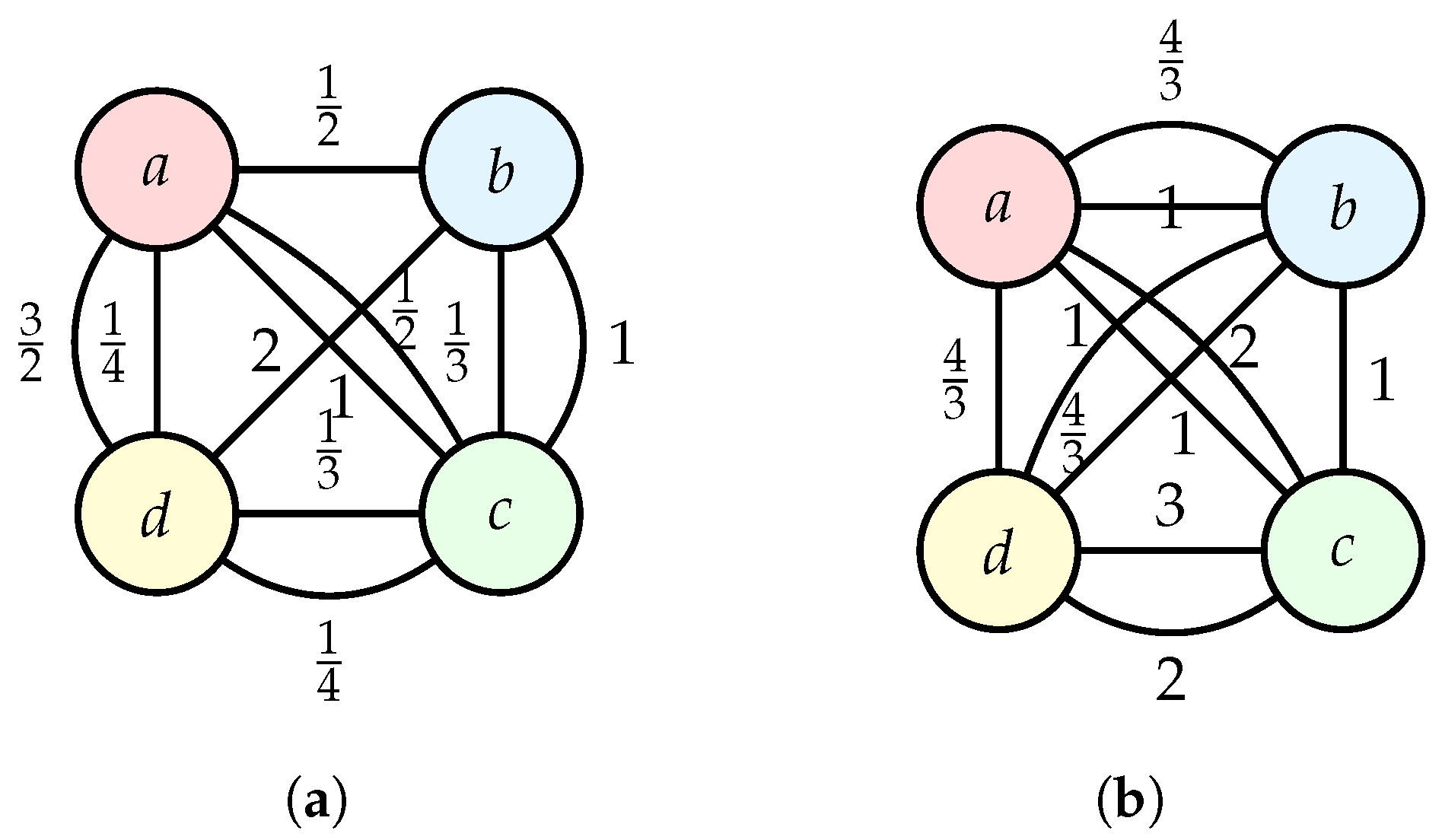
Definition 9. Let be a controlled EBQbMS. The mapping is continuous if each sequence for in ϝ is convergent to and the sequence converges to , that is, Example 1. Let be four cities of India, and suppose that there is only a one-way inter-city connection. Then, we define a set of nodes as . Denote as the fare between the cities, which is defined asNext, we denote the inter-city distances as and defineIn Figure 1, is demonstrated. It can be readily ascertained that is a controlled EBQbMS but not an EBQbMS as Example 2. Let . Define by Define asIn Figure 2, and θ are demonstrated. It can be readily ascertained that is a controlled EBQbMS asbut not an EBQbMS as The importance of this work lies in the fact that, in the context of right completeness (or left completeness), a new implicit relation makes it easier to demonstrate fixed-point results in a controlled EBQbMS space. In the context of underlining space, we also present novel ideas such as right and left Ulam–Hyers stability, right and left weak well-posed properties, right and left weak-limit shadowing properties, as well as their associated results. The two graphics depict a novel application to nonlinear matrix equations when using two illustrations. This demonstrates that our matrix equation solution assurance criteria are “weaker" than those previously derived in the literature. In addition, we used these findings to solve the fractional differential Riesz–Caputo equations with integral antiperiodic boundary values in the underlying space, and this was followed by an example demonstrating the validity of the result.
2. -Implicit Relations
The following notion was inspired by [
12]. Let
be a nonempty set. As denoted by
, the set of all functions
satisfy the following conditions:
- (i)
is increasing and ;
- (ii)
there exists such that
, for all , and , where denotes the n-th iterate of .
It is clear that and the class .
Example 3. Let be a controlled EBQbMS, where and . Consider the mapping , where . Note that . Thus,Therefore, and hence . We start by introducing a modified implicit relation, as in [
13,
14].
Let be the set of all functions satisfying the following conditions:
- (Ω1)
for all and , implies that there exists such that ;
- (Ω2)
If , then .
Example 4. Let , and .
- (Ω1)
Let , and .
Now, if , then we obtain , which gives as and , i.e., a contradiction. Therefore, we obtain , where so that .
- (Ω2)
If , that is, , then gives , which is a contradiction. Therefore, .
Example 5. Let , , and .
- (Ω1)
Let , and .
Then, . Hence, , where , . It is easy to check that , with , and can be chosen so that .
- (Ω2)
If , then it is a contradiction as . Therefore, .
3. Main Results
We introduced -implicit type mappings on a controlled EBbQMS.
Definition 10. Let be a controlled EBQbMS and . We then say that ℑ is a -implicit type mapping if there exists such that for , For a self-mapping ℑ on a set , it is denoted as .
Theorem 1. Let be a right--complete controlled EBQbMS with , and let be a continuous -implicit-type mapping where . Then, is a singleton set.
Proof. Let
and define a sequence
by
for all
. If
for some
, and we then come to the conclusion. Thus, assume that
for all
. Using (
1) with
and
, we have
that is,
Using
, we obtain that there is a
such that
and so
With the successive use of (
1) with
, we have
Similarly, if we take
and
, then we obtain
Next, we prove is a right--Cauchy sequence, that is, . We then discuss the two possible cases.
Case I. Let
,
. Then, by (q2), we have
that is,
.
Case II. Let
,
. Then, by (q2), we have
that is,
. Thus, by combining both cases,
for all
; hence, the sequence
is a right-
-Cauchy one.
Using the right-
-completeness of
, we can deduce that there exists
such that
as
, that is,
Using (q2), we have
Since
ℑ is continuous, by taking
, we obtain
, that is,
.
At last, we can show that
is a set of one. Assume, however, that there are different
. Through using (
1), we have
i.e.,
It follows from
that
, which implies that
. □
Example 6. Let and be as in Example 1, and let us denote ℑ on ϝ as the toll tax of the city and defineOnly Condition (1) of Theorem 1 has to be checked. When using Example 4, we have to checkfor and , where . Consider the following cases:
Case() If and (or and ; and ; or and ), then (5) holds trivially.
Case() Let and . Then,andso (5) reduces to . Case() Let and . Then,andso (5) reduces to . Case() Let and . Then,andso (5) reduces to . Case() Let and . Then,andso (5) reduces to . Case() Let and . Then, we haveandso (5) reduces to . Case() Let and . Then,andso (5) reduces to . Case() Let and . Then,andso (5) reduces to . Case() Let and . Then,andso (5) reduces to . If we take and , then in all the cases the contractive Condition (5) holds true. Hence, ℑ is a -implicit type mapping.
Thus, all the conditions of Theorem 1 are fulfilled and is the unique fixed point of ℑ.
By choosing from Examples 4 and 5, we obtain the following consequences.
Corollary 1. Let all the conditions of Theorem 1 be satisfied, except that the -implicit type condition is replaced by condition of the form (for all , with ). Thus, we have the following:
- (I)
where and , or - (II)
where and
Then, is a singleton.
6. Right and Left Weak Well-Posed Properties (Right and Left Weak Limit Shadowing)
The concept of a well posited fixed-point problem (FPP) has captured the attention of numerous mathematicians, including Popa [
19,
20] and others. The authors of the paper [
21] defined a weak well posed (wwp) property in a BbDS. In the following section, we will extend this concept to a controlled EBQbMS.
Definition 13. Let be a controlled EBQbMS, and let . The FPP of ℑ is said to be right [resp. left-] if it satisfies the following:
- 1.
;
- 2.
for any sequence in ϝ with and
, one has
[resp. for any sequence in ϝ with and
, one has ].
Theorem 5. Let be a right -complete controlled EBQbMS with , and let be continuous and satisfy Condition (9). Then, the FPP of ℑ is right wwp. Proof. Let
be a (unique) fixed point of
ℑ, and let
be a sequence in
such that
and
, for
. Owing to (q2), we have
By letting
in the above inequality, we obtain
WLOG. It is reasonable to presume that a subsequence of having distinct elements exists. Alternatively, there exists and such that for . As , . If , then since there is only one fixed point of ℑ. For , we obtain .
Using (
9) for
, we obtain
By letting
and using
, we have
which is not true. Thus, there exists
such that
. Then,
Therefore, from (
12), we have
Again, by using (
9), we obtain
i.e.,
By letting
and using the continuity of
ℑ, we obtain
which implies that
Therefore, from (
13), we obtain
which is a contradiction. Therefore,
. □
Theorem 6. Let be a left -complete controlled EBQbMS with , and let be continuous and satisfy Condition (9). Then, the FPP of ℑ is left wwp. There are some pieces of literature on the limit shadowing property of fpps ([
22,
23]). In order to investigate the right and left weak limit shadowing property (right wlsp/left wlsp) in a controlled EBQbMS, we first need to define these terms.
Definition 14. Let be a controlled EBQbMS and .
- 1.
The fpp of ℑ is said to have right wlsp in ϝ if assuming that in ϝ satisfies as and as . Thus, it follows that there exists such that as .
- 2.
The fpp of ℑ is said to have left wlsp in ϝ if assuming that in ϝ satisfies as and as . Thus, it follows that there exists such that as .
Theorem 7. Let be a right -complete controlled EBQbMS, and let be continuous and satisfy Condition (9) Then, ℑ has the right wlsp. Proof. Let , and let in be such that and . Since , , then, owing to Theorem 5, . Therefore, we obtain . □
Theorem 8. Let be a left -complete controlled EBQbMS, and let be continuous and satisfy (9). Then, ℑ has the left wlsp. 7. Applications to Riesz–Caputo Fractional Derivatives
In comparison to integer-order models, fractional-order models provide a more plausible account of memory and genetic processes. Riemann–Liouville and Riesz derivatives have been frequently used in the research on fractional boundary/initial value problems (FBVP/FIVP) in recent years. These fractional operators, however, are one-sided and can only alter the past or the future. The Riesz space fractional operator, in contrast to the other fractional operators, is a two-sided operator that captures both past and present non-local memory effects. This is critical because present states in the mathematical models of physical processes on finite domains are affected by both past and future memory effects. In the anomalous diffusion problem, for example, the Riesz fractional derivative has been utilized to account for memory effects in both past and future concentrations. The authors of [
24,
25,
26] addressed the solution of Riesz–Caputo fractional type BVP.
In this section, we investigate the uniqueness of a solution for an integral-type anti-periodic boundary value problem (APBVP) that is of a Riesz–Caputo fractional type of the form
where
is the Riesz–Caputo derivative,
is a continuous function, and
(where
X is a Banach space).
Before a discussion on the solutions of APBVP, we introduce the related notions.
Definition 15 ([
27])
. Let . The left and right Riemann–Liouville fractional integral of a function of order ζ is defined as follows: Definition 16. Let . The Riesz fractional integral of a function of order ζ is defined as follows: Definition 17 ([
27])
. Let , . Then, the left and right Caputo fractional derivatives of a function of order ζ are defined as follows:where is the ordinary differential operator. Definition 18. Let , . Then, the Riesz–Caputo fractional derivative of order ζ of a function is defined by Lemma 1 ([
27])
. Let and . Then, the following relations hold: When
and
, we have
Lemma 2. Suppose that and . Then, the fractional APBVP of order ζ in iswhich is equivalent to the integral equation of the form Proof. Owing to (
17) and (
18), we conclude that
Then,
By applying APBVP (
19), we have
When we insert the quantities that we have obtained for
and
into (
21), we obtain (
20). □
We are now able to bring up, with the appropriate conditions for our APBVP, a unique solution. Let be the space of continuous functions , which are defined on with the norm .
Theorem 9. Let be a continuous function. Assume that there exist non-negative real numbers , , such that for all , we have the following:
Then, Problem (14) has a unique solution on . Proof. We converted the fractional AVBVP (
14) and (
15) into a integral equation using the operator
of the form
For
and for each
, we have
Let
be defined by
Then,
is a complete controlled EBQbMS with the coefficient
. Then,
where
By virtue of Example 5,
ℑ is a
-implicit type mapping for
,
. Hence, following Theorem 1,
ℑ has a unique fixed point, that is, a solution to Equation (
14) with (
15). □
Remark 2. Lemma 2 and Theorem 9 generalize the work that is discussed in Wang and Wang [28]. Also, we used the generalized Banach fixed-point theorem 1 in a controlled EBQbMS to prove these results. Example 7. Consider the following nonlinear FDE with a Riesz–Caputo derivative:Here, , , , , and Therefore, (A1) and (A2) are satisfied with , and . Further,Thus, by Theorem 9, Problem (23) has a unique solution on . Example 8. Consider the following nonlinear FDE with a Riesz–Caputo derivative:Here, , , , , and Therefore, (A1) and (A2) are satisfied with , and . Further,Thus, by Theorem 9, Problem (24) has a unique solution on . 


