Article

Numerical Investigation of the Fractional Diffusion Wave Equation with the Mittag–Leffler Function

by
Madiha Shafiq
1,
Muhammad Abbas
1,*,
Emad K. El-Shewy
2,3,
Mahmoud A. E. Abdelrahman
4,5,
Noura F. Abdo
4,5 and
Ali A. El-Rahman
6,7
1
Department of Mathematics, University of Sargodha, Sargodha 40100, Pakistan
2
Department of Physics, College of Science, Taibah University, Al-Madinah Al-Munawarah 41411, Saudi Arabia
3
Theoretical Physics Group, Faculty of Science, Mansoura University, Mansoura 35516, Egypt
4
Department of Mathematics, College of Science, Taibah University, Al-Madinah Al-Munawarah 41411, Saudi Arabia
5
Department of Mathematics, Faculty of Science, Mansoura University, Mansoura 35516, Egypt
6
Department of Physics, College of Science and Humanities in Al-Kharj, Prince Sattam bin Abdulaziz University, Al-Kharj 11942, Saudi Arabia
7
Department of Physics, Faculty of Science, The New Valley University, Kharga Oasis 72714, Egypt
*
Author to whom correspondence should be addressed.
Fractal Fract. 2024, 8(1), 18; https://doi.org/10.3390/fractalfract8010018
Submission received: 23 September 2023 / Revised: 14 December 2023 / Accepted: 15 December 2023 / Published: 26 December 2023
(This article belongs to the Section Numerical and Computational Methods)

Abstract

:
A spline is a sufficiently smooth piecewise curve. B-spline functions are powerful tools for obtaining computational outcomes. They have also been utilized in computer graphics and computer-aided design due to their flexibility, smoothness and accuracy. In this paper, a numerical procedure dependent on the cubic B-spline (CuBS) for the time fractional diffusion wave equation (TFDWE) is proposed. The standard finite difference (FD) approach is utilized to discretize the Atangana–Baleanu fractional derivative (ABFD), while the derivatives in space are approximated through the CuBS with a θ -weighted technique. The stability of the propounded algorithm is analyzed and proved to be unconditionally stable. The convergence analysis is also studied, and it is of the order O ( h 2 + ( Δ t ) 2 ) . Numerical solutions attained by the CuBS scheme support the theoretical solutions. The B-spline technique gives us better results as compared to other numerical techniques.

1. Introduction

Fractional calculus (FC) is an area of mathematics that studies the integrals and derivatives of non-integer order as well as their applications. Leibniz [1] inquired about the derivative of order μ = 1 2 in a letter to L’Hôpital dated 30 September 1695. This day can be viewed as FC’s birthday. A comprehensive history of FC was discussed in [2,3]. However, it has attracted significant study interest in the last two decades due to its ability to solve a wide range of engineering and science problems: for example, bioengineering [4], heat and mass transfer [5], transport problems [6], damage and fatigue [7], groundwater flow problem [8,9], PID controllers [10], anomalous diffusion models [11], magnetic resonance imaging [12], hydrology cycle [13], economic processes [14] and coronavirus [15]. In many cases, fractional problems characterized by fractional partial differential equations (FPDEs) frequently behave more efficiently than their conventional integer-order counterparts. In general, it is impossible to acquire the exact solution of the maximum of FPDEs. As a consequence, finding numerical methods to analyze these models is becoming increasingly important.
In this paper, the following TFDWE with damping and reaction terms for different numerical outcomes shall be studied:
μ w ( q , t ) t μ + ψ w ( q , t ) t + ϑ w ( q , t ) 2 w ( q , t ) q 2 = p ( q , t ) , μ ( 1 , 2 ) , q [ a , b ] , t [ t 0 , T ] ,
with initial conditions (ICs):
w ( q , t 0 ) = α 1 ( q ) , w t ( q , t 0 ) = α 2 ( q )
and boundary conditions (BCs):
w ( a , t ) = β 1 ( t ) , w ( b , t ) = β 2 ( t ) ,
where ψ and ϑ are coefficients of the damping and reaction terms, respectively, p ( q , t ) is the source term, and w t ( q , t 0 ) represents the derivative of the function w ( q , t ) with respect to time t at t = t 0 . The ABFD μ t μ w ( q , t ) is described as:
μ t μ w ( q , t ) = R ( μ ) 2 μ 0 t 2 r 2 w ( q , r ) E μ μ 2 μ ( t r ) μ d r ,
where R ( μ ) is the normalization function and fulfills R ( 0 ) = R ( 1 ) = 1 . E μ , ς ( q ) is the Mittag–Leffler (ML) function satisfying E μ , 1 ( q ) = E μ ( q ) , which is given as:
E μ , ς ( q ) = z = 0 q z Γ ( μ z + ς ) .
Several papers have recently discussed the ABFD’s applicability. For example, Bas and Ozarslan [16] investigated population growth, logistics equations, Newton’s law of cooling and blood alcohol models with ABFD. Gómez-Aguilar et al. [17] employed the ABFD for electromagnetic waves. Ghanbari and Atangana [18] used ABFD in image processing. AIDS, Zika and macroeconomic models have been investigated by Gao et al. [19] with the help of ABFD. Ravichandran et al. [20] formulated a computer virus model involving ABFD. Hanif and Butt et al. [21] presented an optimal control method with ABFD for a dengue fever model. A coronavirus model using ABFD has been proposed by Goyal et al. [22].
In the literature, different methods have been put out to solve the TFDWE. Liu et al. [23] developed an FD discrete method for the TFDWE involving the Caputo fractional derivative (CFD). Huang et al. [24] constructed two FD schemes for the TFDWE. A meshless scheme for the TFDWE has been analyzed by Dehghan et al. [25]. For the TFDWE, Ali et al. [26] proposed a compact implicit difference algorithm. Wei [27] investigated the TFDWE using an FD/local discontinuous Galerkin scheme. Soltani Sarvestani et al. [28] established a wavelet method for a multi-term TFDWE with CFD. Huang et al. [29] developed efficient schemes for solving a non-linear TFDWE involving CFD. A pseudo-spectral scheme that depends on a reproducing kernel has been proposed by Fardi et al. [30]. Chen et al. [31] presented numerical and analytical solutions for a TFDWE with damping. A multistep method has been used by Yang et al. [32] for the computational solution to the TFDWE. Chen and Li [33] established an FD scheme for solving the TFDWE. A fictitious time integration algorithm has been constructed by Hashemi et al. [34] to solve the TFDWE with CFD.
B-spline functions have been employed by several researchers for solving FPDEs. Some work has been done by using these functions, and their detailed comparison with the proposed method is reported in Table 1. The novelty of the proposed work is to discretize the second-order time fractional derivative in the sense of the Atangana–Baleanu fractional operator μ ( 1 , 2 ) with a second-order implicit finite difference scheme, while in reference [35], the authors used the Atangana–Baleanu fractional operator μ ( 0 , 1 ) for discretization of the first-order time fractional derivative with a first-order implicit finite difference scheme, and in reference [36], the Caputo fractional derivative μ ( 0 , 1 ) with the Crank–Nicholson finite difference scheme has been used to discretize the first-order time fractional derivative. It can be easily seen that the work done in this paper is different from [35,36] because we have used a different problem with second-order fractional derivative discretization. This second-order time fractional derivative discretization in the sense of the Atangana–Baleanu fractional operator has never been used, as far as we are aware, for the case of the second-order TFDWE.
A cubic trigonometric B-spline (CTBS) collocation scheme for the TF diffusion equation (DE) has been propounded by Dhiman et al. [37]. Shafiq et al. [38] presented a numerical scheme for the TF Burgers’ equation (BE) involving ABFD. Majeed et al. [39] constructed an extended-CuBS-based technique for numerical simulation of the modified BE with CFD. For the linear TF Klein–Gordon equation (KGE), Khader and Abualnaja [40] proposed computational solutions by employing quadratic spline functions. A new CuBS scheme for numerical results for the Burgers’ and Fisher’s problems has been propounded by Majeed et al. [41]. Numerical simulations of the TFDE using a piecewise CuBS algorithm have been demonstrated by Shafiq et al. [42].
The propounded work is motivated by recent advances in the analysis of numerical simulations for the TFDWE. In this study, we designed and utilized a novel B-spline-based technique to solve the TFDWE. The current proposed method makes use of the second-order ABFD and the θ -weighted scheme. Implementation of the ABFD for the TFDWE is novel in B-spline techniques. In addition, examination of the scheme’s convergence and stability is carried out. To the greatest extent of the authors’ awareness, the offered TFDWE method is novel and has not previously been mentioned in the literature.
This paper is formatted as follows: In Section 2, the CuBS functions and Parseval’s identity (PI) are appended. The presented methodology is formulated in Section 3. The current method’s stability and convergence are included in Section 4 and Section 5, respectively. The efficacy and validity of the proposed technique are explored in Section 6, and finally, in Section 7, the research work is concluded.

2. Preliminaries

Definition 1.
If g ˜ L 2 [ a , b ] , then PI is defined as [43]:
n = | g ^ ( n ) | 2 = a b | g ˜ ( q ) | 2 d q ,
where g ^ ( n ) = a b g ˜ ( q ) e 2 π i n q d q is the Fourier transform for all integers n.

Basis Functions

Consider a = q 0 < q 1 < < q N = b to be the equivalent partition of [ a , b ] , where q s = q 0 + s h , s = 0 , 1 , , N , with h = b a N . The CuBS functions are expressed as [35]:
C s ( q ) = 1 6 h 3 ( q q s 2 ) 3 , if   q [ q s 2 , q s 1 ) , h 3 + 3 h 2 ( q q s 1 ) + 3 h ( q q s 1 ) 2 3 ( q q s 1 ) 3 , if   q [ q s 1 , q s ) , h 3 + 3 h 2 ( q s + 1 q ) + 3 h ( q s + 1 q ) 2 3 ( q s + 1 q ) 3 , if   q [ q s , q s + 1 ) , ( q s + 2 q ) 3 , if   q [ q s + 1 , q s + 2 ) , 0 , otherwise ,
where q is the variable. The CuBS has geometrical characteristics such as the partition of unity, non-negativity, the convex hull property, symmetry and geometric invariability [38]. In addition, C 1 , C 0 , , C N + 1 have been established. For w ( q , t ) , the estimation W ( q , t ) in terms of the CuBS can be presumed as [42]:
W ( q , t ) = s = 1 N + 1 φ s ( t ) C s ( q ) ,
where unknown points φ s ( t ) are to be computed at every temporal stage. Equations (7) and (8) provide the following approximations at the nodal points:
W ( q s , t ) = ( W ) s = 1 6 φ s 1 + 4 6 φ s + 1 6 φ s + 1 , W q ( q s , t ) = ( W q ) s = 1 2 h φ s 1 + 1 2 h φ s + 1 , W q q ( q s , t ) = ( W q q ) s = 1 h 2 φ s 1 + 2 h 2 φ s + 1 h 2 φ s + 1 .

3. Description of Numerical Scheme

The given problem’s time derivative is discretized using the ABFD. Suppose 0 = t 0 < t 1 < < t M = T is the equivalent partition of [ 0 , T ] , where t m = m Δ t , m = 0 , 1 , , M with Δ t = T M . Now we discretize the time derivative at t = t m + 1 as
μ t μ w ( q , t m + 1 ) = R ( μ ) 2 μ 0 t m + 1 2 r 2 w ( q , r ) E μ μ 2 μ ( t m + 1 r ) μ d r , 1 < μ < 2 , = R ( μ ) 2 μ y = 0 m t y t y + 1 2 r 2 w ( q , r ) E μ μ 2 μ ( t m + 1 r ) μ d r .
Using the forward difference approach, Equation (10) becomes
μ t μ w ( q , t m + 1 ) = R ( μ ) 2 μ y = 0 m w ( q , t y + 1 ) 2 w ( q , t y ) + w ( q , t y 1 ) ( Δ t ) 2 t y t y + 1 E μ μ 2 μ ( t m + 1 r ) μ d r + ϖ Δ t m + 1 , = R ( μ ) Δ t ( 2 μ ) y = 0 m w ( q , t m y + 1 ) 2 w ( q , t m y ) + w ( q , t m y 1 ) { ( y + 1 ) E μ , 2 μ 2 μ ( y + 1 ) Δ t μ y E μ , 2 μ 2 μ ( y Δ t ) μ } + ϖ Δ t m + 1 , = R ( μ ) Δ t ( 2 μ ) y = 0 m w ( q , t m y + 1 ) 2 w ( q , t m y ) + w ( q , t m y 1 ) ( y + 1 ) E y + 1 y E y + ϖ Δ t m + 1 .
Hence, Equation (11) gives
μ t μ w ( q , t m + 1 ) = R ( μ ) Δ t ( 2 μ ) y = 0 m v y w ( q , t m y + 1 ) 2 w ( q , t m y ) + w ( q , t m y 1 ) + ϖ Δ t m + 1 ,
where E y = E μ , 2 μ 2 μ ( y Δ t ) μ and v y = ( y + 1 ) E y + 1 y E y . Furthermore, the truncation error ϖ Δ t m + 1 is given by
| ϖ Δ t m + 1 | ( Δ t ) 2 ,
where ℧ is a constant. Employing a θ -weighted scheme and Equation (12), Equation (1) is transformed to
R ( μ ) Δ t ( 2 μ ) y = 0 m v y w ( q , t m y + 1 ) 2 w ( q , t m y ) + w ( q , t m y 1 ) + ψ Δ t w ( q , t m + 1 ) w ( q , t m ) + θ ϑ w ( q , t m + 1 ) w q q ( q , t m + 1 ) + ( 1 θ ) ϑ w ( q , t m ) w q q ( q , t m ) = p ( q , t m + 1 ) .
Discretizing (14) for θ = 1 , we achieve
( ξ E 1 + ψ 0 + ϑ ) w s m + 1 ( 2 ξ E 1 + ψ 0 ) w s m + ξ E 1 w s m 1 + ξ y = 1 m v y w s m y + 1 2 w s m y + w s m y 1 ( w q q ) s m + 1 = p s m + 1 , m = 0 , 1 , , M ,
where ξ = R ( μ ) Δ t ( 2 μ ) , ψ 0 = ψ Δ t , w s m = w ( q s , t m ) , and p s m + 1 = p ( q s , t m + 1 ) . It is detected that the term w 1 will appear when m = y or m = 0 . To make w 1 vanish, we employ the IC to attain
w 1 = w 1 2 Δ t α 2 ( q ) .
Using the CuBS approximation and its required derivatives at the knot q s in Equation (15), then
( ξ E 1 + ψ 0 + ϑ ) W s m + 1 ( W q q ) s m + 1 = ( 2 ξ E 1 + ψ 0 ) W s m ξ E 1 W s m 1 ξ y = 1 m v y [ W s m y + 1 2 W s m y + W s m y 1 ] + p s m + 1 .
Substituting (9) into (17), we get
1 6 ( ξ E 1 + ψ 0 + ϑ ) 1 h 2 φ s 1 m + 1 + 4 6 ( ξ E 1 + ψ 0 + ϑ ) + 2 h 2 φ s m + 1 + 1 6 ( ξ E 1 + ψ 0 + ϑ ) 1 h 2 φ s + 1 m + 1 = ( 2 ξ E 1 + ψ 0 ) 1 6 φ s 1 m + 4 6 φ s m + 1 6 φ s + 1 m ξ E 1 1 6 φ s 1 m 1 + 4 6 φ s m 1 + 1 6 φ s + 1 m 1 ξ y = 1 m v y [ 1 6 ( φ s 1 m y + 1 2 φ s 1 m y + φ s 1 m y 1 ) + 4 6 ( φ s m y + 1 2 φ s m y + φ s m y 1 ) + 1 6 ( φ s + 1 m y + 1 2 φ s + 1 m y + φ s + 1 m y 1 ) ] + p s m + 1 .
The system (18) has N + 1 linear equations with N + 3 unknowns. To get a consistent system, two more equations are acquired by employing the BCs (3). Hence, a matrix system of algebraic equations with ( N + 3 ) × ( N + 3 ) dimension is achieved; it can be uniquely solved using any suitable algorithm. Before utilizing (18), the initial vector φ 0 = [ φ 1 0 , φ 0 0 , , φ N + 1 0 ] T is attained through the ICs as
( W q ) s 0 = α 1 ( q s ) , s = 0 , ( W ) s 0 = α 1 ( q s ) , s = 0 , 1 , , N , ( W q ) s 0 = α 1 ( q s ) , s = N .
The matrix form of Equation (19) is represented as
F φ 0 = D ,
where
F = 1 2 h 0 1 2 h 1 6 4 6 1 6 1 6 4 6 1 6 1 6 4 6 1 6 1 6 4 6 1 6 1 2 h 0 1 2 h and D = α 1 ( q 0 ) α 1 ( q 0 ) α 1 ( q 1 ) α 1 ( q N 1 ) α 1 ( q N ) α 1 ( q N ) .
Any numerical algorithm can be used to solve Equation (20) for φ 0 . Mathematica 12 is utilized to accomplish the numerical results.

4. The Stability of the Presented Scheme

If the error does not increase while the algorithm is running, it can be deemed that the computational method is stable [44]. The Fourier technique is utilized to ensure the proposed scheme’s stability. For this, presume that ϵ ˜ s m and ϵ s m indicate the growth factors numerically and analytically, respectively. The error Φ s m can be written as
Φ s m = ϵ s m ϵ ˜ s m , s = 1 , , N 1 , m = 0 , 1 , M .
Thus, from Equation (18), we obtain
1 6 ( ξ E 1 + ψ 0 + ϑ ) 1 h 2 Φ s 1 m + 1 + 4 6 ( ξ E 1 + ψ 0 + ϑ ) + 2 h 2 Φ s m + 1 + 1 6 ( ξ E 1 + ψ 0 + ϑ ) 1 h 2 Φ s + 1 m + 1 = ( 2 ξ E 1 + ψ 0 ) 1 6 Φ s 1 m + 4 6 Φ s m + 1 6 Φ s + 1 m ξ E 1 1 6 Φ s 1 m 1 + 4 6 Φ s m 1 + 1 6 Φ s + 1 m 1 ξ y = 1 n v y [ 1 6 ( Φ s 1 m y + 1 2 Φ s 1 m y + Φ s 1 m y 1 ) + 4 6 ( Φ s m y + 1 2 Φ s m y + Φ s m y 1 ) + 1 6 ( Φ s + 1 m y + 1 2 Φ s + 1 m y + Φ s + 1 m y 1 ) ] .
Through ICs and BCs, we can write
Φ s 0 = α 1 ( q s ) , ( Φ t ) s 0 = α 2 ( q s ) , s = 1 , 2 , , N
and
Φ 0 m = β 1 ( t m ) , Φ N m = β 2 ( t m ) , m = 0 , 1 , , M .
The grid function is as follows:
Φ m = Φ s m , q q s h 2 , q s + h 2 , s = 1 , 2 , , N 1 , 0 , q a , a + h 2 or q b h 2 , b .
The Fourier mode of Φ m ( q ) can be presented as:
Φ m ( q ) = n = Ω m ( n ) e 2 π i n q b a ,
where
Ω m ( n ) = 1 b a a b Φ m ( q ) e 2 π i n q b a d q , m = 0 , 1 , , M and Φ m = [ Φ 1 m , Φ 2 m , , Φ N 1 m ] T .
Implementing the . 2 norm, we have
Φ m 2 = s = 1 N 1 h | Φ s m | 2 , = a a + h 2 | Φ m | 2 d q + s = 1 N 1 q s h 2 q s + h 2 | Φ m | 2 d q + b h 2 b | Φ m | 2 d q 1 2 , = a b | Φ m | 2 d q 1 2 .
Utilizing Parseval’s identity (6), we attain
a b | Φ m | 2 d q = n = | Ω m ( n ) | 2 .
Hence, we acquire
Φ m 2 2 = n = | Ω m ( n ) | 2 .
Assume that Equations (22)–(24) possess a solution in the Fourier mode as:
Φ s m = Ω m e i ϱ s h ,
where i = 1 , and ϱ is any real number. Inserting (29) into (22) and simplifying, we achieve
1 6 ( ξ E 1 + ψ 0 + ϑ ) 1 h 2 Ω m + 1 e i ϱ h + 4 6 ( ξ E 1 + ψ 0 + ϑ ) + 2 h 2 Ω m + 1 + 1 6 ( ξ E 1 + ψ 0 + ϑ ) 1 h 2 Ω m + 1 e i ϱ h = ( 2 ξ E 1 + ψ 0 ) 1 6 Ω m e i ϱ h + 4 6 Ω m + 1 6 Ω m e i ϱ h ξ E 1 6 Ω m 1 e i ϱ h + 4 ξ E 1 6 Ω m 1 + ξ E 1 6 Ω m 1 e i ϱ h y = 1 m v y [ ξ 6 Ω m y + 1 e i ϱ h 2 Ω m y e i ϱ h + Ω m y 1 e i ϱ h + 4 ξ 6 Ω m y + 1 2 Ω m y + Ω m y 1 + ξ 6 Ω m y + 1 e i ϱ h 2 Ω m y e i ϱ h + Ω m y 1 e i ϱ h ] .
Utilizing the relation e i ϱ h + e i ϱ h = 2 c o s ( ϱ h ) and simplifying, then Equation (30) gives
Ω m + 1 = ( 1 + γ ) σ Ω m γ σ Ω m 1 γ σ E 1 y = 1 m v y Ω m y + 1 2 Ω m y + Ω m y 1 ,
where γ = ξ E 1 ξ E 1 + ψ 0 and σ = 1 + 2 cos ( ϱ h ) ( ϑ h 2 6 ) + 4 ϑ h 2 + 12 ( ξ E 1 h 2 + ψ 0 h 2 ) ( 2 cos ( ϱ h ) + 4 ) . Obviously, E 1 > 0 and σ 1 .
Proposition 1.
If Ω m is the solution for Equation (31), then | Ω m | ( 1 + γ ) | Ω 0 | , m = 0 , 1 , , M .
Proof. 
To demonstrate this, mathematical induction is employed. For m = 0 , Equation (31) yields
| Ω 1 | = ( 1 + γ ) σ | Ω 0 | ( 1 + γ ) | Ω 0 | , σ 1 .
Assume that | Ω m | ( 1 + γ ) | Ω 0 | for m = 1 , 2 , , M 1 ; then,
| Ω m + 1 | ( 1 + γ ) σ | Ω m | γ σ | Ω m 1 | γ σ E 1 y = 1 m v y | Ω m y + 1 | 2 | Ω m y | + | Ω m y 1 | , ( 1 + γ ) 2 σ | Ω 0 | γ ( 1 + γ ) σ | Ω 0 | γ ( 1 + γ ) σ E 1 y = 1 m v y | Ω 0 | 2 | Ω 0 | + | Ω 0 | , = ( 1 + γ ) σ [ 1 + γ γ ] | Ω 0 | , | Ω m + 1 | ( 1 + γ ) | Ω 0 | .
 □
Theorem 1.
The proposed scheme (18) solving the TFDWE (1)–(3) is unconditionally stable.
Proof. 
Using expression (28) and Proposition 1, we achieve
Φ m 2 ( 1 + γ ) Φ 0 2 , 0 m M .
Consequently, the proposed computational technique is stable unconditionally. □

5. The Convergence of the Presented Scheme

The methodology described in [45] is utilized to examine the convergence of the proposed approach. First and foremost, the following theorem is stated as [46,47]:
Theorem 2.
Suppose the partition of [ a , b ] is ε = { a = q 0 , q 1 , , q N = b } with q s = a + s h , where s = 0 , 1 , , N ; also, p belongs to C 2 [ a , b ] and w ( q , t ) belongs to C 4 [ a , b ] . If solution curve w ( q , t ) is interpolated by unique spline W ˜ ( q , t ) at q s ε , then for every t 0 there exist positive constants χ s independent of h; for s = 0 , 1 , 2 , we have
D s w ( q , t ) W ˜ ( q , t ) χ s h 4 s .
Lemma 1.
The CuBS set { C s ( q ) } s = 1 N + 1 in (7) fulfills the following inequality as provided in [42]:
s = 1 N + 1 | C s ( q ) | 5 3 , a q b .
Theorem 3.
If p is a member of C 2 [ 0 , 1 ] , and, furthermore, the computational solution W ( q , t ) to the analytical solution w ( q , t ) for TFDWE (1)–(3) exists, then
w ( q , t ) W ( q , t ) χ ˜ h 2 , t 0 ,
when h is small enough and χ ˜ > 0 is independent of h.
Proof. 
Let W ˜ ( q , t ) = s = 1 N + 1 l s m ( t ) C s ( q ) be the unique CuBS interpolant for W ( q , t ) . The triangular inequality yields
w ( q , t ) W ( q , t ) w ( q , t ) W ˜ ( q , t ) + W ˜ ( q , t ) W ( q , t ) .
Using inequality (32) for s = 0 in Equation (35), we get
w ( q , t ) W ( q , t ) χ 0 h 4 + W ˜ ( q , t ) W ( q , t ) .
The current approach has collocation conditions p ( q s , t ) = L W ( q s , t ) = L w ( q s , t ) , s = 0 , 1 , , N . Consider
L W ˜ ( q s , t ) = p ˜ ( q s , t ) .
Consequently, L ( W ˜ ( q s , t ) W ( q s , t ) ) is written at t = t m as
1 6 ( ξ E 1 + ψ 0 + ϑ ) 1 h 2 s 1 m + 1 + 4 6 ( ξ E 1 + ψ 0 + ϑ ) + 2 h 2 s m + 1 + 1 6 ( ξ E 1 + ψ 0 + ϑ ) 1 h 2 s + 1 m + 1 = ( 2 ξ E 1 + ψ 0 ) 1 6 s 1 m + 4 6 s m + 1 6 s + 1 m ξ E 1 1 6 s 1 m 1 + 4 6 s m 1 + 1 6 s + 1 m 1 ξ y = 1 m v y [ 1 6 ( s 1 m y + 1 2 s 1 m y + s 1 m y 1 ) + 4 6 ( s m y + 1 2 s m y + s m y 1 ) + 1 6 ( s + 1 m y + 1 2 s + 1 m y + s + 1 m y 1 ) ] + 1 h 2 s m + 1 .
The BCs can be provided as
1 6 s 1 m + 1 + 4 6 s m + 1 + 1 6 s + 1 m + 1 = 0 , s = 0 , N ,
where
s m = φ s m l s m , s = 1 , 0 , , N + 1
and
s m = h 2 [ p s m p ˜ s m ] , s = 0 , 1 , , N .
Through inequality (32), we attain
| s m | = h 2 | p s m p ˜ s m | χ h 4 .
Define m = max 0 s N | s m | , e s m = | s m | and e m = max 0 s N | e s m | . When m = 0 and by utilizing expression (16), Equation (37) yields
1 6 ( ψ 0 + ϑ ) 1 h 2 s 1 1 + 4 6 ( ψ 0 + ϑ ) + 2 h 2 s 1 + 1 6 ( ψ 0 + ϑ ) 1 h 2 s + 1 1 = ψ 0 1 6 s 1 0 + 4 6 s 0 + 1 6 s + 1 0 + 1 h 2 s 1 ,
where s = 0 , 1 , , N . Employing IC, e 0 = 0 :
4 6 ( ψ 0 + ϑ ) + 2 h 2 s 1 = 1 6 ( ψ 0 + ϑ ) 1 h 2 ( s 1 1 + s + 1 1 ) + 1 h 2 s 1 .
Taking absolute values of s 1 and s 1 and for an adequately small h, we get
e s 1 3 χ h 4 h 2 ( ψ 0 + ϑ ) + 12 , 0 s N .
We get the values e 1 1 and e N + 1 1 through BCs:
e 1 1 15 χ h 4 h 2 ( ψ 0 + ϑ ) + 12 ,
e N + 1 1 15 χ h 4 h 2 ( ψ 0 + ϑ ) + 12 ,
which implies
e 1 χ 1 h 2 ,
where χ 1 does not depend on h.
Now, mathematical induction is utilized for the proof of this theorem. Suppose that e s x χ x h 2 is true for 1 x n and χ = m a x { χ x : x = 0 , 1 , , n } ; then from Equation (37), we get
1 6 ( ξ E 1 + ψ 0 + ϑ ) 1 h 2 s 1 m + 1 + 4 6 ( ξ E 1 + ψ 0 + ϑ ) + 2 h 2 s m + 1 + 1 6 ( ξ E 1 + ψ 0 + ϑ ) 1 h 2 s + 1 m + 1 = ( 2 ξ E 1 + ψ 0 ξ v 1 ) 1 6 s 1 m + 4 6 s m + 1 6 s + 1 m ξ [ ( v 0 2 v 1 + v 2 ) 1 6 s 1 m 1 + 4 6 s m 1 + 1 6 s + 1 m 1 + ( v 1 2 v 2 + v 3 ) 1 6 s 1 m 2 + 4 6 s m 2 + 1 6 s + 1 m 2 + ( v 2 2 v 3 + v 4 ) 1 6 s 1 m 3 + 4 6 s m 3 + 1 6 s + 1 m 3 + + ( v m 3 2 v m 2 + v m 1 ) 1 6 s 1 2 + 4 6 s 2 + 1 6 s + 1 2 + ( v m 2 2 v m 1 + v m ) ( 1 6 s 1 1 + 4 6 s 1 + 1 6 s + 1 1 ) + v m 1 1 6 s 1 0 + 4 6 s 0 + 1 6 s + 1 0 v m 1 6 s 1 1 + 4 6 s 1 + 1 6 s + 1 1 ] + 1 h 2 s m + 1 .
Again, taking absolute values of s m + 1 and s m + 1 , we achieve
e s m + 1 3 h 2 h 2 ( ξ E 1 + ψ 0 + ϑ ) + 12 ( 2 ξ E 1 + ψ 0 ξ v 1 ) χ h 2 ξ y = 1 m 1 ( v y 1 2 v y + v y + 1 ) χ h 2 + ξ v m χ h 2 + χ h 2 .
Like before, we obtain the values of e 1 m + 1 and e N + 1 m + 1 from the BCs:
e 1 m + 1 15 h 2 h 2 ( ξ E 1 + ψ 0 + ϑ ) + 12 ( 2 ξ E 1 + ψ 0 ξ v 1 ) χ h 2 ξ y = 1 m 1 ( v y 1 2 v y + v y + 1 ) χ h 2 + ξ v m χ h 2 + χ h 2
and
e N + 1 m + 1 15 h 2 h 2 ( ξ E 1 + ψ 0 + ϑ ) + 12 ( 2 ξ E 1 + ψ 0 ξ v 1 ) χ h 2 ξ y = 1 m 1 ( v y 1 2 v y + v y + 1 ) χ h 2 + ξ v m χ h 2 + χ h 2 .
Consequently, for all m, we get
e m + 1 χ h 2 .
In particular,
W ˜ ( q , t ) W ( q , t ) = s = 1 N + 1 l s ( t ) φ s ( t ) C s ( q ) .
Thus, from Lemma 1 and inequality (38), we attain
W ˜ ( q , t ) W ( q , t ) 5 3 χ h 2 .
Using (39), the inequality (36) yields
w ( q , t ) W ( q , t ) χ 0 h 4 + 5 3 χ h 2 = χ ˜ h 2 ,
where χ ˜ = χ 0 h 2 + 5 3 χ . □
Theorem 4.
The numerical scheme (18) for TFDWE is convergent with respect to ICs and BCs.
Proof. 
Assume that W ( q , t ) and w ( q , t ) are approximate and analytical solutions, respectively, for the TFDWE. Thus, the preceding theorem and relation (13) support the existence of constants χ ˜ and ℧ such that
w ( q , t ) W ( q , t ) χ ˜ h 2 + ( Δ t ) 2 .
Therefore, the proposed approach is second-order convergent. □

6. Numerical Results and Discussion

In this section, numerical results of some experiments utilizing the proposed approach are demonstrated. To investigate the efficacy of the proposed technique, we utilize error norms L and L 2 as
L = w ( q s , t ) W ( q s , t ) = max 0 s N | w ( q s , t ) W ( q s , t ) |
and
L 2 = w ( q s , t ) W ( q s , t ) 2 = h s = 0 N | w ( q s , t ) W ( q s , t ) | 2 .
In addition, the convergence order is measured as
log 2 L ( N ) L ( 2 N ) .
All of the examples are investigated by taking R ( μ ) = 1 . Numerical calculations are carried out by utilizing Mathematica 12 on an Intel(R) Core(TM) i5-3437U CPU @ 1.90 GHz (2.40 GHz Turbo), 12.0 GB RAM, an SSD and a 64-bit operating system (Windows 10).
Example 1.
Consider the TFDWE
μ w ( q , t ) t μ 2 w ( q , t ) q 2 = p ( q , t ) , μ ( 1 , 2 ) , t [ 0 , 1 ] , q [ 0 , 1 ] ,
with ICs
w ( q , 0 ) = 0 , w t ( q , 0 ) = sin ( π q )
and BCs
w ( 0 , t ) = w ( 1 , t ) = 0 ,
where p ( q , t ) = 2 R ( μ ) 2 μ t sin ( π q ) E μ , 2 μ 2 μ t μ + π 2 ( t 2 t ) sin ( π q ) .
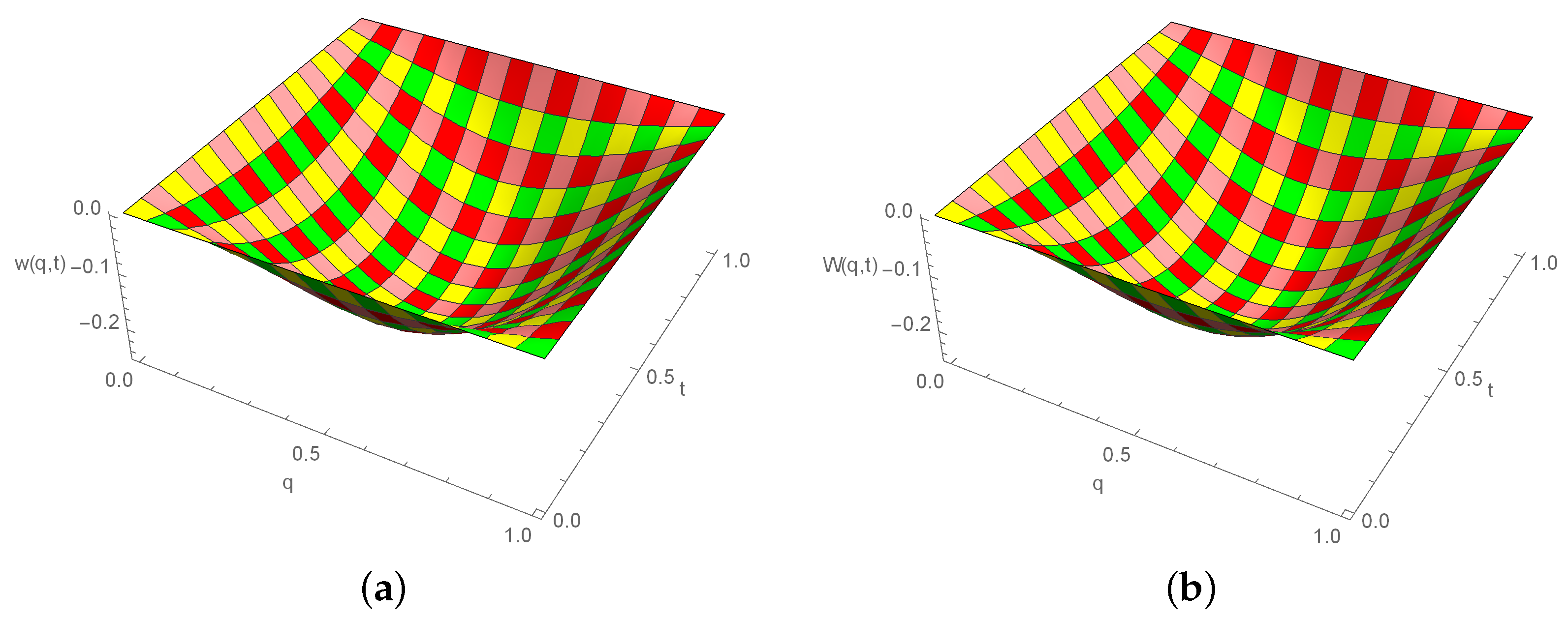
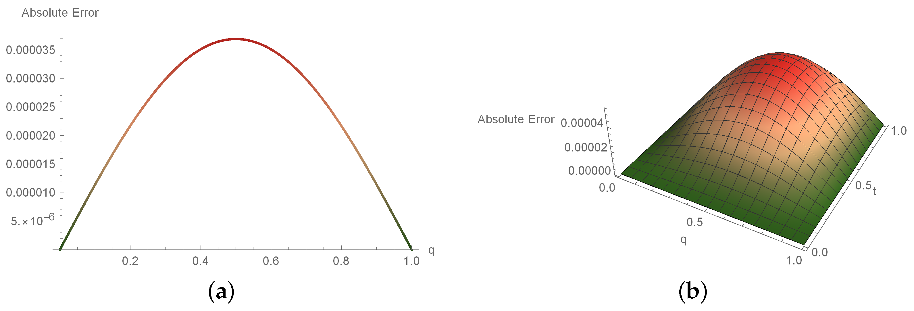
The expression w ( q , t ) = ( t 2 t ) sin ( π q ) is the exact solution. For Example 1, the absolute errors for distinct q values at t = 0.2 are displayed in Table 2. For various temporal stages, error norms L and L 2 are demonstrated in Table 3. Table 4 comprises the analysis of the convergence order and error norms. Table 5, Table 6 and Table 7 describe the error norms at several values of Δ t and h. Figure 1 reveals the relation between numerical outcomes and analytical solutions at different temporal directions. A 3D plot of the analytical and approximate solutions is demonstrated in Figure 2. Figure 3 expounds on the descriptions of the 2D and 3D errors.
Example 2.
Consider the TFDWE
μ w ( q , t ) t μ + w ( q , t ) t 2 w ( q , t ) q 2 = p ( q , t ) , μ ( 1 , 2 ) , t [ 0 , 1 ] , q [ 0 , 1 ] ,
with ICs
w ( q , 0 ) = 0 , w t ( q , 0 ) = 0
and BCs
w ( 0 , t ) = w ( 1 , t ) = 0 ,
where p ( q , t ) = 2 R ( μ ) 2 μ t q ( 1 q ) E μ , 2 μ 2 μ t μ + 2 t q ( 1 q ) + 2 t 2 .
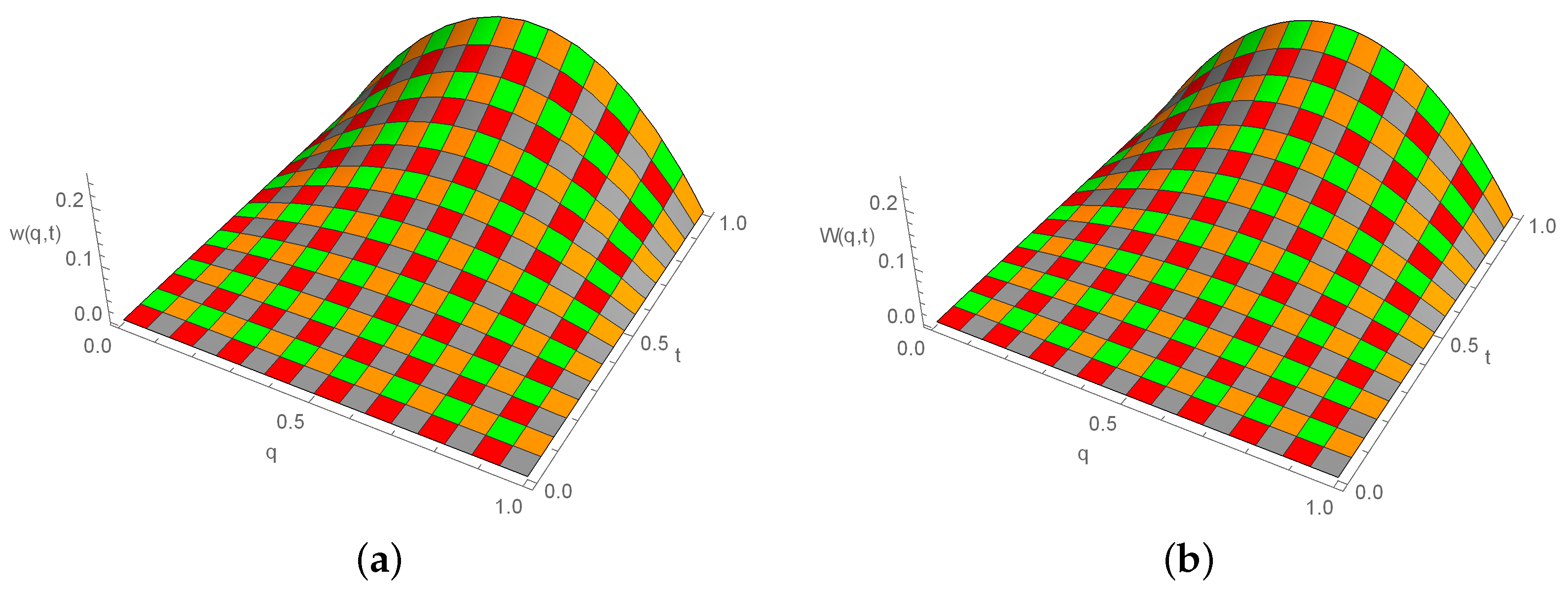
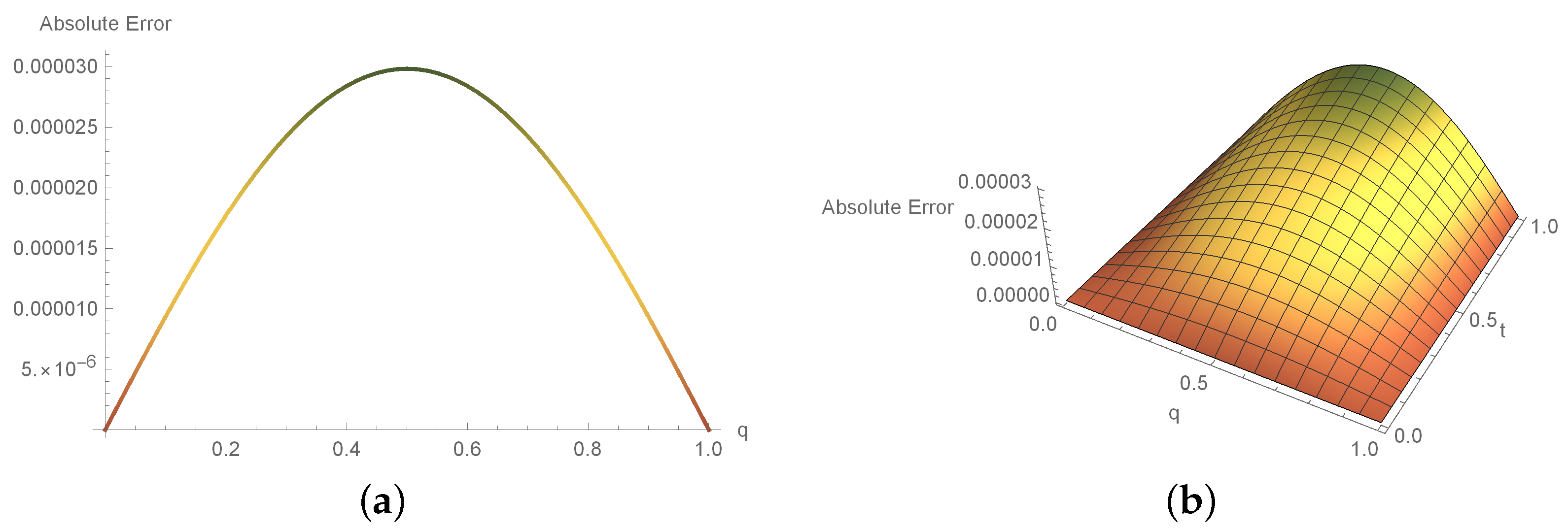
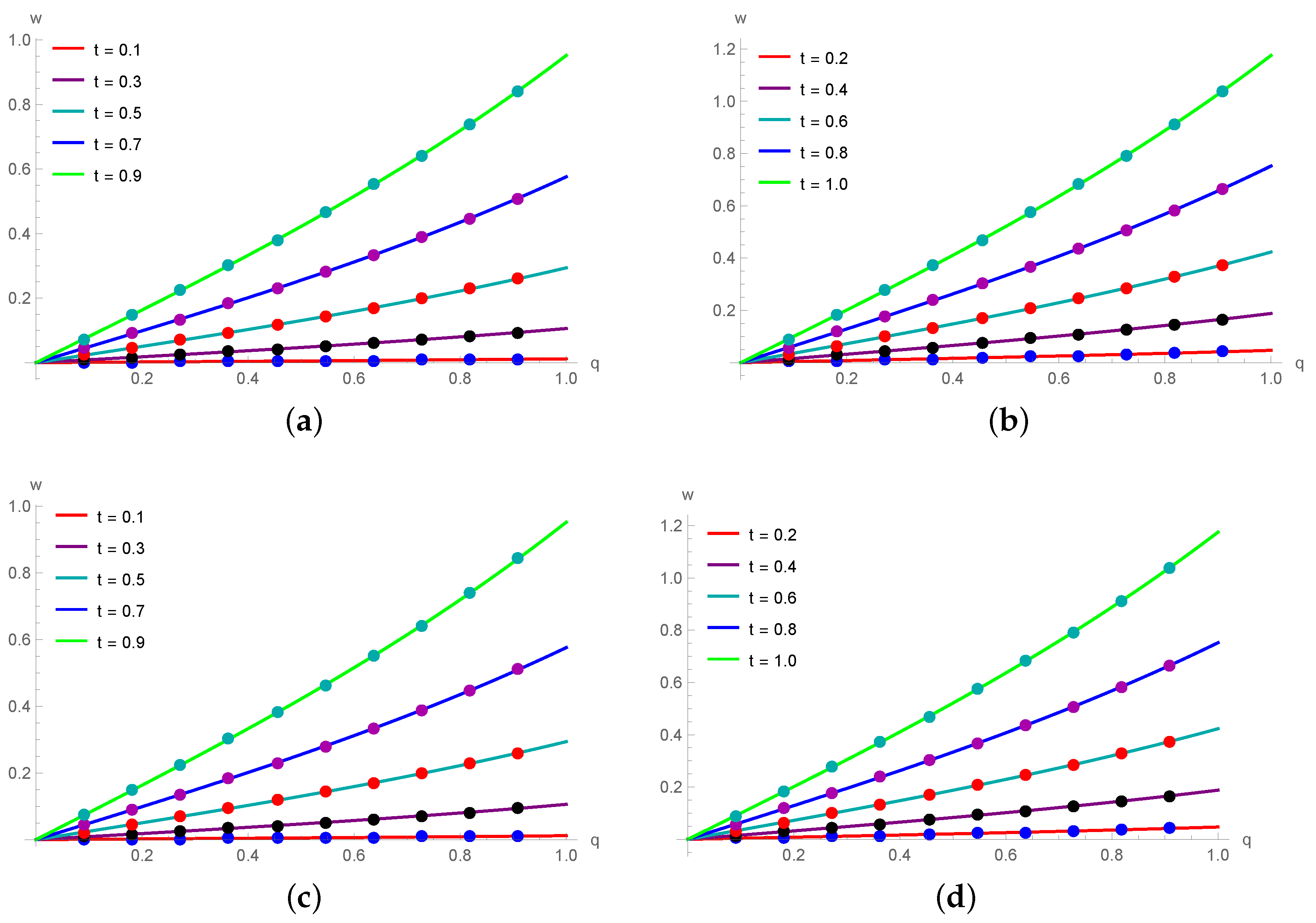
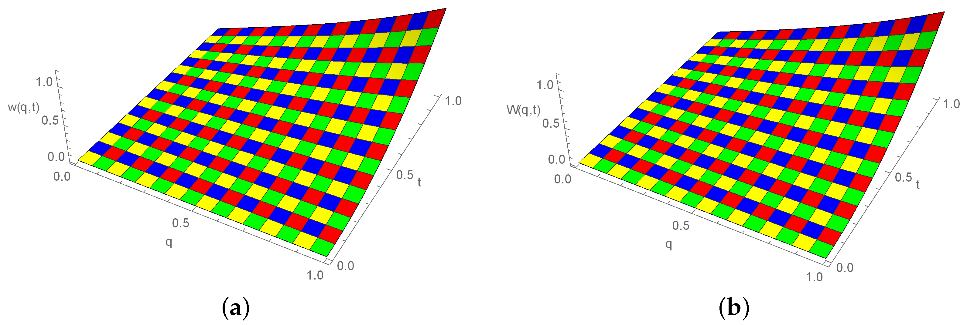
The expression w ( q , t ) = t 2 q ( 1 q ) is the exact solution. Table 8 contains the approximate results and the absolute errors for Example 2 at distinct spatial grid values. Table 9 describes the analysis of the convergence order and the error norms. For various time stages, the error norms L and L 2 are expressed in Table 10. Table 11 expounds the error norms at distinct values of Δ t . Figure 4 illustrates strong agreement between the approximative and analytical outcomes for different times. The 3D precision of the existing technique is shown by graphs of the analytic results and the numerical solutions in Figure 5. The graphs of the errors in 2D and 3D forms are displayed in Figure 6. The figures and tables depict that the proposed numerical results are compatible with the exact solutions. The piecewise CBS numerical solution for μ = 1.7 , N = 20 , Δ t = 0.001 and t = 1 for Example 2 is given in Equation (42).
W ( q , 1 ) = 4.14772 × 10 15 + q 1.00012 + 1.00000 0.000218646 q q , if   q [ 0.00 , 0.05 ) 2.62135 × 10 9 + q 1.00012 + 1.00000 0.000197675 q q , if   q [ 0.05 , 0.10 ) 2.4597 × 10 8 + q 1.00012 + 1.00001 0.0001757 q q , if   q [ 0.10 , 0.15 ) 1.00534 × 10 7 + q 1.00012 + 1.00002 0.0001532 q q , if   q [ 0.15 , 0.20 ) 2.84164 × 10 7 + q 1.00012 + 1.00003 0.000130246 q q , if   q [ 0.20 , 0.25 ) 6.48113 × 10 7 + q 1.00013 + 1.00005 0.000106953 q q , if   q [ 0.25 , 0.30 ) 1.28377 × 10 6 + q 1.00013 + 1.00007 0.0000834105 q q , if   q [ 0.30 , 0.35 ) 2.30071 × 10 6 + q 1.00014 + 1.0001 0.0000596917 q q , if   q [ 0.35 , 0.40 ) 3.82607 × 10 6 + q 1.00015 + 1.00013 0.000035858 q q , if   q [ 0.40 , 0.45 ) 6.00381 × 10 6 + q 1.00017 + 1.00016 0.0000119596 q q , if   q [ 0.45 , 0.50 ) 8.99371 × 10 6 + q 1.00018 + 1.00019 + 0.0000119596 q q , if   q [ 0.50 , 0.55 ) 1.29698 × 10 5 + q 1.00021 + 1.00023 + 0.000035858 q q , if   q [ 0.55 , 0.60 ) 1.81179 × 10 5 + q 1.00023 + 1.00028 + 0.0000596917 q q , if   q [ 0.60 , 0.65 ) 2.46317 × 10 5 + q 1.00026 + 1.00032 + 0.0000834105 q q , if   q [ 0.65 , 0.70 ) 3.27069 × 10 5 + q 1.0003 + 1.00037 + 0.000106953 q q , if   q [ 0.70 , 0.75 ) 4.25335 × 10 5 + q 1.00034 + 1.00042 + 0.000130246 q q , if   q [ 0.75 , 0.80 ) 5.42858 × 10 5 + q 1.00038 + 1.00048 + 0.0001532 q q , if   q [ 0.80 , 0.85 ) 6.81036 × 10 5 + q 1.00043 + 1.00054 + 0.0001757 q q , if   q [ 0.85 , 0.90 ) 8.41238 × 10 5 + q 1.00048 + 1.0006 + 0.000197675 q q , if   q [ 0.90 , 0.95 ) 0.000102104 + q 1.00054 + 1.00066 + 0.000218646 q q , if   q [ 0.95 , 1.00 ) .
Example 3.
Consider the TFDWE
μ w ( q , t ) t μ + w ( q , t ) 2 w ( q , t ) q 2 = p ( q , t ) , μ ( 1 , 2 ) , t [ 0 , 1 ] , q [ 0 , 1 ] ,
with ICs
w ( q , 0 ) = 0 , w t ( q , 0 ) = 0
and BCs
w ( 0 , t ) = 0 , w ( 1 , t ) = t 2 sinh ( 1 ) ,
where p ( q , t ) = 2 R ( μ ) 2 μ t sinh ( q ) E μ , 2 μ 2 μ t μ .
The expression w ( q , t ) = t 2 sinh ( q ) is the exact solution. Table 12 depicts the absolute error and computational outcomes for Example 3 at distinct spatial grid values. Comparison of the approximate solutions is demonstrated in Table 13. Table 14 expounds the absolute error for different μ values. Table 15 displays the analysis of the convergence order and the error norm in the spatial direction. Table 16 comprises the error norm for μ = 1.5 at numerous time stages. Table 17 describes the error norm at distinct values of Δ t . Figure 7 exhibits the relation between the numerical outcomes and the analytical results for distinct temporal directions. The 3D precision of the existing approach is displayed by graphs of the numerical results and the analytic solutions in Figure 8. Figure 9 demonstrates the 2D and 3D error descriptions.

7. Conclusions

This work dealt with the problem of determining numerical solutions for the time FPDE. A collocation approach using B-splines for the TFDWE was established for this purpose. This approach used the standard FDM to estimate the time fractional derivative, while the CuBS was utilized to discretize the space derivative. In order to evaluate the numerical solutions of the TFDWE combining damping and reaction components, an efficient numerical scheme was provided. Further, we employed the θ -weighted technique with ABFD. The suggested technique is stable unconditionally and exhibits second-order temporal and spatial convergence. Three numerical examples were investigated. The presented method is precise and computationally very efficient according to the numerical and graphical comparisons. In the future, we might think about using spline functions to solve higher-dimensional and variable-order FPDEs.

Author Contributions

Conceptualization, M.S. and M.A.; Funding acquisition, E.K.E.-S., M.A.E.A., N.F.A. and A.A.E.-R.; Investigation, M.S. and M.A.; Methodology, M.S. and M.A.; Project administration, E.K.E.-S., M.A.E.A., N.F.A. and A.A.E.-R.; Resources, M.A.; Software, M.S., M.A., M.A.E.A. and A.A.E.-R.; Supervision, M.A.; Validation, M.S., M.A., E.K.E.-S., M.A.E.A., N.F.A. and A.A.E.-R.; Writing—original draft, M.S., M.A., E.K.E.-S., M.A.E.A., N.F.A. and A.A.E.-R.; Writing—review and editing, M.S., E.K.E.-S., M.A.E.A., N.F.A. and A.A.E.-R. All authors have read and agreed to the published version of the manuscript.

Funding

The authors extend their appreciation to the Deputyship for Research & Innovation of the Ministry of Education of Saudi Arabia for funding this research work through project number 445-9-491.

Institutional Review Board Statement

Not applicable.

Informed Consent Statement

Not applicable.

Data Availability Statement

Data are contained within the article.

Acknowledgments

The authors extend their appreciation to the Deputyship for Research & Innovation, Ministry of Education of Saudi Arabia for funding this research work through project number 445-9-491. The authors are also grateful to the anonymous referees for their valuable suggestions, which significantly improved this manuscript.

Conflicts of Interest

The authors declare no conflict of interest.

References

  1. Leibniz, G.W. Letter from Hanover, Germany to G. F. A. L’Hospital, 30 September 1695; Mathematische Schriften 1849; Olms: Hidesheim, Germany, Reprinted 1962; pp. 301–302. [Google Scholar]
  2. Miller, K.S.; Ross, B. An Introduction to the Fractional Calculus and Fractional Differential Equations; Wiley: New York, NY, USA, 1993. [Google Scholar]
  3. Podlubny, I. Fractional Differential Equations: An Introduction to Fractional Derivatives, Fractional Differential Equations, to Methods of Their Solution and Some of Their Applications; Elsevier: Amsterdam, The Netherlands; Academic Press: San Diego, CA, USA, 1998; pp. 115–122. [Google Scholar]
  4. Magin, R.L. Fractional Calculus in Bioengineering; Begell House: Redding, CA, USA, 2006. [Google Scholar]
  5. Iftikhar, N.; Baleanu, D.; Riaz, M.B.; Husnine, S.M. Heat and mass transfer of natural convective flow with slanted magnetic field via fractional operators. J. Appl. Comput. Mech. 2021, 7, 189–212. [Google Scholar]
  6. Sokolov, I.M.; Klafter, J.; Blumen, A. Fractional kinetics. Phys. Today 2002, 55, 48–54. [Google Scholar] [CrossRef]
  7. Caputo, M.; Fabrizio, M. Damage and fatigue described by a fractional derivative model. J. Comput. Phys. 2015, 293, 400–408. [Google Scholar] [CrossRef]
  8. Atangana, A.; Bildik, N. The use of fractional order derivative to predict the groundwater flow. Math. Probl. Eng. 2013, 2013, 543026. [Google Scholar] [CrossRef]
  9. Atangana, A.; Vermeulen, P.D. Analytical solutions of a space-time fractional derivative of groundwater flow equation. Abstr. Appl. Anal. 2014, 2014, 381753. [Google Scholar] [CrossRef]
  10. Tenreiro Machado, J.A.; Silva, M.F.; Barbosa, R.S.; Jesus, I.S.; Reis, C.M.; Marcos, M.G.; Galhano, A.F. Some applications of fractional calculus in engineering. Math. Probl. Eng. 2010, 2010, 639801. [Google Scholar] [CrossRef]
  11. Metzler, R.; Jeon, J.H.; Cherstvy, A.G.; Barkai, E. Anomalous diffusion models and their properties: Non-stationarity, non-ergodicity, and ageing at the centenary of single particle tracking. Phys. Chem. Chem. Phys. 2014, 16, 24128–24164. [Google Scholar] [CrossRef]
  12. Karaman, M.M.; Sui, Y.; Wang, H.; Magin, R.L.; Li, Y.; Zhou, X.J. Differentiating low- and high-grade pediatric brain tumors using a continuous-time random-walk diffusion model at high b-values. Magn. Reson. Med. 2015, 76, 1149–1157. [Google Scholar] [CrossRef]
  13. Zhang, Y.; Baeumer, B.; Chen, L.; Reeves, D.M.; Sun, H. A fully subordinated linear flow model for hillslope subsurface stormflow. Water Resour. Res. 2017, 53, 3491–3504. [Google Scholar] [CrossRef]
  14. Tarasova, V.V.; Tarasov, V.E. Concept of dynamic memory in economics. Commun. Nonlinear Sci. Numer. Simul. 2018, 55, 127–145. [Google Scholar] [CrossRef]
  15. Boulaaras, S.; Rehman, Z.U.; Abdullah, F.A.; Jan, R.; Abdalla, M.; Jan, A. Coronavirus dynamics, infections and preventive interventions using fractional-calculus analysis. AIMS Math. 2023, 8, 8680–8701. [Google Scholar] [CrossRef]
  16. Bas, E.; Ozarslan, R. Real world applications of fractional models by Atangana-Baleanu fractional derivative. Chaos Solit. Fractals 2018, 116, 121–125. [Google Scholar] [CrossRef]
  17. Gómez-Aguilar, J.F.; Escobar-Jiménez, R.F.; López-López, M.G.; Alvarado-Martínez, V.M. Atangana-Baleanu fractional derivative applied to electromagnetic waves in dielectric media. J. Electromagn. Waves Appl. 2016, 30, 1937–1952. [Google Scholar]
  18. Ghanbari, B.; Atangana, A. A new application of fractional Atangana-Baleanu derivatives: Designing ABC-fractional masks in image processing. Phys. A Stat. Mech. Appl. 2020, 542, 123516. [Google Scholar] [CrossRef]
  19. Gao, W.; Ghanbari, B.; Baskonus, H.M. New numerical simulations for some real world problems with Atangana-Baleanu fractional derivative. Chaos Solitons Fractals 2019, 128, 34–43. [Google Scholar] [CrossRef]
  20. Ravichandran, C.; Logeswari, K.; Khan, A.; Abdeljawad, T.; Gómez-Aguilar, J.F. An epidemiological model for computer virus with Atangana-Baleanu fractional derivative. Results Phys. 2023, 51, 106601. [Google Scholar] [CrossRef]
  21. Hanif, A.; Butt, A.I.K. Atangana-Baleanu fractional dynamics of dengue fever with optimal control strategies. AIMS Math. 2023, 8, 15499–15535. [Google Scholar] [CrossRef]
  22. Goyal, M.; Saraswat, A.K.; Prakash, A. Numerical analysis of fractional coronavirus model with Atangana-Baleanu derivative in Liouville-Caputo sense. Ind. J. Phys. 2023, 97, 147–164. [Google Scholar] [CrossRef]
  23. Liu, Z.; Cheng, A.; Li, X. A novel finite difference discrete scheme for the time fractional diffusion-wave equation. Appl. Numer. Math. 2018, 134, 17–30. [Google Scholar] [CrossRef]
  24. Huang, J.; Tang, Y.; Vázquez, L.; Yang, J. Two finite difference schemes for time fractional diffusion-wave equation. Numer. Algorithms 2013, 64, 707–720. [Google Scholar] [CrossRef]
  25. Dehghan, M.; Abbaszadeh, M.; Mohebbi, A. Analysis of a meshless method for the time fractional diffusion-wave equation. Numer. Algorithms 2016, 73, 445–476. [Google Scholar] [CrossRef]
  26. Ali, U.; Iqbal, A.; Sohail, M.; Abdullah, F.A.; Khan, Z. Compact implicit difference approximation for time-fractional diffusion-wave equation. Alex. Eng. J. 2022, 61, 4119–4126. [Google Scholar] [CrossRef]
  27. Wei, L. Analysis of a new finite difference/local discontinuous Galerkin method for the fractional diffusion-wave equation. Appl. Math. Comput. 2017, 304, 180–189. [Google Scholar] [CrossRef]
  28. Soltani Sarvestani, F.; Heydari, M.H.; Niknam, A.; Avazzadeh, Z. A wavelet approach for the multi-term time fractional diffusion-wave equation. Int. J. Comput. Math. 2019, 96, 640–661. [Google Scholar] [CrossRef]
  29. Huang, J.; Yang, D.; Jay, L.O. Efficient methods for nonlinear time fractional diffusion-wave equations and their fast implementations. Numer. Algorithms 2020, 85, 375–397. [Google Scholar] [CrossRef]
  30. Fardi, M.; Al-Omari, S.K.Q.; Araci, S. A pseudo-spectral method based on reproducing kernel for solving the time-fractional diffusion-wave equation. Adv. Cont. Disc. Mod. 2022, 2022, 54. [Google Scholar] [CrossRef]
  31. Chen, J.; Liu, F.; Anh, V.; Shen, S.; Liu, Q.; Liao, C. The analytical solution and numerical solution of the fractional diffusion-wave equation with damping. Appl. Math. Comput. 2012, 219, 1737–1748. [Google Scholar] [CrossRef]
  32. Yang, J.Y.; Huang, J.F.; Liang, D.M.; Tang, Y.F. Numerical solution of fractional diffusion-wave equation based on fractional multistep method. Appl. Math. Model. 2014, 38, 3652–3661. [Google Scholar] [CrossRef]
  33. Chen, A.; Li, C. Numerical solution of fractional diffusion-wave equation. Numer. Funct. Anal. Optim. 2016, 37, 19–39. [Google Scholar] [CrossRef]
  34. Hashemi, M.S.; Inc, M.; Parto-Haghighi, M.; Bayram, M. On numerical solution of the time-fractional diffusion-wave equation with the fictitious time integration method. Eur. Phys. J. Plus 2019, 134, 488. [Google Scholar] [CrossRef]
  35. Shafiq, M.; Abbas, M.; Abualnaja, K.M.; Huntul, M.J.; Majeed, A.; Nazir, T. An efficient technique based on cubic B-spline functions for solving time-fractional advection diffusion equation involving Atangana-Baleanu derivative. Eng. Comput. 2022, 38, 901–917. [Google Scholar] [CrossRef] [PubMed]
  36. Abbas, M.; Bibi, A.; Alzaidi, A.S.M.; Nazir, T.; Majeed, A.; Akram, G. Numerical solutions of third-order time-fractional differential equations using cubic B-spline functions. Fractal Fract. 2022, 6, 528. [Google Scholar] [CrossRef]
  37. Dhiman, N.; Huntul, M.J.; Tamsir, M. A modified trigonometric cubic B-spline collocation technique for solving the time-fractional diffusion equation. Eng. Comput. 2021, 38, 2921–2936. [Google Scholar] [CrossRef]
  38. Shafiq, M.; Abbas, M.; Abdullah, F.A.; Majeed, A.; Abdeljawad, T.; Alqudah, M.A. Numerical solutions of time fractional Burgers’ equation involving Atangana-Baleanu derivative via cubic B-spline functions. Results Phys. 2022, 34, 105244. [Google Scholar] [CrossRef]
  39. Majeed, A.; Kamran, M.; Rafique, M. An approximation to the solution of time fractional modified Burgers’ equation using extended cubic B-spline method. Comput. Appl. Math. 2020, 39, 257. [Google Scholar] [CrossRef]
  40. Khader, M.M.; Abualnaja, K.M. Galerkin-FEM for obtaining the numerical solution of the linear fractional Klein-Gordon equation. J. Appl. Anal. Comput. 2019, 9, 261–270. [Google Scholar] [CrossRef]
  41. Majeed, A.; Kamran, M.; Iqbal, M.K.; Baleanu, D. Solving time fractional Burgers’ and Fisher’s equations using cubic B-spline approximation method. Adv. Differ. Equ. 2020, 2020, 175. [Google Scholar] [CrossRef]
  42. Shafiq, M.; Abdullah, F.A.; Abbas, M.; Alzaidi, A.S.M.; Riaz, M.B. Memory effect analysis using piecewise cubic B-spline of time fractional diffusion equation. Fractals 2022, 30, 2240270. [Google Scholar] [CrossRef]
  43. Poulin, J.R. Calculating Infinite Series Using Parseval’s Identity. Master’s Thesis, The University of Maine, Orono, ME, USA, 2020. [Google Scholar]
  44. Boyce, W.E.; Diprima, R.C.; Meade, D.B. Elementary Differential Equations and Boundary Value Problems; Wiley: New York, NY, USA, 1992. [Google Scholar]
  45. Kadalbajoo, M.K.; Arora, P. B-spline collocation method for the singular-perturbation problem using artificial viscosity. Comput. Math. Appl. 2009, 57, 650–663. [Google Scholar] [CrossRef]
  46. Hall, C.A. On error bounds for spline interpolation. J. Approx. Theory 1968, 1, 209–218. [Google Scholar] [CrossRef]
  47. De Boor, C. On the convergence of odd-degree spline interpolation. J. Approx. Theory 1968, 1, 452–463. [Google Scholar] [CrossRef]
  48. Khader, M.M.; Adel, M.H. Numerical solutions of fractional wave equations using an efficient class of FDM based on the Hermite formula. Adv. Differ. Equ. 2016, 2016, 34. [Google Scholar] [CrossRef]
  49. Avazzadeh, Z.; Hosseini, V.R.; Chen, W. Radial basis functions and FDM for solving fractional diffusion-wave equation. Iran. J. Sci. Technol. 2014, 38, 205–212. [Google Scholar]
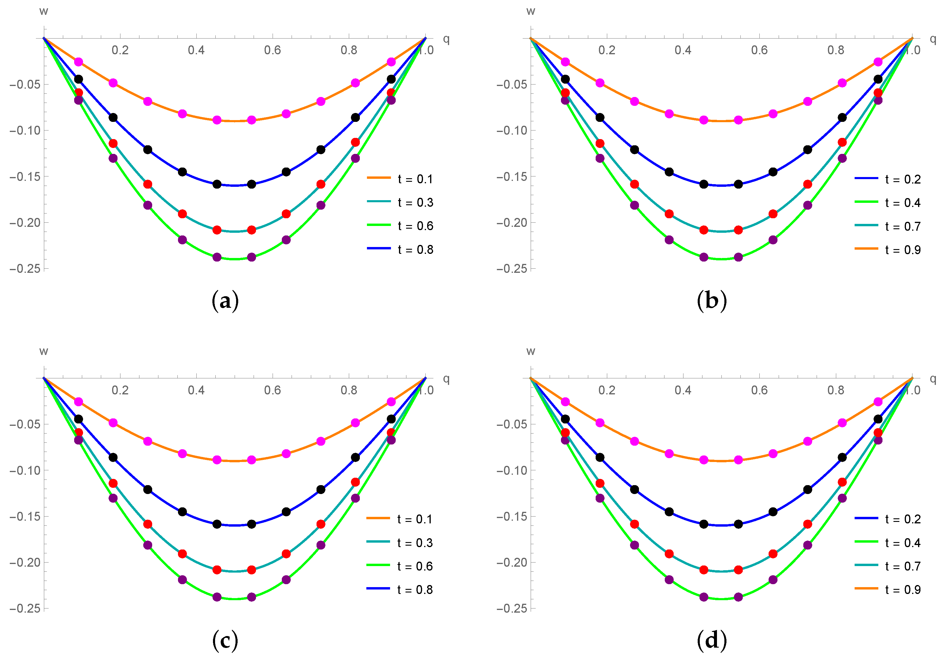
Figure 1. Exact results and approximate solutions at various temporal stages for Example 1. (a) N = 100 , μ = 1.8 and Δ t = 0.01 . (b) N = 100 , μ = 1.8 and Δ t = 0.01 . (c) N = 140 , μ = 1.3 and Δ t = 0.02 . (d) N = 140 , μ = 1.3 and Δ t = 0.02 .
Fractalfract 08 00018 g001
Figure 2. The 3D exact and numerical solutions for N = 64 , t = 1 , q [ 0 , 1 ] , Δ t = 0.01 and μ = 1.5 for Example 1. (a) Exact solution. (b) Numerical solution.
Fractalfract 08 00018 g002
Figure 3. The 2D and 3D error profiles for q [ 0 , 1 ] , N = 64 , μ = 1.5 , t = 1 and Δ t = 0.01 for Example 1. (a) 2D error function. (b) 3D error function.
Fractalfract 08 00018 g003
Figure 4. Exact and numerical solutions at different temporal stages with Δ t = 0.01 for Example 2. (a) N = 80 , μ = 1.5 . (b) N = 80 , μ = 1.5 . (c) N = 120 , μ = 1.9 . (d) N = 120 , μ = 1.9 .
Fractalfract 08 00018 g004
Figure 5. The 3D exact and numerical solutions with Δ t = 0.001 , N = 60 , μ = 1.5 , t = 1 and q [ 0 , 1 ] for Example 2. (a) Exact solution. (b) Numerical solution.
Fractalfract 08 00018 g005
Figure 6. The 2D and 3D error profiles for N = 60 , μ = 1.5 , q [ 0 , 1 ] , t = 1 and Δ t = 0.001 for Example 2. (a) 2D error function. (b) 3D error function.
Fractalfract 08 00018 g006
Figure 7. Exact results and approximate solutions at various time stages for Example 3. (a) N = 150 , μ = 1.2 and Δ t = 0.01 . (b) N = 150 , μ = 1.2 and Δ t = 0.01 . (c) N = 70 , μ = 1.7 and Δ t = 0.005 . (d) N = 70 , μ = 1.7 and Δ t = 0.005 .
Fractalfract 08 00018 g007
Figure 8. The 3D exact and approximate solutions for N = 50 , μ = 1.6 , t = 1 , Δ t = 0.01 and q [ 0 , 1 ] for Example 3. (a) Exact solution. (b) Approximate solution.
Fractalfract 08 00018 g008
Figure 9. The 2D and 3D error profiles for Example 3 for N = 50 , μ = 1.6 , q [ 0 , 1 ] , Δ t = 0.01 and t = 1 . (a) 2D error function. (b) 3D error function.
Fractalfract 08 00018 g009
Table 1. Comparison of references [35,36] with proposed method.
ProblemB-Spline FunctionFractional DerivativeFinite Difference Scheme
Reference [35]Time fractional
advection
diffusion equation
Cubic B-spline
functions
First-order
Atangana–Baleanu
fractional derivative
First-order implicit
finite difference scheme
Reference [36]Third-order time
fractional differential
equation
Cubic B-spline
functions
with new
approximations
Caputo fractional
derivative
Crank–Nicholson finite
difference scheme
Proposed MethodTime fractional
diffusion
wave equation
Cubic B-spline
functions
Second-order
Atangana–Baleanu
fractional derivative
Second-order implicit
finite difference scheme
Table 2. Absolute errors at t = 0.2 , μ = 1.8 , N = 500 and Δ t = 0.02 for Example 1.
qExact ResultApproximate ResultAbsolute Error
0.1 0.0494427190999916 0.0494426878107180 3.12893 × 10 8
0.2 0.0940456403667957 0.0940455807426410 5.96242 × 10 8
0.3 0.1294427190999916 0.1294426369956048 8.21044 × 10 8
0.4 0.1521690426072246 0.1521689460718402 9.65354 × 10 8
0.5 0.16 0.1599998984902868 1.01510 × 10 7
0.6 0.1521690426072246 0.1521689460633164 9.65439 × 10 8
0.7 0.1294427190999916 0.1294426369739889 8.21260 × 10 8
0.8 0.0940456403667957 0.0940455806985063 5.96683 × 10 8
0.9 0.0494427190999916 0.0494426877304619 3.13695 × 10 8
Table 3. Error norms for different time stages for Δ t = 0.01 and μ = 1.9 for Example 1.
L L 2
t N = 500 N = 200 N = 500 N = 200
0.2 5.69766 × 10 8 3.56106 × 10 7 4.02886 × 10 8 2.51805 × 10 7
0.4 2.24204 × 10 7 1.40128 × 10 6 1.58537 × 10 7 9.90854 × 10 7
0.6 5.13884 × 10 7 3.21177 × 10 6 3.63372 × 10 7 2.27107 × 10 6
0.8 9.09391 × 10 7 5.68367 × 10 6 6.43038 × 10 7 4.01896 × 10 6
1.0 1.31546 × 10 6 8.22154 × 10 6 9.30169 × 10 7 5.81350 × 10 6
Table 4. Error norms for Example 1 for distinct values of h when Δ t = 1 120 , μ = 1.5 and t = 1 .
N L L 2 OrderCPU Time (s)
10 0.001501849010 0.001061967620 0.89063
20 3.78276 × 10 4 2.67481 × 10 4 1.989229 2.26563
40 9.47448 × 10 5 6.69947 × 10 5 1.997321 4.01563
80 2.36972 × 10 5 1.67564 × 10 5 1.999331 11.4375
160 5.92499 × 10 6 4.18959 × 10 6 1.999833 39.3594
Table 5. Error norm comparison for distinct values of h and Δ t for Example 1 for t = 0.2 and μ = 1.5 .
HF [48]Proposed Method
h Δ t L L L 2
1 5 1 50 0.01149 0.001950960729 0.001450531633
1 10 1 100 0.00361 5.23274 × 10 4 3.70011 × 10 4
1 20 1 150 0.00120 1.31762 × 10 4 9.31699 × 10 5
1 30 1 150 0.00115 5.85545 × 10 5 4.14043 × 10 5
1 30 1 200 0.00021 5.87875 × 10 5 4.15691 × 10 5
1 40 1 200 0.00019 3.30667 × 10 5 2.33817 × 10 5
1 40 1 210 0.00006 3.30857 × 10 5 2.33951 × 10 5
1 45 1 220 0.00004 2.61392 × 10 5 1.84945 × 10 5
Table 6. Error norm comparison for distinct values of h and Δ t for Example 1 for t = 0.4 and μ = 1.7 .
HF [48]Proposed Method
h Δ t L L L 2
1 10 1 50 0.01396 0.001082932435 7.65749 × 10 4
1 20 1 100 0.01064 2.74762 × 10 4 1.94286 × 10 4
1 30 1 200 0.00736 1.23063 × 10 4 8.70190 × 10 5
1 50 1 250 0.00653 4.43721 × 10 5 3.13758 × 10 5
1 50 1 300 0.00586 4.44191 × 10 5 3.14090 × 10 5
1 60 1 400 0.00494 3.08875 × 10 5 2.18407 × 10 5
1 60 1 450 0.00460 3.09012 × 10 5 2.18504 × 10 5
1 70 1 480 0.00443 2.27079 × 10 5 1.60569 × 10 5
Table 7. Error norms for distinct values of Δ t for Example 1 for μ = 1.5 and t = 1 .
Δ t h = ( Δ t ) 2 L L 2
1 4 1 16 3.75102 × 10 4 2.65237 × 10 4
1 8 1 64 3.01303 × 10 5 2.13053 × 10 5
1 16 1 256 2.11110 × 10 6 1.49277 × 10 6
1 32 1 1024 1.39222 × 10 7 9.84449 × 10 8
Table 8. Absolute error at t = 0.1 , N = 10 and Δ t = 0.0001 for Example 2.
Approximate ResultAbsolute Error
q Exact Result μ = 1.9 μ = 1.5 μ = 1.9 μ = 1.5
0.1 0.000900000000 0.000900042382 0.000900146277 4.23821 × 10 8 1.46277 × 10 7
0.2 0.001600000000 0.001600077842 0.001600273755 7.78422 × 10 8 2.73755 × 10 7
0.3 0.002100000000 0.002100103582 0.002100370496 1.03582 × 10 7 3.70496 × 10 7
0.4 0.002400000000 0.002400119048 0.002400430339 1.19048 × 10 7 4.30339 × 10 7
0.5 0.002500000000 0.002500124200 0.002500450539 1.24200 × 10 7 4.50539 × 10 7
0.6 0.002400000000 0.002400119048 0.002400430339 1.19048 × 10 7 4.30339 × 10 7
0.7 0.002100000000 0.002100103582 0.002100370496 1.03582 × 10 7 3.70496 × 10 7
0.8 0.001600000000 0.001600077842 0.001600273755 7.78422 × 10 8 2.73755 × 10 7
0.9 0.000900000000 0.000900042382 0.000900146277 4.23821 × 10 8 1.46277 × 10 7
Table 9. Error norms for Example 2 at various h values when t = 1 and μ = 1.5 .
h Δ t = h 2 L L 2 OrderCPU Time (s)
1 4 1 16 0.001737001774 0.001230987613 0.04688
1 8 1 64 4.58243 × 10 4 3.25090 × 10 4 1.922415 0.29688
1 16 1 256 1.16081 × 10 4 8.23743 × 10 5 1.980978 4.23438
1 32 1 1024 2.91155 × 10 5 2.06626 × 10 5 1.995277 187.781
Table 10. Error norms for different time stages with Δ t = 0.001 , N = 10 and μ = 1.9 for Example 2.
t L L 2
0.2 2.89129 × 10 6 2.08301 × 10 6
0.4 8.76628 × 10 6 6.27643 × 10 6
0.6 1.92499 × 10 5 1.37256 × 10 5
0.8 3.40618 × 10 5 2.42064 × 10 5
1.0 5.08449 × 10 5 3.60397 × 10 5
Table 11. Error norms for Example 2 at distinct values of Δ t = 1 M for μ = 1.3 , N = 10 and t = 1 .
M L L 2
10 0.002570857778 0.001824491691
20 0.001293829254 9.18167 × 10 4
40 6.48523 × 10 4 4.60211 × 10 4
80 3.24584 × 10 4 2.30330 × 10 4
160 1.62360 × 10 4 1.15212 × 10 4
Table 12. Absolute error for Example 3 for distinct choices of μ for Δ t = 0.01 and N = 400 at t = 1 .
Approximate SolutionAbsolute Error
q Exact Solution μ = 1.25 μ = 1.75 μ = 1.25 μ = 1.75
0.1 0.100166750020 0.100166742946 0.100166744812 7.07383 × 10 9 5.20813 × 10 9
0.2 0.201336002541 0.201335989089 0.201335992250 1.34525 × 10 8 1.02913 × 10 8
0.3 0.304520293447 0.304520274287 0.304520278486 1.91598 × 10 8 1.49610 × 10 8
0.4 0.410752325803 0.410752301987 0.410752306857 2.38155 × 10 8 1.89463 × 10 8
0.5 0.521095305494 0.521095278504 0.521095283598 2.69901 × 10 8 2.18956 × 10 8
0.6 0.636653582148 0.636653553958 0.636653558797 2.81898 × 10 8 2.33512 × 10 8
0.7 0.758583701840 0.758583675002 0.758583679117 2.68376 × 10 8 2.27226 × 10 8
0.8 0.888105982188 0.888105959935 0.888105962924 2.22522 × 10 8 1.92641 × 10 8
0.9 1.026516725708 1.026516712082 1.026516713651 1.36261 × 10 8 1.20571 × 10 8
Table 13. Comparison of approximate solutions for Example 3 μ = 1.5 for N = 50 at t = 1 .
M = 10M = 50
q Exact Solution RBF [49] Proposed Method RBF [49] Proposed Method
0.1 0.10016675 0.09950933 0.10016634 0.09951107 0.10016634
0.2 0.20133600 0.20079972 0.20133520 0.20080291 0.20133521
0.3 0.30452029 0.30402685 0.30451914 0.30403116 0.30451915
0.4 0.41075233 0.41029949 0.41075088 0.41030448 0.41075090
0.5 0.52109531 0.52065615 0.52109366 0.52066138 0.52109368
0.6 0.63665358 0.63621617 0.63665186 0.63622115 0.63665187
0.7 0.75858370 0.75812244 0.75858205 0.75812672 0.75858206
0.8 0.88810598 0.88761746 0.88810461 0.88762062 0.88810462
0.9 1.02651673 1.02593218 1.02651588 1.02593389 1.02651588
1.0 1.17520119 1.17520119 1.17520119 1.17520119 1.17520119
Table 14. Absolute error for Example 3 for distinct choices of μ for Δ t = 0.0001 and N = 100 at t = 0.1 .
q μ = 1.2 μ = 1.4 μ = 1.6 μ = 1.8
0.1 2.25149 × 10 10 1.68967 × 10 10 1.12538 × 10 10 5.62889 × 10 11
0.2 4.50977 × 10 10 3.39147 × 10 10 2.26151 × 10 10 1.13141 × 10 10
0.3 6.77001 × 10 10 5.11198 × 10 10 3.41799 × 10 10 1.71124 × 10 10
0.4 8.99801 × 10 10 6.84174 × 10 10 4.59985 × 10 10 2.30803 × 10 10
0.5 1.10981 × 10 09 8.53206 × 10 10 5.79669 × 10 10 2.92657 × 10 10
0.6 1.28547 × 10 09 1.00456 × 10 09 6.95165 × 10 10 3.56519 × 10 10
0.7 1.38305 × 10 09 1.10574 × 10 09 7.88129 × 10 10 4.18704 × 10 10
0.8 1.31947 × 10 09 1.08677 × 10 09 8.08813 × 10 10 4.60023 × 10 10
0.9 9.44813 × 10 10 8.07071 × 10 10 6.36143 × 10 10 4.04391 × 10 10
Table 15. Error norms for Example 3 for distinct values of h when t = 1 and μ = 1.7 .
h Δ t = h 2 L L 2 OrderCPU Time (s)
1 4 1 16 2.38724 × 10 4 1.79685 × 10 4 0.07813
1 8 1 64 6.13836 × 10 5 4.37651 × 10 5 1.959420 0.34375
1 16 1 256 1.52289 × 10 5 1.08588 × 10 5 2.011043 6.48438
1 32 1 1024 3.79989 × 10 6 2.70939 × 10 6 2.002782 192.672
Table 16. Error norms for Δ t = 0.01 , N = 500 and μ = 1.5 for Example 3 at various time stages.
t L L 2
0.2 2.72263 × 10 10 1.88811 × 10 10
0.4 1.69968 × 10 09 1.20289 × 10 09
0.6 4.82802 × 10 09 3.44298 × 10 09
0.8 9.93347 × 10 09 7.09972 × 10 09
1.0 1.71278 × 10 08 1.22658 × 10 08
Table 17. Error norms for Example 3 for distinct values of Δ t for t = 1 and μ = 1.3 .
Δ t h = ( Δ t ) 2 L L 2
1 4 1 16 1.76015 × 10 5 1.26352 × 10 5
1 8 1 64 1.09565 × 10 6 7.84619 × 10 7
1 16 1 256 6.82729 × 10 8 4.88769 × 10 8
1 32 1 1024 4.14100 × 10 9 2.91889 × 10 9
Disclaimer/Publisher’s Note: The statements, opinions and data contained in all publications are solely those of the individual author(s) and contributor(s) and not of MDPI and/or the editor(s). MDPI and/or the editor(s) disclaim responsibility for any injury to people or property resulting from any ideas, methods, instructions or products referred to in the content.