Article

Proposal for Use of the Fractional Derivative of Radial Functions in Interpolation Problems

by
Anthony Torres-Hernandez
1,2,*,
Fernando Brambila-Paz
3 and
Rafael Ramirez-Melendez
2
1
Department of Physics, Faculty of Science, Universidad Nacional Autónoma de México, Mexico City 04510, Mexico
2
Music and Machine Learning Lab, Department of Information and Communication Technologies, Universitat Pompeu Fabra, 08018 Barcelona, Spain
3
Department of Mathematics, Faculty of Science, Universidad Nacional Autónoma de México, Mexico City 04510, Mexico
*
Author to whom correspondence should be addressed.
Fractal Fract. 2024, 8(1), 16; https://doi.org/10.3390/fractalfract8010016
Submission received: 10 November 2023 / Revised: 6 December 2023 / Accepted: 17 December 2023 / Published: 23 December 2023

Abstract

:
This paper presents the construction of a family of radial functions aimed at emulating the behavior of the radial basis function known as thin plate spline (TPS). Additionally, a method is proposed for applying fractional derivatives, both partially and fully, to these functions for use in interpolation problems. Furthermore, a technique is employed to precondition the matrices generated in the presented problems through Q R decomposition. Similarly, a method is introduced to define two different types of abelian groups for any fractional operator defined in the interval [ 0 , 1 ) , among which the Riemann–Liouville fractional integral, Riemann–Liouville fractional derivative, and Caputo fractional derivative are worth mentioning. Finally, a form of radial interpolant is suggested for application in solving fractional differential equations using the asymmetric collocation method, and examples of its implementation in differential operators utilizing the aforementioned fractional operators are shown.

1. Introduction

Radial basis functions (RBFs) have become instrumental in various mathematical and computational domains, stemming from the necessity to address challenges in multivariate interpolation and partial differential equations (PDEs) when dealing with randomly distributed, scattered data points, as encountered in cartography. The pioneering contribution of Hardy marked the inception of a research area that has significantly evolved [1]. Coined by Kansa in the 1990s, the term “radial basis functions” traces its development back to earlier works in the 1970s by Micchelli, Powell, and other researchers exploring the nonsingularity theorem [2,3]. Kansa’s proposal to consider analytical derivatives of RBFs paved the way for numerical schemes in solving PDEs [4,5], proving valuable in higher-dimensional and irregular domains.
The power of RBFs lies in their ability to achieve accurate interpolation and approximation in cases where traditional grids and structured approaches are not feasible. The unique flexibility of RBFs in the choice of functions, allowing adaptation to various problems and applications across scientific and engineering fields, boosts their ongoing development and refinement. Applications of RBFs extend into diverse domains, including physics, engineering, complex systems modeling, data science, and more [6,7,8,9]. In computational physics, RBFs play a crucial role in solving partial differential equations that describe natural phenomena like fluid flow and wave propagation. In engineering, they serve as valuable tools for designing and analyzing structures, enabling the precise simulation of complex behaviors. Additionally, RBFs find applications in data science and machine learning tasks, such as data interpolation, approximation, and pattern detection in multidimensional datasets.
Within the realm of radial basis functions, various types of radial functions have been proposed for different applications. Examples include polyharmonic splines, multiquadric functions, inverse multiquadric functions, and Gaussian functions, with each serving different purposes [10,11]. Despite their advantages, the matrices resulting from methods involving RBFs can be dense and suffer from ill-conditioning, leading to numerical challenges. Additionally, some RBFs have a shape parameter that significantly impacts the accuracy of numerical results, influencing the interpolation and approximation process. To tackle these challenges and enhance the conditioning of interpolation matrices, alternative algorithms have been developed. Examples include the Contour–Padé method, proposed by Fornberg and Wright [12], which generates better-conditioned interpolants, and the RBF-QR method, introduced by Fornberg and Piret [13], using Q R matrix decomposition to transform function bases into well-conditioned ones.
In the realm of fractional calculus, a fractional derivative generalizes the ordinary derivative, and fractional differential equations involve operators of fractional order, becoming increasingly essential in various research areas, including magnetic field theory, fluid dynamics, electrodynamics, and multidimensional processes [14,15,16,17]. Fractional operators find applications in finance, economics, the Riemann zeta function, and the study of hybrid solar receivers [18,19,20,21,22,23]. Furthermore, the study of fractional operators has expanded to include solving nonlinear algebraic systems [24,25,26,27,28,29,30].
Due to the importance of fractional differential equations, numerous numerical methods have been proposed, with radial basis functions standing out due to their independence from problem dimensions and their meshless characteristics [31,32,33,34]. The acquisition of precise solutions for differential equations, both classical and fractional, remains fundamental in engineering and computational mathematics. In this context, the thin plate spline (TPS), a radial basis function defined as follows [10]:
Φ ( r ) = r n log ( r ) , n 2 N ,
emerges as a versatile tool for modeling various behaviors. However, its direct application faces challenges that require meticulous adaptations to address specific domains and problems. To exemplify one of the challenges of directly applying the TPS function, it is considered an m-th derivative, which may be written in general form as follows:
Φ ( m ) ( r ) = r n m Γ n + 1 Γ n m + 1 log ( r ) + 1 δ m , 0 k = 1 m ( 1 ) k + 1 k Γ n + 1 Γ m + 1 Γ n m + k + 1 Γ m k + 1 ,
where Γ ( · ) and δ m , 0 denote the Gamma function and the Kronecker delta, respectively. So, it should be noted that when m n , the previous function presents singularities whenever r is equal to zero, the consequences of which include obtaining interpolation matrices that may be analytically invertible but numerically singular when 0 < r 1 . This phenomenon is usually associated with the ill-conditioning of the matrices. Ill-conditioned matrices have eigenvalues very close to zero, making the numerical inversion process very sensitive to computational errors. Then, when the TPS function is applied directly, significant obstacles may arise when dealing with particular problems that demand a more specific approach. These challenges may stem from the complexity of certain domains or from the inherent characteristics of the differential equations to be solved. In response to these challenges, this paper focuses on building a family of radial functions designed to emulate and extend the behavior of the TPS function. This approach provides a flexible and adaptable alternative, allowing, in some cases, addressing the limitations associated with direct application of the aforementioned function. Rather than solely relying on a specific function, the proposed family of radial functions aims to more effectively address the inherent complexity of differential problems in various domains, including those involving fractional operators, even in multiple dimensions [31].

2. Polynomials with Similar Behavior to the TPS Function

This section begins with a simple but fundamental objective for subsequent results, which is to extend the behavior of the TPS function within a domain Ω of the type:
Ω = [ 0 , 1 ] × [ 0 , 1 ] ,
into a domain of the following form:
Ω b = [ 0 , b ] × [ 0 , b ] .
For this purpose, it is essential to consider that Equation (1) fulfills the following:
Φ ( 0 ) = 0 , Φ ( 0 ) = 0 , Φ ( 1 ) = 0 , Φ ( 1 ) = 1 .
Therefore, a radial function Φ ( r ) that fulfills the following is sought:
Φ ( 0 ) = 0 , Φ ( 0 ) = 0 ,
Φ ( b ) = 0 , Φ ( b ) = 1 .
To fulfill the conditions outlined in Equation (3), a polynomial of the following form is considered:
Φ ( r ) = a 1 r N + 1 + a 0 r N ,
where the coefficients a 0 and a 1 are determined using Equation (4). The value of N will be determined later. Subsequently:
Φ ( b ) = a 1 b N + 1   +   a 0 b N   = 0 , Φ ( b ) = a 1 ( N + 1 ) b N + a 0 N b N 1 = 1 .
In matrix form, the system above may be represented as
b N + 1 b N ( N + 1 ) b N N b N 1 B a 1 a 0 a = 0 1 c .
Let d e t ( B ) be the determinant of the matrix B from the previous system. Performing some algebraic operations, it is obtained that:
d e t ( B ) = b 2 N 0 b 0 .
Hence, for the system (5), a solution always exists. Let a d j ( B ) be the adjoint matrix of matrix B. So, using the following equality:
B 1 = 1 d e t ( B ) a d j ( B ) ,
it is obtained that
B 1 = N b 1 N b N ( N + 1 ) b N b 1 N .
Then, the solution to the system (5) is given by
a 1 a 0 = b N b 1 N .
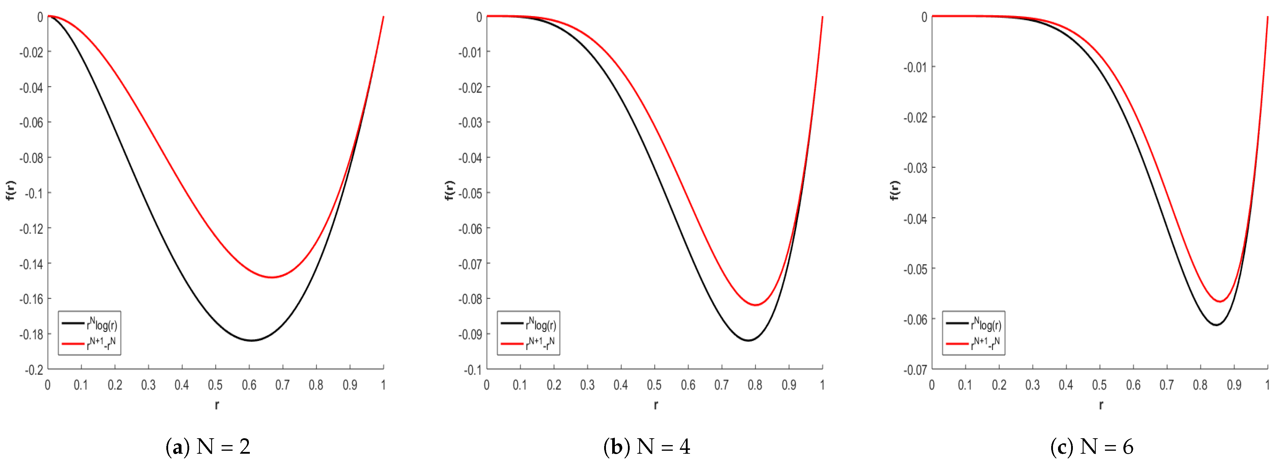
As a consequence, the following polynomial is obtained:
Φ ( N , r ) = b N r N + 1 b 1 N r N .
Through the previous construction, Equation (7) in the domain Ω 1 fulfills the following (see Figure 1):
Φ ( N , r ) = r N + 1 r N r N log ( r ) ,
In the previous construction, only two coefficients were used to approximate the TPS function. To introduce one more coefficient, it is considered that Equation (1) in the domain Ω 1 fulfills the following:
Φ ( 0 ) = 0 , Φ ( 0 ) = 0 , Φ ( 0 ) = 0 Φ ( 1 ) = 0 , Φ ( 1 ) = 1 , Φ ( 1 ) = 2 n 1 .
As a consequence, a radial function Φ ( r ) is sought to fulfill the following:
Φ ( 0 ) = 0 , Φ ( 0 ) = 0 , Φ ( 0 ) = 0 ,
Φ ( b ) = 0 , Φ ( b ) = 1 , Φ ( b ) = 2 N 1 .
To fulfill Equation (8), the following polynomial is chosen:
Φ ( r ) = a 2 r N + 2 + a 1 r N + 1 + a 0 r N ,
and to fulfill Equation (9), the following matrix system is obtained:
b N + 2 b N + 1 b N ( N + 2 ) b N + 1 ( N + 1 ) b N N b N 1 ( N + 2 ) ( N + 1 ) b N ( N + 1 ) N b N 1 N ( N 1 ) b N 2 B a 2 a 1 a 0 a = 0 1 2 N 1 c .
After some algebraic manipulation, it is obtained that
det ( B ) = 2 b 3 N 0 b 0 ,
So, using Equation (6), it is obtained that
B 1 = 1 2 N ( N + 1 ) b 2 N N b 1 N 1 2 b N N ( N + 2 ) b 1 N ( 2 N + 1 ) b N b 1 N 1 2 N 2 + 3 N + 2 b N ( N + 1 ) b 1 N 1 2 b 2 N .
Therefore, system (10) has the following solution:
a 2 a 1 a 0 = 1 2 ( 2 N 1 ) b N N b N 1 ( 2 N + 1 ) b N ( 2 N 1 ) b 1 N 1 2 ( 2 N 1 ) b 2 N ( N + 1 ) b 1 N .
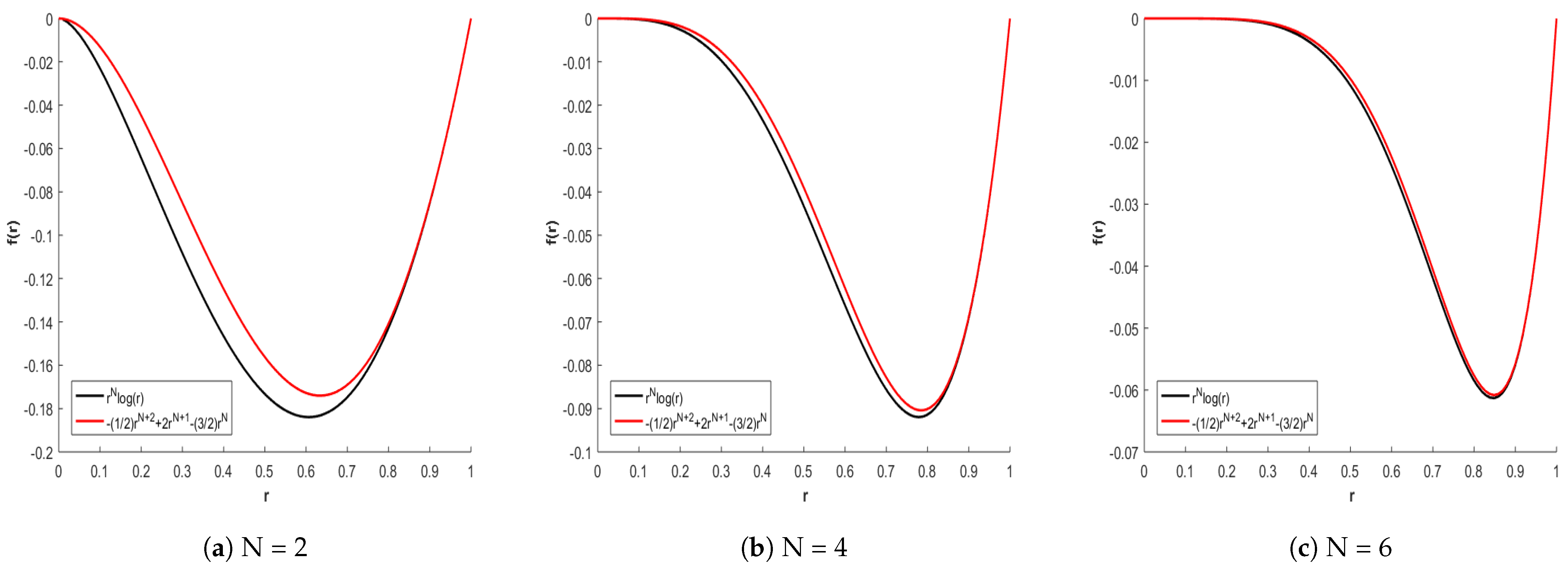
This results in the following polynomial:
Φ ( N , r ) = 1 2 ( 2 N 1 ) b N N b N 1 r N + 2 + ( 2 N + 1 ) b N ( 2 N 1 ) b 1 N r N + 1 + 1 2 ( 2 N 1 ) b 2 N ( N + 1 ) b 1 N r N .
Thus, through the previous construction, Equation (11) in the domain Ω 1 fulfills the following (see Figure 2):
Φ ( N , r ) = 1 2 r N + 2 + 2 r N + 1 3 2 r N r N log ( r ) .
From the matrix systems given in Equations (5) and (10), it may be deduced that to construct a polynomial with n coefficients that approximates the TPS function, it is necessary to consider the ( n 1 ) derivatives of both the polynomial and the TPS function. However, this approach would lead to more complex expressions for the coefficients a i . In the next section, an alternative method is presented that allows obtaining an approximation for the TPS function while keeping the coefficients a i in a simpler form.

2.1. Pseudo TPS Function

In pursuit of subsequently employing the fractional derivatives of polynomials [35], while preserving the TPS function’s behavior of being zero at the boundaries of the domain Ω 1 , the approach begins by seeking a polynomial that becomes zero, along with its derivatives, at the boundaries of the proposed domain. Directly solving the system (5) with the mentioned conditions leads to a trivial solution. Instead, the polynomial involved in the system (10) is considered with a vector c of the form:
c = 0 0 c 0 ,
where c 0 > 0 and the minus sign is included to ensure that the solution exhibits a convex behavior analogous to the TPS function in the domain Ω 1 . With these considerations, the system (10) may be rewritten as
b N + 2 b N + 1 b N ( N + 2 ) b N + 1 ( N + 1 ) b N N b N 1 ( N + 2 ) ( N + 1 ) b N ( N + 1 ) N b N 1 N ( N 1 ) b N 2 B a 2 a 1 a 0 a = 0 0 c 0 c .
This system has the following solution:
a 2 a 1 a 0 = 1 2 c 0 b N c 0 b 1 N 1 2 c 0 b 2 N ,
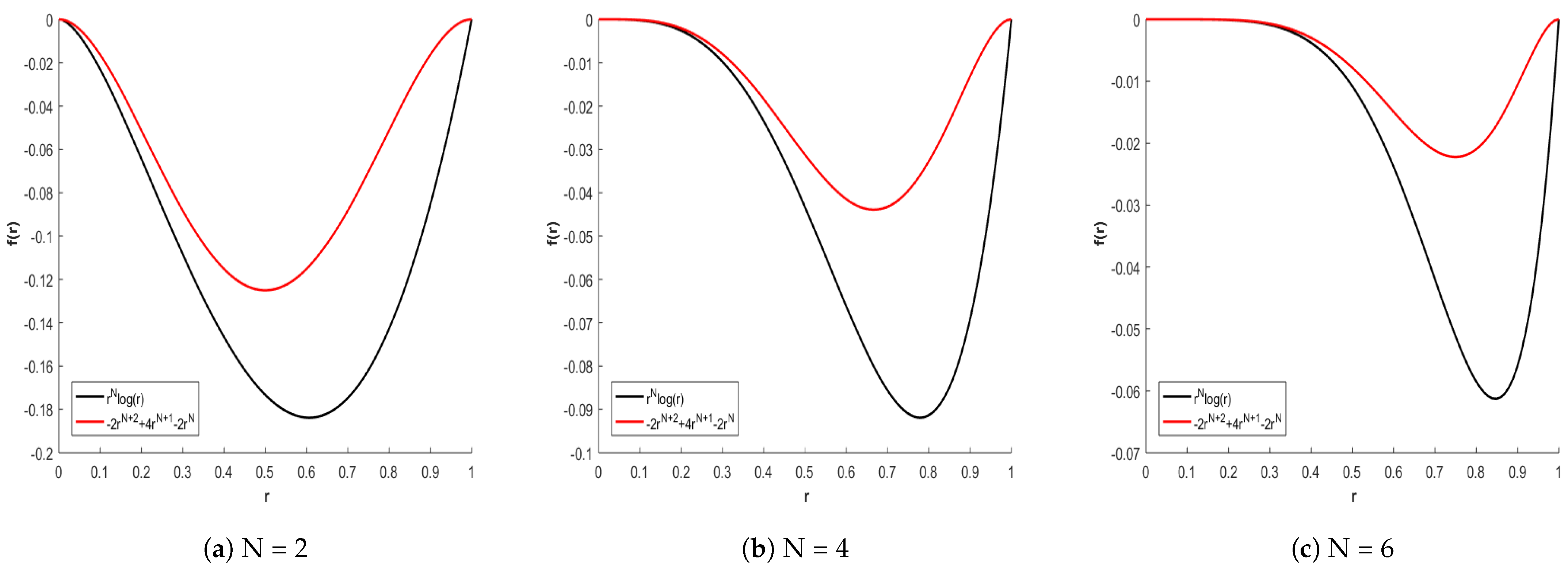
which generates the polynomial:
Φ ( N , r ) = c 0 2 b N r N + 2 + c 0 b 1 N r N + 1 c 0 2 b 2 N r N .
Although c 0 may be chosen arbitrarily, a method is subsequently proposed to select its value in such a way that the coefficients of the polynomial (
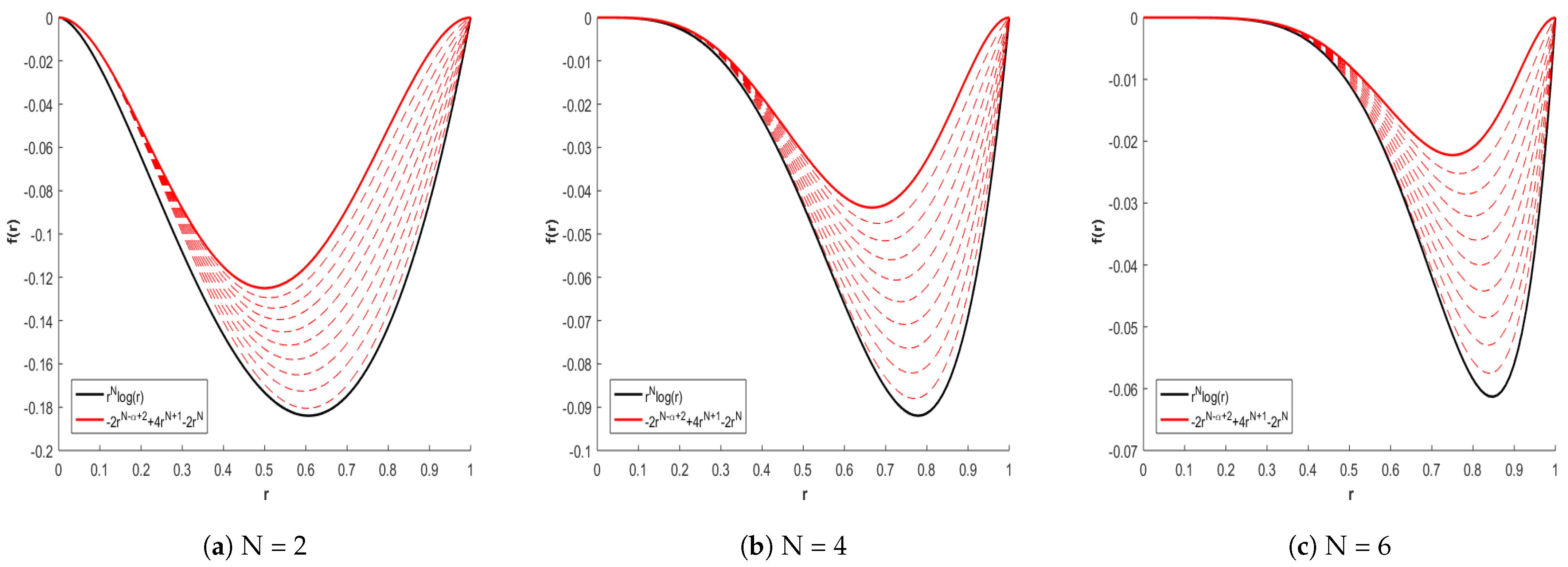
13) remain simple. For the specific case of c 0 = 4 , the following polynomial is obtained:
Φ ( N , r ) = 2 b N r N + 2 + 4 b 1 N r N + 1 2 b 2 N r N ,
Thus, the choice of c 0 and the construction of the polynomial (14) ensure that, in the domain Ω 1 , it fulfills the following (see Figure 3):
Φ ( N , r ) = 2 r N + 2 + 4 r N + 1 2 r N r N log ( r ) .
To enhance the approximation, a small perturbation α , where α [ 0 , 1 ) , is introduced in the exponent of the term with the highest power associated with a negative coefficient. Simultaneously, the exponent of said coefficient is adjusted by adding a perturbation + α . For the aforementioned case, this allows defining the following function:
Φ ( α , N , r ) = 2 b N + α r N α + 2 + 4 b 1 N r N + 1 2 b 2 N r N ,
which in the domain Ω 1 fulfills the following (see Figure 4):
Φ ( α , N , r ) = 2 r N α + 2 + 4 r N + 1 2 r N r N log ( r ) .
To conclude this section, it is worth mentioning that Equation (16) is referred to as the pseudo TPS function, while Equation (15) is referred to as the generalized pseudo TPS function.

2.2. Generalizing the Previous Construction

To extend the previous process used in constructing the pseudo TPS function, this begins by employing a polynomial of the following form:
Φ ( r ) = a 3 r N + 3 + a 2 r N + 2 + a 1 r N + 1 + a 0 r N ,
such that its coefficients fulfill the following conditions:
Φ ( b ) = 0 , Φ ( b ) = 0 , Φ ( b ) = 0 , Φ ( b ) = c 0 .
This leads to a matrix system of the form B a = c , where the vector c has the following form:
c = 0 0 0 c 0 ,
and the determinant of matrix B fulfills the following:
det ( B ) = 12 b 4 N 0 b 0 .
Therefore, using Equation (6), it is obtained that
B 1 = B 3 1 B 2 1 B 1 1 B 0 1 ,
where B i 1 i = 0 3 are the column vectors of the inverse matrix of B, with
B 0 1 = 1 6 b N   1 2 b 1 N 1 2 b 2 N 1 6 b 3 N .
Then, the previous matrix system has the following solution:
a = c 0 6 b N c 0 2 b 1 N c 0 2 b 2 N c 0 6 b 3 N ,
with which the following polynomial is obtained:
Φ ( N , r ) = c 0 6 b N r N + 3 c 0 2 b 1 N r N + 2 + c 0 2 b 2 N r N + 1 c 0 6 b 3 N r N .
Let M be the least common multiple (LCM) of the denominators in the coefficients of polynomial (17). Consequently, the value of c 0 is defined as follows:
c 0 = p M , p Z 0 ,
where
p > 0 , if Φ ( 2 , r ) is convex in Ω 1 p < 0 , if Φ ( 2 , r ) is concave in Ω 1 .
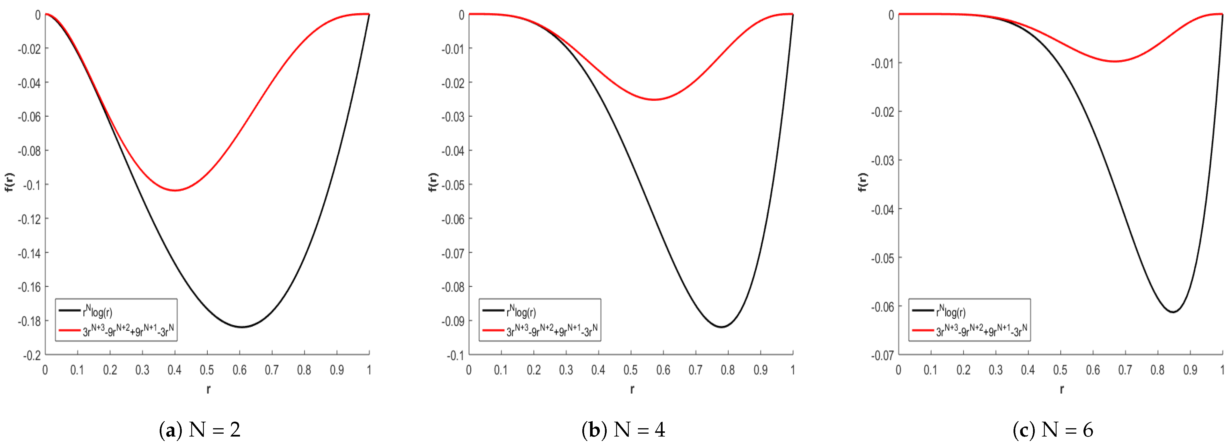
To exemplify the previous approximation, it is possible to choose the value c 0 = 18 in Equation (17), resulting in the following polynomial:
Φ ( N , r ) = 3 b N r N + 3 9 b 1 N r N + 2 + 9 b 2 N r N + 1 3 b 3 N r N .
Due to the choice of c 0 and the way in which the function (18) is constructed, in the domain Ω 1 , it fulfills the following (see Figure 5):
Φ ( N , r ) = 3 r N + 3 9 r N + 2 + 9 r N + 1 3 r N r N log ( r ) .
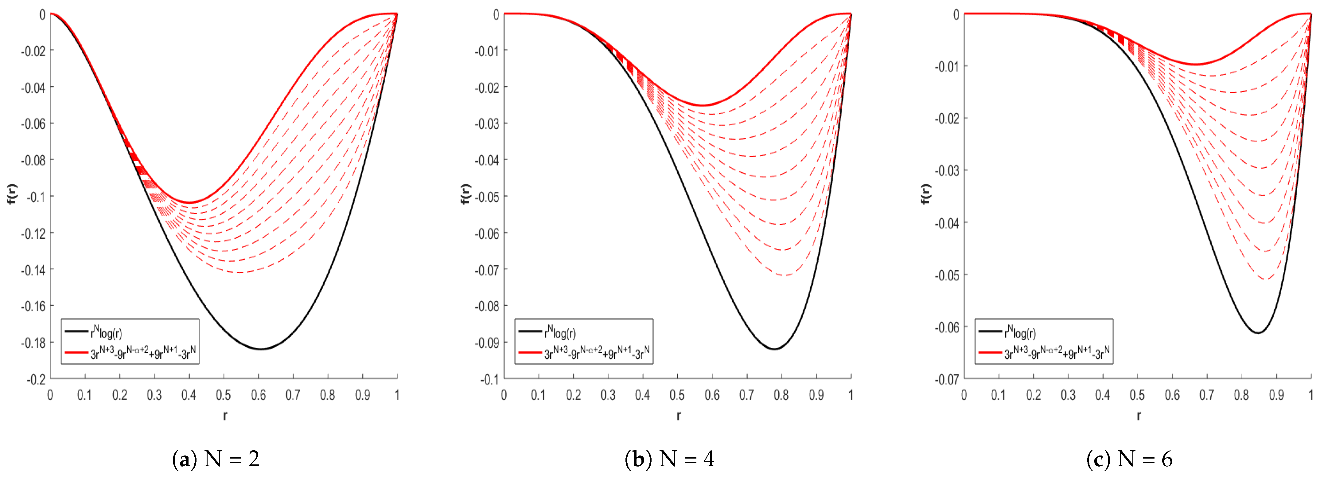
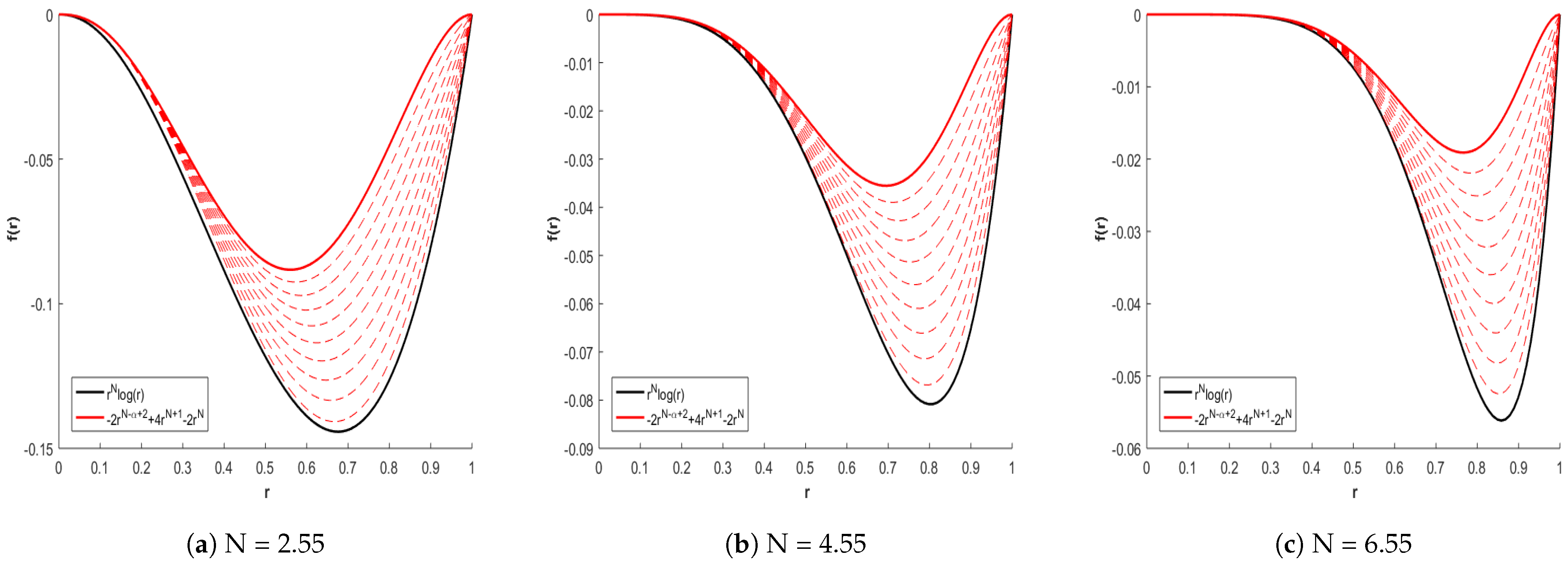
To enhance the previous approximation, a small perturbation α , where α [ 0 , 1 ) , is introduced in the exponent of the term with the highest power associated with a negative coefficient. Simultaneously, the exponent of this coefficient is adjusted by adding a perturbation + α . This leads to defining the following function:
Φ ( α , N , r ) = 3 b N r N + 3 9 b 1 N + α r N α + 2 + 9 b 2 N r N + 1 3 b 3 N r N ,
which in the domain Ω 1 fulfills the following (see Figure 6):
Φ ( α , N , r ) = 3 r N + 3 9 r N α + 2 + 9 r N + 1 3 r N r N log ( r ) .
On the other hand, it is worth mentioning that the construction of the polynomial (7) may be generalized by replacing the vector c with the following:
c = 0 c 0 ,
resulting in the following function:
Φ ( N , r ) = c 0 b N r N + 1 c 0 b 1 N r N .
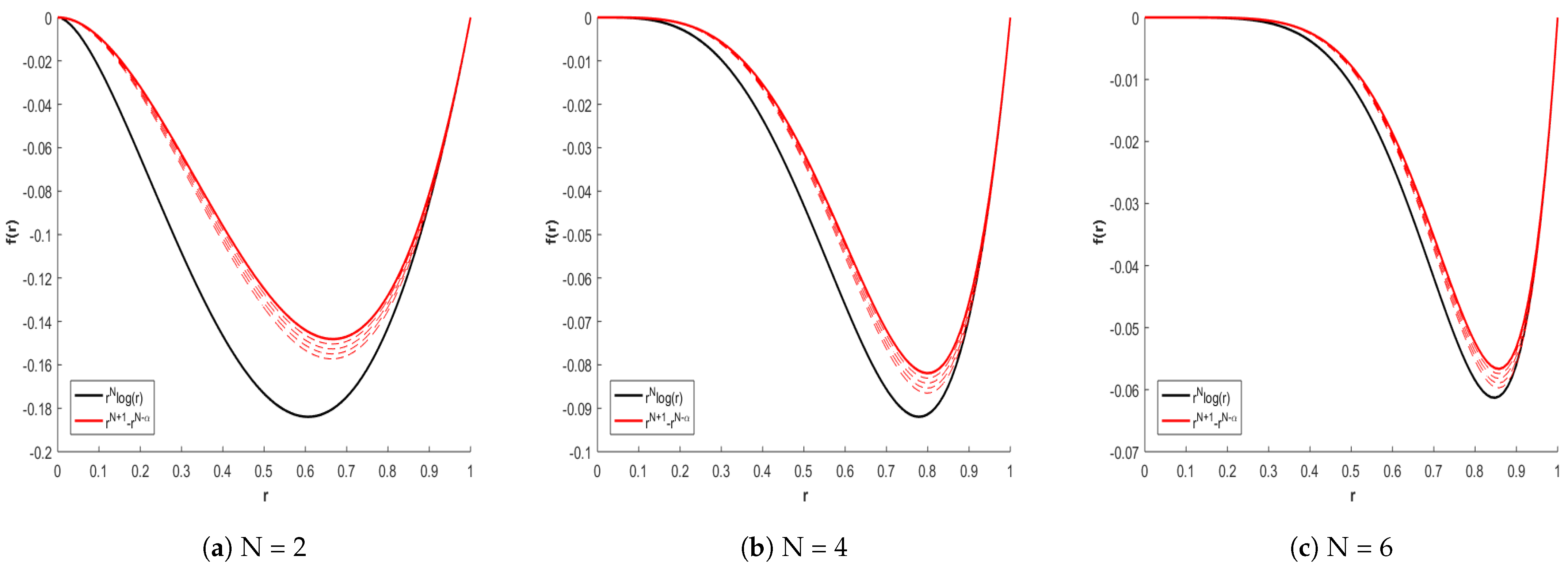
Taking the particular case c 0 = 1 , and to improve the previous approximation, a small perturbation α , where α [ 0 , 1 ) , is introduced in the exponent of the term with the highest power associated with a negative coefficient. Simultaneously, the exponent of this coefficient is adjusted by adding a perturbation + α . This leads to defining the following function:
Φ ( α , N , r ) = b N r N + 1 b 1 N + α r N α ,
which in the domain Ω 1 fulfills the following (see Figure 7):
Φ ( α , N , r ) = r N + 1 r N α r N log ( r ) .

2.3. Radial Functions with Behavior Similar to the TPS Function

The functions in Equations (22), (19), and (15) exhibit behavior similar to the TPS function within the domain Ω 1 . However, the objective is to obtain radial functions [10,11] that adhere to this behavior. To accomplish this, the following constraints are imposed:
N N   and   N α N ,
where N > 0 and α [ 0 , 1 ) . Henceforth, it will be assumed that all functions used implicitly adhere to the restrictions given in Equation (24), unless otherwise stated. By imposing the aforementioned constraints on polynomials (22), (15), and (19), this ensures obtaining radial functions that exhibit a behavior similar to the TPS function. To illustrate this, the pseudo TPS function is selected, and Equation (1) is allowed to take rational values, resulting in the graphs shown in Figure 8:

Conditionally Positive Definite Functions

In this section, a definition and a crucial theorem are introduced [11], which will be fundamental in the subsequent discussion.
Definition 1.
A function ϕ : [ 0 , ) R is said to be completely monotone  in [ 0 , ) if it belongs to C [ 0 , ) C ( 0 , ) and fulfills the following:
( 1 ) l ϕ ( l ) ( r ) 0 , r > 0 , l N .
Theorem 1.
(Michelli) Let ϕ C [ 0 , ) C ( 0 , ) be a given function. Then the function Φ = ϕ (   ·   2 ) is radial and conditionally positive definite of order m in R d for all d if and only if ( 1 ) m ϕ ( m ) is completely monotone in [ 0 , ) .
On the other hand, for future results, the following example is provided:
Example 1.
Let ϕ be a function defined as follows:
ϕ ( r ) = ( 1 ) β / 2 r β / 2 , 0 < β N ,
where r > 0 . Furthermore, the derivatives of the function ϕ are given by the following expressions:
ϕ ( 1 ) ( r ) = ( 1 ) β / 2 β 2 r ( β / 2 ) 1 , ϕ ( 2 ) ( r ) = ( 1 ) β / 2 β 2 β 2 1 r ( β / 2 ) 2 , ϕ ( l ) ( r ) = ( 1 ) β / 2 β 2 β 2 1 β 2 l + 1 r ( β / 2 ) l .
It should be noted that the last expression may be rewritten as follows:
ϕ ( l ) ( r ) = ( 1 ) β / 2 k = 1 l β 2 k + 1 r ( β / 2 ) l ,
with which it is possible to obtain the following result:
( 1 ) β / 2 ϕ ( β / 2 ) ( r ) = k = 1 β / 2 β 2 k + 1 r ( β / 2 ) β / 2 ,
and therefore, the following is fulfilled:
( 1 ) β / 2 ϕ ( β / 2 ) 0 1 β 2 k ,   k 1 β 2 β 2 β 2 β 2 + 1 ,
which means that ( 1 ) β / 2 ϕ ( β / 2 ) is completely monotonic. It is worth noting that m = β / 2 is the smallest value for which this is true. Since β is not a natural number, ϕ is not a polynomial. Therefore, the following functions
Φ ( x ) = ( 1 ) β / 2 x β , 0 < β N ,
are strictly conditionally positive definite of order β / 2 and radial in R d for all d.
A conditionally positive definite function of order m remains conditionally positive definite of order l m . Moreover, if a function is conditionally positive definite of order m in R d , then it is also conditionally positive definite of order m in R k for k d [10]. So, considering the previous example, it follows that the following function
Φ ( α , N , r ) = 2 r N α + 2 + 4 r N + 1 2 r N ,
is conditionally positive definite of order:
N α + 2 2 .

3. Interpolation with Radial Functions

Before proceeding, it is necessary to provide the following definition:
Definition 2.
Let Φ : R d R be a function. Then, Φ : R d R is called radial if there exists a function ϕ : R 0 R such that
Φ ( x ) = ϕ ( x ) ,
where   ·   : R d R denotes any vector norm (generally the Euclidean norm).
Given a set of values ( x j , u j ) j = 1 N p , where ( x j , u j ) Ω × R with Ω R d , an interpolant is a function σ : Ω R that fulfills the following:
σ ( x j ) = u j , j 1 , , N p .
On the other hand, let P m 1 ( R d ) be the space of polynomials in d variables of degree less than m. So, when using a conditionally positive definite radial function Φ , it is possible to propose an interpolant of the following form [10,11]:
σ ( x ) = j = 1 N p λ j Φ ( x x j ) + k = 1 Q β k p k ( x ) ,
where Q = dim ( P m 1 ( R d ) ) and p k k = 1 Q forms a basis for P m 1 ( R d ) . Additionally, it is worth mentioning that the interpolation conditions given in Equation (26) are complemented by the following moment conditions:
j = 1 N p λ j p k ( x j ) = 0 , k 1 , , Q .
Before continuing, it should be noted that solving the interpolation problem given in Equation (26) using the interpolant (27), along with the moment conditions (28), is equivalent to solving the following linear system:
A P P T 0 G λ β Λ = u 0 U ,
where A and P are matrices of dimensions ( N p × N p ) and ( N p × Q ) respectively, with the components
A j k = Φ ( x j x k ) , P j k = p k ( x j ) .
The condition that a function Φ is conditionally positive definite of order m may ensure that the matrix A with components A j k = Φ ( x j x k ) is positive definite in the space of vectors c R N p , such that
j = 1 N p c j p k ( x j ) = 0 , k 1 , , Q .
As a consequence, if in Equation (27) the function Φ is conditionally positive definite of order m and the set of centers x j j = 1 N p contains a unisolvent subset, the interpolation problem will have a unique solution [10,11].

Examples with Radial Functions

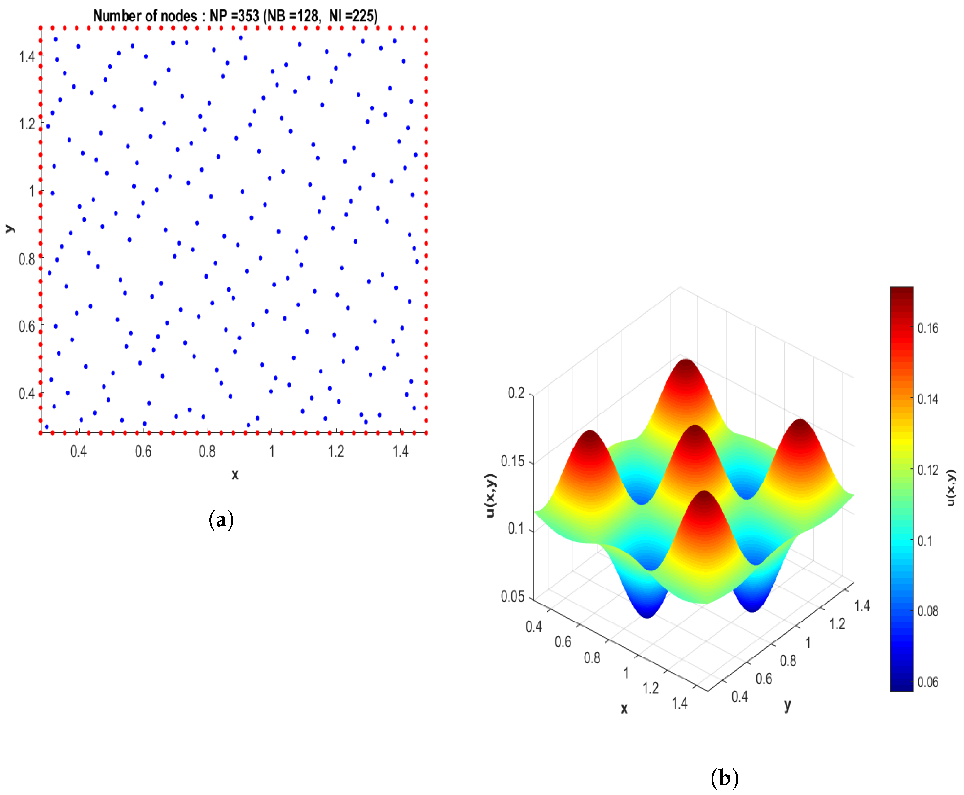
Before proceeding, it is necessary to define the following domain for the subsequent examples:
Ω a , b : = [ a , b ] × [ a , b ] .
So, considering the following function:
u ( x , y ) = sin ( 8 ( x + y ) ) + cos ( 8 ( x y ) ) + 4 35 ,
and considering a distribution of nodes in a Halton-type pattern over the domain Ω 0.28 , 1.48 , it is possible to visualize a graph of the function above (see Figure 9).
Thus, to perform the interpolation examples, a set of values u ( x i , y i ) i = 1 N p Ω 0.28 , 1.48 are generated, along with a sequence of values α i i = 1 N α [ 0 , 1 ) . So, denoting σ i = σ ( x i , y i ) and u i = u ( x i , y i ) , it is possible to use the root mean square error (RMSE) to get an idea of the error generated in the interpolation problems, which is defined as follows:
R M S E : = 1 N p i = 1 N p u i σ i 2 .
Additionally, for the following examples, the condition number of the matrix G from Equation (29) is defined as follows:
c o n d ( G ) = G · G 1 ,
where G 1 denotes any matrix norm of the inverse matrix of G (generally the Euclidean norm).
Example 2.
Using the generalized pseudo TPS function
Φ ( α , N , r ) = 2 b N + α r N α + 2 + 4 b 1 N r N + 1 2 b 2 N r N ,
with N = 3.22 . Then, to use the interpolant (27) considering the previous function, the value of m that allows defining the value of Q may be assigned by considering the endpoints of the interval, where the values α i are taken as follows:
m = max N 0 + 2 2 , N 1 + 2 2 = 3 ,
with which the results shown in Table 1 are obtained.
Example 3.
Using the radial function
Φ ( α , N , r ) = 3 b N r N + 3 9 b 1 N + α r N α + 2 + 9 b 2 N r N + 1 3 b 3 N r N ,
with N = 2.55 . Then, to use the interpolant (27) considering the previous function, the value of m that allows defining the value of Q may be assigned as follows:
m = N + 3 2 = 3 ,
with which the results shown in Table 2 are obtained.
To conclude this section, it is worth noting that in the previous examples, the condition number of the obtained matrices was excessively high. Therefore, before proceeding, a method is proposed to reduce the condition number of these matrices. For this purpose, the linear system (29) may be written in a compact form as follows:
G Λ = U ,
where G is a matrix of size ( N p + Q ) × ( N p + Q ) , and Λ and U are column vectors of size ( N p + Q ) . So, to address the issue of reducing the condition number of the previous system, the Q R decomposition of the matrix G is employed [36]; that is,
G = Q R ,
with which it is feasible to replace the linear system (29) with the following equivalent system:
G M Λ = H R 1 G Λ = ( H R ) 1 U = U M ,
where the matrix H is defined by the following components:
H i j = Q i j + 1 2 n , n N ,
in which the value of n is chosen based on the following conditions:
c o n d G M M c o n d ( G ) .
Before proceeding, it is important to clarify that in the upcoming examples, the preconditioned linear system (34) will be used considering the value M = 10 .

4. Fractional Operators

Fractional calculus is a branch of mathematics that involves derivatives of non-integer order, and it emerged around the same time as conventional calculus, in part due to Leibniz’s notation for derivatives of integer order:
d n d x n .
Thanks to this notation, L’Hopital was able to inquire in a letter to Leibniz about the interpretation of taking n = 1 / 2 in a derivative. At that moment, Leibniz could not provide a physical or geometrical interpretation for this question, so he simply replied to L’Hopital in a letter that “… is an apparent paradox from which, one day, useful consequences will be drawn” [37]. The name “fractional calculus” comes from a historical question, as in this branch of mathematical analysis, derivatives and integrals of a certain order α are studied, with α R . Currently, fractional calculus does not have a unified definition of what is considered a fractional derivative. As a consequence, when it is not necessary to explicitly specify the form of a fractional derivative, it is usually denoted as follows:
d α d x α .
Fractional operators have various representations, but one of their fundamental properties is that they recover the results of conventional calculus when α n . Before continuing, it is worth mentioning that due to the large number of fractional operators that exist [38,39,40,41,42,43,44,45,46,47,48,49,50,51,52,53,54,55,56], it seems that the most natural way to fully characterize the elements of fractional calculus is by using sets, which is the main idea behind the methodology known as fractional calculus of sets [57,58,59,60], whose seed of origin is the fractional Newton–Raphson method [24]. Therefore, considering a scalar function h : R m R and the canonical basis of R m denoted by e ^ k k 1 , it is feasible to define the following fractional operator of order α using Einstein’s notation:
o x α h ( x ) : = e ^ k o k α h ( x ) .
Therefore, denoting k n as the partial derivative of order n applied with respect to the k-th component of the vector x, using the previous operator, it is feasible to define the following set of fractional operators:
O x , α n ( h ) : = o x α   :   o k α h ( x )   and   lim α n o k α h ( x ) = k n h ( x )   k 1 ,
which corresponds to a nonempty set since it contains the following sets of fractional operators:
O 0 , x , α n ( h ) : = o x α   :   o k α h ( x ) = k n + μ ( α ) k α h ( x )   and   lim α n μ ( α ) k α h ( x ) = 0   k 1 .
As a consequence, the following result may be obtained:
If   o i , x α , o j , x α O x , α n ( h )   with   i j     o k , x α = 1 2 o i , x α + o j , x α O x , α n ( h ) .
On the other hand, the complement of the set (36) may be defined as follows:
O x , α n , c ( h ) : = o x α   :   o k α h ( x )   k 1   and   lim α n o k α h ( x ) k n h ( x )   in at least one value k 1 ,
with which it is feasible to obtain the following result:
If   o i , x α = e ^ k o i , k α O x , α n ( h )     o j , x α = e ^ k o i , σ j ( k ) α O x , α n , c ( h ) ,
where σ j : 1 , 2 , , m 1 , 2 , , m denotes any permutation different from the identity. On the other hand, considering a function h : Ω R m R m , it is feasible to define the following sets:
m O x , α n ( h ) : = o x α   :   o x α O x , α n [ h ] k   k m ,  
m O x , α n , c ( h ) : = o x α   :   o x α O x , α n , c [ h ] k   k m ,  
m O x , α n , u ( h ) : = m O x , α n ( h ) m O x , α n , c ( h ) ,
where [ h ] k : Ω R m R denotes the k-th component of the function h. So, the following set of fractional operators may be defined:
m MO x , α , u ( h ) : = k Z m O x , α k , u ( h ) ,
which under the classical Hadamard product fulfills that
o x 0 h ( x ) : = h ( x )   o x α   m MO x , α , u ( h ) .
Furthermore, it is worth noting that for each operator o x α m MO x , α , u ( h ) , it is feasible to define the following fractional matrix operator:
A α o x α = [ A α o x α ] j k : = o k α .
On the other hand, considering that when using the classical Hadamard product, in general o x p α o x q α o x ( p + q ) α , it is feasible to define the following modified Hadamard product [57,60]:
o i , x p α o j , x q α : = o i , x p α o j , x q α , if i j   ( Hadamard product of type horizontal )   o i , x ( p + q ) α , if i = j   ( Hadamard product of type vertical ) ,
with which for each operator o x α m MO x , α , u ( h ) , a group isomorphic to the group of integers under the addition may be defined, which corresponds to the abelian group generated by the operator A α o x α , denoted as follows: [58,61]:
m G A α o x α : = A α r = A α o x r α   :   r Z   and   A α r = [ A α r ] j k : = o k r α .
Before proceeding, it is worth mentioning that some applications may be derived based on the previous definition, among which the following corollary can be found [59,60]:
Corollary 1.
Let o x α be a fractional operator such that o x α m MO x , α , u ( h ) and let Z , + be the group of integers under the addition. Therefore, considering the modified Hadamard product given by (47) and some subgroup H of the group Z , + , it is feasible to define the following set of fractional matrix operators:
m G A α o x α , H : = A α r = A α o x r α   :   r H   a n d   A α r = [ A α r ] j k : = o k r α ,
which corresponds to a subgroup of the group generated by the operator A α o x α ; that is,
m G A α o x α , H m G A α o x α .
Example 4.
Let Z n be the set of residual classes less than a positive integer n. Therefore, considering a fractional operator o x α m MO x , α , u ( h ) and the set Z 14 , it is feasible to define, under the modified Hadamard product given by (47), the following abelian group of fractional matrix operators:
m G A α o x α , Z 14 = A α 0 , A α 1 , A α 2 , A α 3 , A α 4 , A α 5 , A α 6 , A α 7 , A α 8 , A α 9 , A α 10 , A α 11 , A α 12 , A α 13 .
Furthermore, all possible combinations of the elements of the group are summarized in the following Cayley table:
A α 0 A α 1 A α 2 A α 3 A α 4 A α 5 A α 6 A α 7 A α 8 A α 9 A α 10 A α 11 A α 12 A α 13 A α 0 A α 0 A α 1 A α 2 A α 3 A α 4 A α 5 A α 6 A α 7 A α 8 A α 9 A α 10 A α 11 A α 12 A α 13 A α 1 A α 1 A α 2 A α 3 A α 4 A α 5 A α 6 A α 7 A α 8 A α 9 A α 10 A α 11 A α 12 A α 13 A α 0 A α 2 A α 2 A α 3 A α 4 A α 5 A α 6 A α 7 A α 8 A α 9 A α 10 A α 11 A α 12 A α 13 A α 0 A α 1 A α 3 A α 3 A α 4 A α 5 A α 6 A α 7 A α 8 A α 9 A α 10 A α 11 A α 12 A α 13 A α 0 A α 1 A α 2 A α 4 A α 4 A α 5 A α 6 A α 7 A α 8 A α 9 A α 10 A α 11 A α 12 A α 13 A α 0 A α 1 A α 2 A α 3 A α 5 A α 5 A α 6 A α 7 A α 8 A α 9 A α 10 A α 11 A α 12 A α 13 A α 0 A α 1 A α 2 A α 3 A α 4 A α 6 A α 6 A α 7 A α 8 A α 9 A α 10 A α 11 A α 12 A α 13 A α 0 A α 1 A α 2 A α 3 A α 4 A α 5 A α 7 A α 7 A α 8 A α 9 A α 10 A α 11 A α 12 A α 13 A α 0 A α 1 A α 2 A α 3 A α 4 A α 5 A α 6 A α 8 A α 8 A α 9 A α 10 A α 11 A α 12 A α 13 A α 0 A α 1 A α 2 A α 3 A α 4 A α 5 A α 6 A α 7 A α 9 A α 9 A α 10 A α 11 A α 12 A α 13 A α 0 A α 1 A α 2 A α 3 A α 4 A α 5 A α 6 A α 7 A α 8 A α 10 A α 10 A α 11 A α 12 A α 13 A α 0 A α 1 A α 2 A α 3 A α 4 A α 5 A α 6 A α 7 A α 8 A α 9 A α 11 A α 11 A α 12 A α 13 A α 0 A α 1 A α 2 A α 3 A α 4 A α 5 A α 6 A α 7 A α 8 A α 9 A α 10 A α 12 A α 12 A α 13 A α 0 A α 1 A α 2 A α 3 A α 4 A α 5 A α 6 A α 7 A α 8 A α 9 A α 10 A α 11 A α 13 A α 13 A α 0 A α 1 A α 2 A α 3 A α 4 A α 5 A α 6 A α 7 A α 8 A α 9 A α 10 A α 11 A α 12
On the other hand, it is important to highlight that Corollary 1 allows generating groups of fractional operators under other operations [59]. For example, considering the following operation
A α r A α s = A α r s ,
it is feasible to obtain the following corollary:
Corollary 2.
Let Z p + be the set of positive residual classes less than p, with p a prime number. Therefore, for each fractional operator o x α m MO x , α , u ( h ) , it is feasible to define the following abelian group of fractional matrix operators under the operation (52):
m G * A α o x α , Z p + : = A α r = A α o x r α   :   r Z p +   a n d   A α r = [ A α r ] j k : = o k r α .
Example 5.
Let o x α be a fractional operator such that o x α m MO x , α , u ( h ) . Therefore, considering the set Z 13 + , it is feasible to define, under the operation (52), the following abelian group of fractional matrix operators:
m G * A α o x α , Z 13 + = A α 1 , A α 2 , A α 3 , A α 4 , A α 5 , A α 6 , A α 7 , A α 8 , A α 9 , A α 10 , A α 11 , A α 12 .
Furthermore, all possible combinations of the elements of the group are summarized in the following Cayley table:
A α 1 A α 2 A α 3 A α 4 A α 5 A α 6 A α 7 A α 8 A α 9 A α 10 A α 11 A α 12 A α 1 A α 1 A α 2 A α 3 A α 4 A α 5 A α 6 A α 7 A α 8 A α 9 A α 10 A α 11 A α 12 A α 2 A α 2 A α 4 A α 6 A α 8 A α 10 A α 12 A α 1 A α 3 A α 5 A α 7 A α 9 A α 11 A α 3 A α 3 A α 6 A α 9 A α 12 A α 2 A α 5 A α 8 A α 11 A α 1 A α 4 A α 7 A α 10 A α 4 A α 4 A α 8 A α 12 A α 3 A α 7 A α 11 A α 2 A α 6 A α 10 A α 1 A α 5 A α 9 A α 5 A α 5 A α 10 A α 2 A α 7 A α 12 A α 4 A α 9 A α 1 A α 6 A α 11 A α 3 A α 8 A α 6 A α 6 A α 12 A α 5 A α 11 A α 4 A α 10 A α 3 A α 9 A α 2 A α 8 A α 1 A α 7 A α 7 A α 7 A α 1 A α 8 A α 2 A α 9 A α 3 A α 10 A α 4 A α 11 A α 5 A α 12 A α 6 A α 8 A α 8 A α 3 A α 11 A α 6 A α 1 A α 9 A α 4 A α 12 A α 7 A α 2 A α 10 A α 5 A α 9 A α 9 A α 5 A α 1 A α 10 A α 6 A α 2 A α 11 A α 7 A α 3 A α 12 A α 8 A α 4 A α 10 A α 10 A α 7 A α 4 A α 1 A α 11 A α 8 A α 5 A α 2 A α 12 A α 9 A α 6 A α 3 A α 11 A α 11 A α 9 A α 7 A α 5 A α 3 A α 1 A α 12 A α 10 A α 8 A α 6 A α 4 A α 2 A α 12 A α 12 A α 11 A α 10 A α 9 A α 8 A α 7 A α 6 A α 5 A α 4 A α 3 A α 2 A α 1
Before proceeding, it is worth mentioning that while the above theory may seem overly abstract and restrictive at first, when considering specific cases, the results may be applied to a wide variety of well-known fractional operators in the literature. Among this is the operator Riemann–Liouville fractional integral, defined as follows [35,62]:
a I x α f ( x ) : = 1 Γ α a x ( x t ) α 1 f ( t ) d t ,
which allows constructing the operator Riemann–Liouville fractional derivative, defined as follows [62,63]:
a D x α f ( x ) : = a I x α f ( x ) , if α < 0   d n d x n a I x n α f ( x ) , if α 0 ,
where n = α and a I x 0 f ( x ) : = f ( x ) . Furthermore, operator (55) also enables the construction the operator Caputo fractional derivative, defined as follows [62,63]:
a C D x α f ( x ) : = a I x α f ( x ) , if α < 0   a I x n α f ( n ) ( x ) , if α 0 ,
where n = α and a I x 0 f ( n ) ( x ) : = f ( n ) ( x ) . So, to exemplify the aforementioned point that in specific cases the previous theory may be extended to multiple fractional operators, considering α [ 0 , 1 ) , for the specific value α = 1 / 14 , it is feasible to replicate the results from Example 4 with the fractional operators (55)–(57), individually or in any combination when constructing a fractional operator using the definition (43). Similarly, for the specific value α = 1 / 13 , the results from Example 5 may be replicated with the aforementioned fractional operators. This opens the possibility of obtaining applications different from the conventional ones for fractional operators, since they are commonly used in the literature to replace derivatives and integrals of integer order in models aimed at predicting the behavior of certain physical phenomena, to achieve greater accuracy.
On the other hand, it is important to mention that if a function f fulfills the condition f ( k ) ( a ) = 0   k 0 , 1 , , n 1 , the Riemann–Liouville fractional derivative coincides with the Caputo fractional derivative; that is,
a D x α f ( x ) = a C D x α f ( x ) .
So, applying operator (56) with a = 0 to the function x μ , with μ > 1 , the following result is obtained: [26]:
0 D x α x μ = Γ μ + 1 Γ μ α + 1 x μ α , α R Z ,
where if 1 α μ , it is fulfilled that 0 D x α x μ = 0 C D x α x μ . On the other hand, it is worth noting that, as shown in the above equation, the perturbations α used in the functions that may be extended from the pseudo TPS function given in Equations (15) and (19) bear a certain resemblance to the application of fractional operators (56) and (57) to functions of the form r N + 2 . Thus, proposing another application of fractional operators different from the conventional, in Equations (15) and (19), it is feasible to carry out the following substitution:
r N α + 2 0 D r α r N + 2 ,
resulting in the following modified functions:
Φ ( α , N , r ) = 2 b N + α 0 D r α r N + 2 + 4 b 1 N r N + 1 2 b 2 N r N ,
Φ ( α , N , r ) = 3 b N r N + 3 9 b 1 N + α 0 D r α r N + 2 + 9 b 2 N r N + 1 3 b 3 N r N .

4.1. Examples with Partially Implemented Fractional Derivative

In the upcoming examples, Equation (32) will be employed once more, in conjunction with the node distribution illustrated in Figure 9, and the set of values u i i = 1 N p are generated accordingly. Additionally, the fractional derivative, defined in Equation (59) with α ( 1 , 1 ) , will be applied. So, the results presented below are obtained:
Example 6.
Using the modified function (60) with N = 3.22 . Then, to use the interpolant (27) considering the previous function, the value of m that allows defining the value of Q may be assigned by considering the endpoints of the interval where the values α i are taken as follows:
m = max N ( 1 ) + 2 2 , N 1 + 2 2 = 4 ,
with which the results shown in Table 3 are obtained.
Example 7.
Using the modified function (61) with N = 2.55 . Then, to use the interpolant (27) considering the previous function, the value of m that allows defining the value of Q may be assigned as follows:
m = N + 3 2 = 3 ,
with which the results shown in Table 4 are obtained.

4.2. Examples with Fully Implemented Fractional Derivative

Considering that the partial implementation of fractional derivatives in the functions from the previous examples resulted in well-behaved errors, the next step is to fully implement fractional derivatives in the functions (15) and (19) to analyze the behavior of the errors. This is accomplished through the following substitution:
b s r t b s + α 0 D r α r t ,
resulting in the following modified functions:
Φ ( α , N , r ) = 2 b N + α 0 D r α r N + 2 + 4 b 1 N + α 0 D r α r N + 1 2 b 2 N + α 0 D r α r N ,
Φ ( α , N , r ) = 3 b N + α 0 D r α r N + 3 9 b 1 N + α 0 D r α r N + 2 + 9 b 2 N + α 0 D r α r N + 1 3 b 3 N + α 0 D r α r N .
Then, applying the fractional derivative defined in Equation (59) with α ( 1 , 1 ) , the results presented below are obtained:
Example 8.
Using the modified function (62) with N = 3.22 . Then, to use the interpolant (27) considering the previous function, the value of m that allows defining the value of Q may be assigned by considering the endpoints of the interval where the values α i are taken as follows:
m = max N ( 1 ) + 2 2 , N 1 + 2 2 = 4 ,
with which the results shown in Table 5 are obtained.
Example 9.
Using the modified function (63) with N = 2.55 . Then, to use the interpolant (27) considering the previous function, the value of m that allows defining the value of Q may be assigned as follows:
m = N + 3 2 = 3 ,
with which the results shown in Table 6 are obtained.

A Change in the Interpolant

In the preceding sections, the interpolator given by Equation (27) was utilized, where Q = dim P m 1 R d . This leads to a substantial increase in the value of Q for certain cases. For instance, considering a polynomial in R 2 of degree 4, results in Q being equal to 15. Recognizing that sometimes simplicity is key to solving certain problems, it is proposed to modify the polynomial in the interpolator (27) with a radial polynomial, such that Q = dim P m 1 R . This allows the proposal of the following interpolant:
σ ( x ) = j = 1 N p λ j Φ ( x x j ) + k = 0 Q β k r k ( x ) .
As a consequence, the moment conditions may be rewritten as follows:
j = 1 N p λ j r k = 0 , k 0 , 1 , , Q .
With the previous changes, the advantage is gained that, when considering a radial polynomial in R of degree 4, the value of Q would be equal to 5. Then, the following examples are presented using the modified interpolant (64):
Example 10.
Using the modified function (62) with N = 3.22 . Then, to use the interpolant (27) considering the previous function, the value of m that allows defining the value of Q may be assigned by considering the endpoints of the interval where the values α i are taken as follows:
m = max N ( 1 ) + 2 2 , N 1 + 2 2 = 4 ,
with which the results shown in Table 7 are obtained.
Example 11.
Using the modified function (61) with N = 2.55 . Then, to use the interpolant (27) considering the previous function, the value of m that allows defining the value of Q may be assigned as follows:
m = N + 3 2 = 3 ,
with which the results shown in Table 8 are obtained.

5. Asymmetrical Collocation

Before commencing this section, it is crucial to note that the interpolation technique discussed earlier may also be extended to solve differential equations [10]. So, considering a domain Ω R d and the following problem
L u = f , Ω , B u = g , Ω ,
where f and g are given functions, L and B are linear differential operators, and u is the sought solution. Before proceeding, a modification to the interpolant (64) is necessary, to avoid discontinuities caused by the application of the operators L and B . Denoting by o r d ( · ) the order of the differential operators, it is feasible to define the following values:
q = max o r d ( L ) , o r d ( B )   ,
o = q 1 , if q > 0 , 0 , if q 0 .
Then, the interpolant (64) may be rewritten as follows:
σ ( x ) = j = 1 N p λ j Φ ( x x j ) + β 0 + k = 1 Q β k r k + o ( x ) ,
where Q = dim P m 1 R . As a consequence, the moment conditions take the form:
j = 1 N p λ j p 1 = j = 1 N p λ j = 0 , j = 1 N p λ j p k + 1 = j = 1 N p λ j r k + o = 0 , k 1 , , Q .
In addition to the constraints given in (24), it is necessary to add the following restriction:
N > q + α , if q > 0 , N > α , if q 0 .
On the other hand, when substituting the interpolant (69) as a potential solution of the system (66); that is,
L σ = f , Ω , B σ = g , Ω ,
the following linear system is obtained:
L A L P B A B P P T 0 G λ β Λ = f g 0 U ,
where L A , B A , L P , B P , and P are matrices of dimensions ( N I × N p ) , ( ( N p N I ) × N p ) , ( N I × Q ) , ( ( N p N I ) × Q ) , and ( N p × Q ) respectively, whose components are given by the following expressions:
L A j k = L Φ ( x j x k ) , L P j k = L p k ( x j ) , B A j k = B Φ ( x j x k ) , B P j k = B p k ( x j ) , P j k = p k ( x j ) .

Examples with Fractional Differential Operators

Before proceeding, it should be noted that the interpolant provided by Equation (69) features a structure that is particularly effective for solving radial differential equations, which will be the main focus in the following examples. Furthermore, by utilizing the Caputo fractional derivative (57), it is feasible to construct the following fractional radial differential operator [31]:
L : = 0 C D r 2 + β + 1 r 0 C D r 1 + β + β r ,
and considering the operator B as the identity operator, the following differential equation may be formulated:
L u = f , Ω , u = g , Ω ,
which has the special feature that when β 0 , it takes the form of Poisson’s equation; that is,
2 u = f , Ω , u = g , Ω .
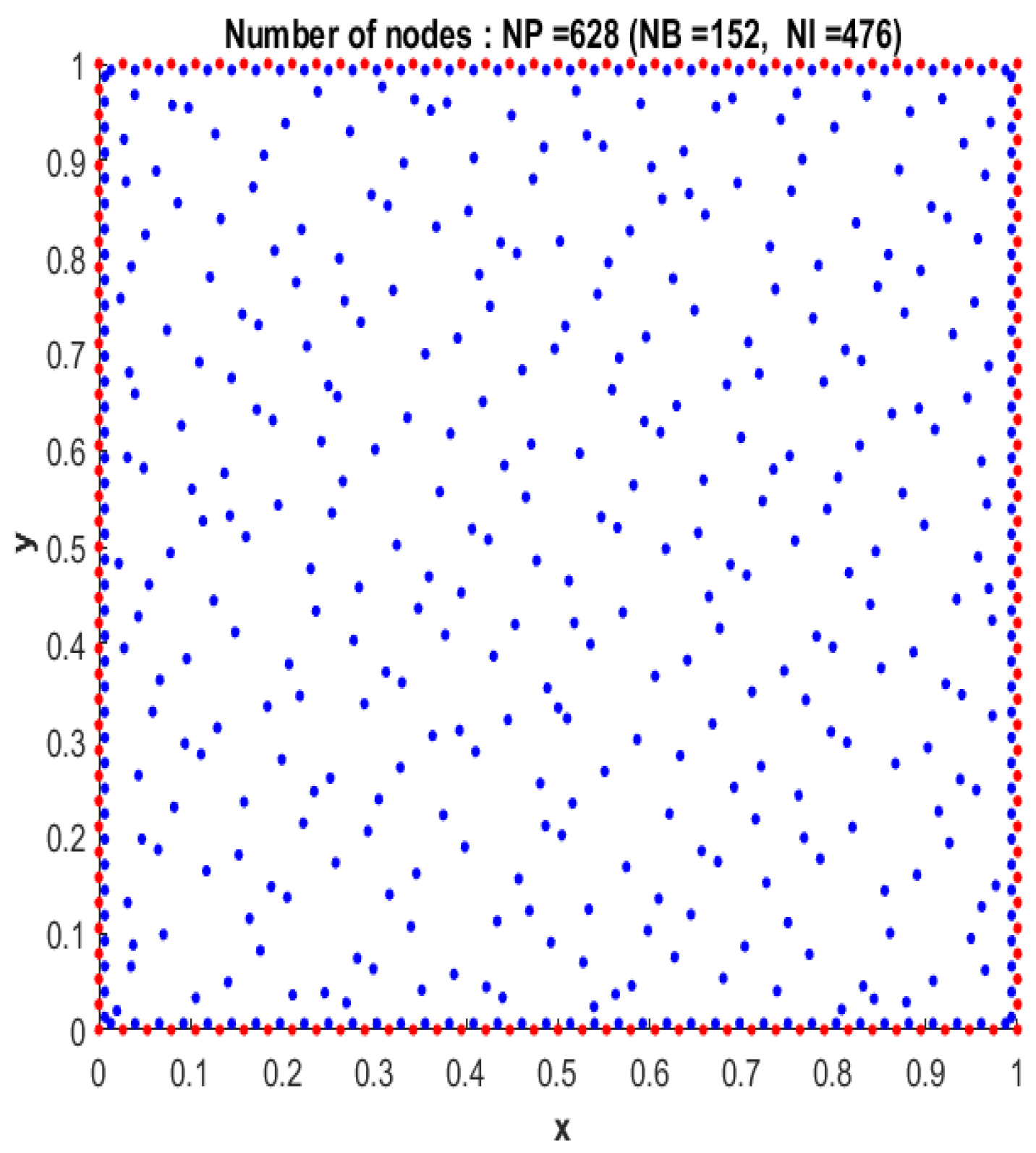
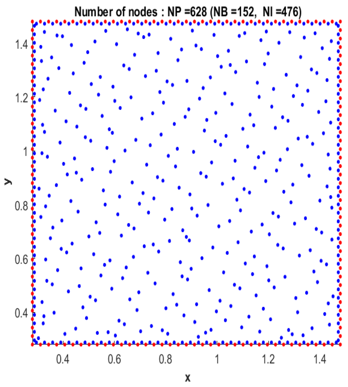
So, to solve the system (74) in the following examples, a distribution of interior nodes based on Halton-type nodes combined with Cartesian nodes near the boundary of the domain Ω 0 , 1 is considered, as shown in Figure 10, along with a sequence of values α i i = 1 N α ( 2 , 2 ) . Furthermore, denoting L σ i = L σ ( x i , y i ) and f i = f ( x i , y i ) , the mean square error from Equation (33) may be written as follows:
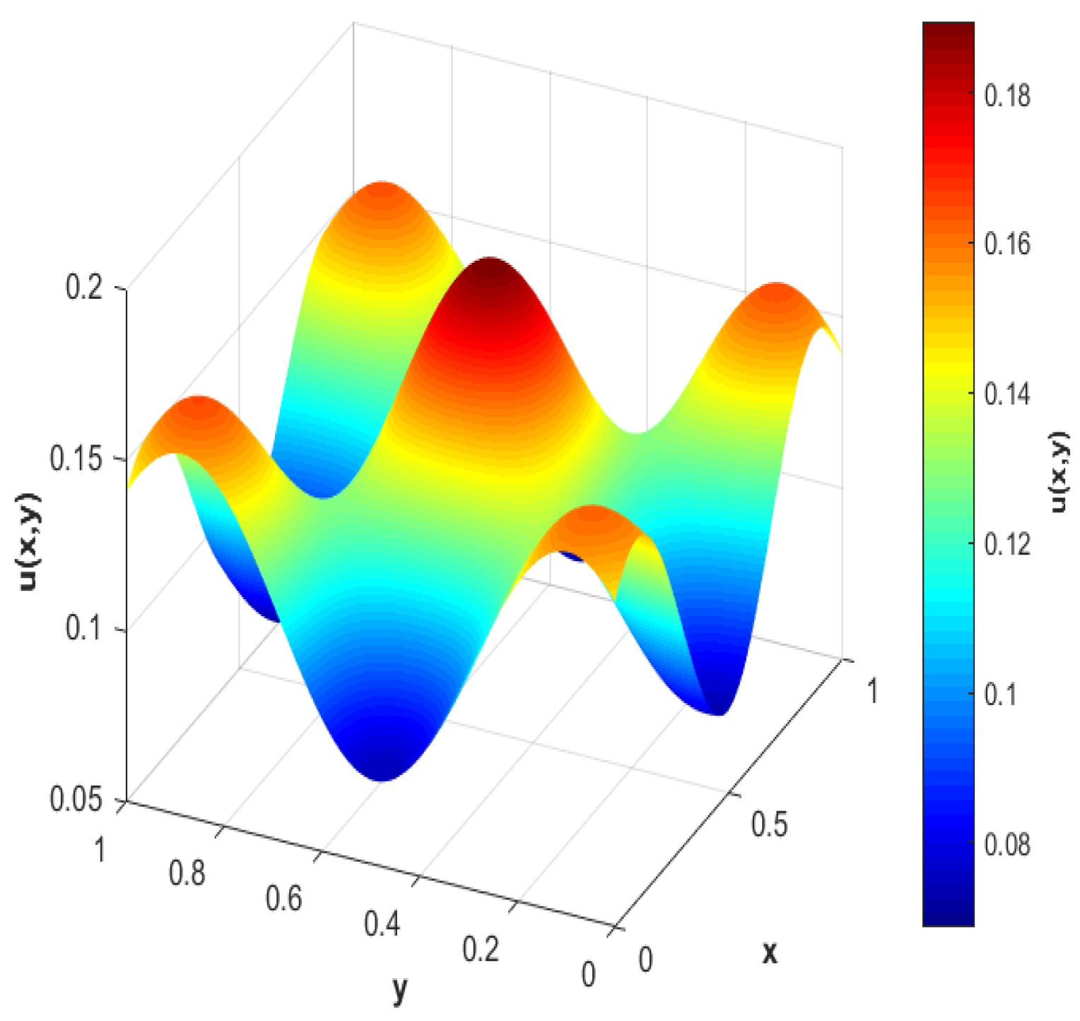
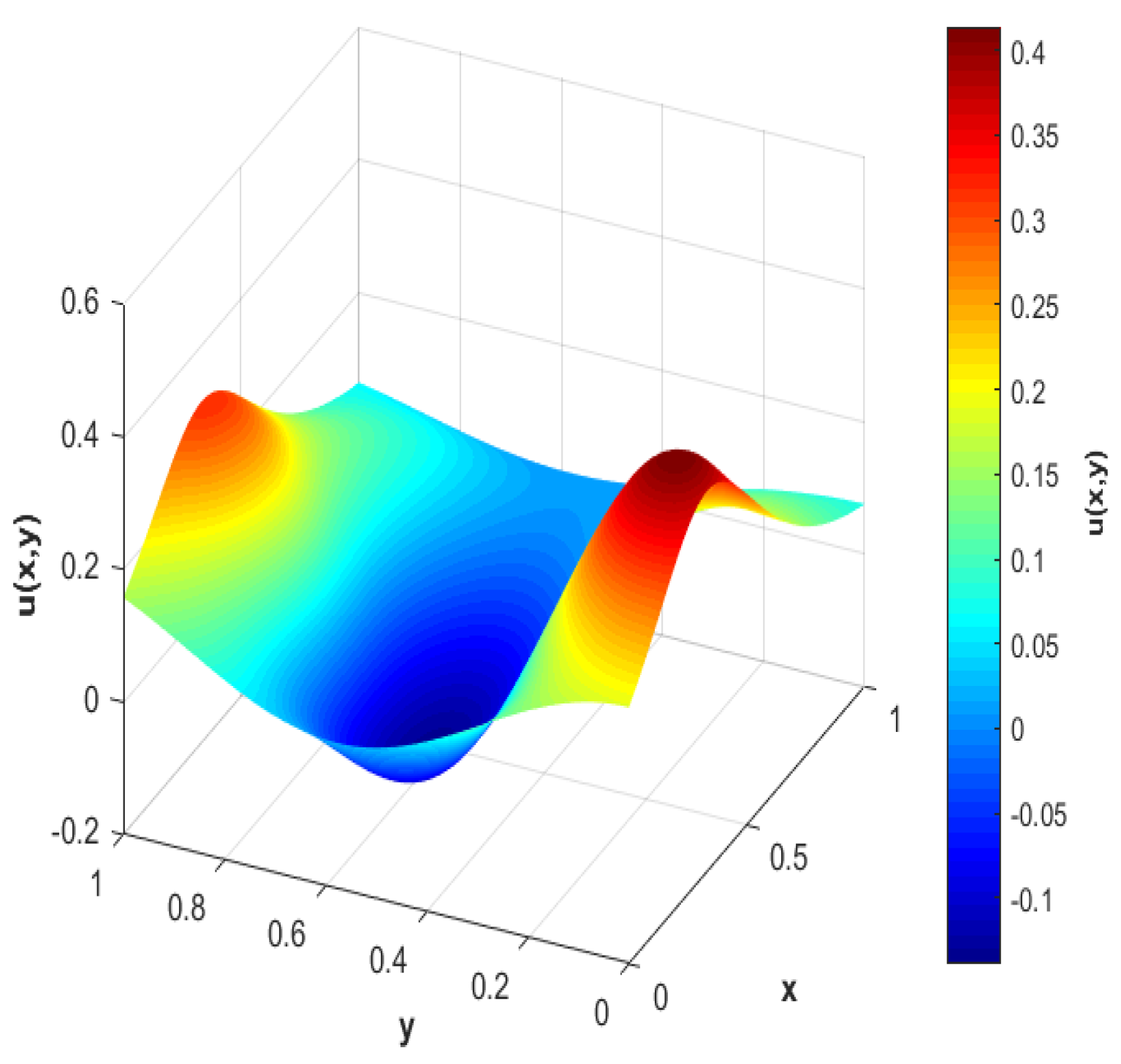
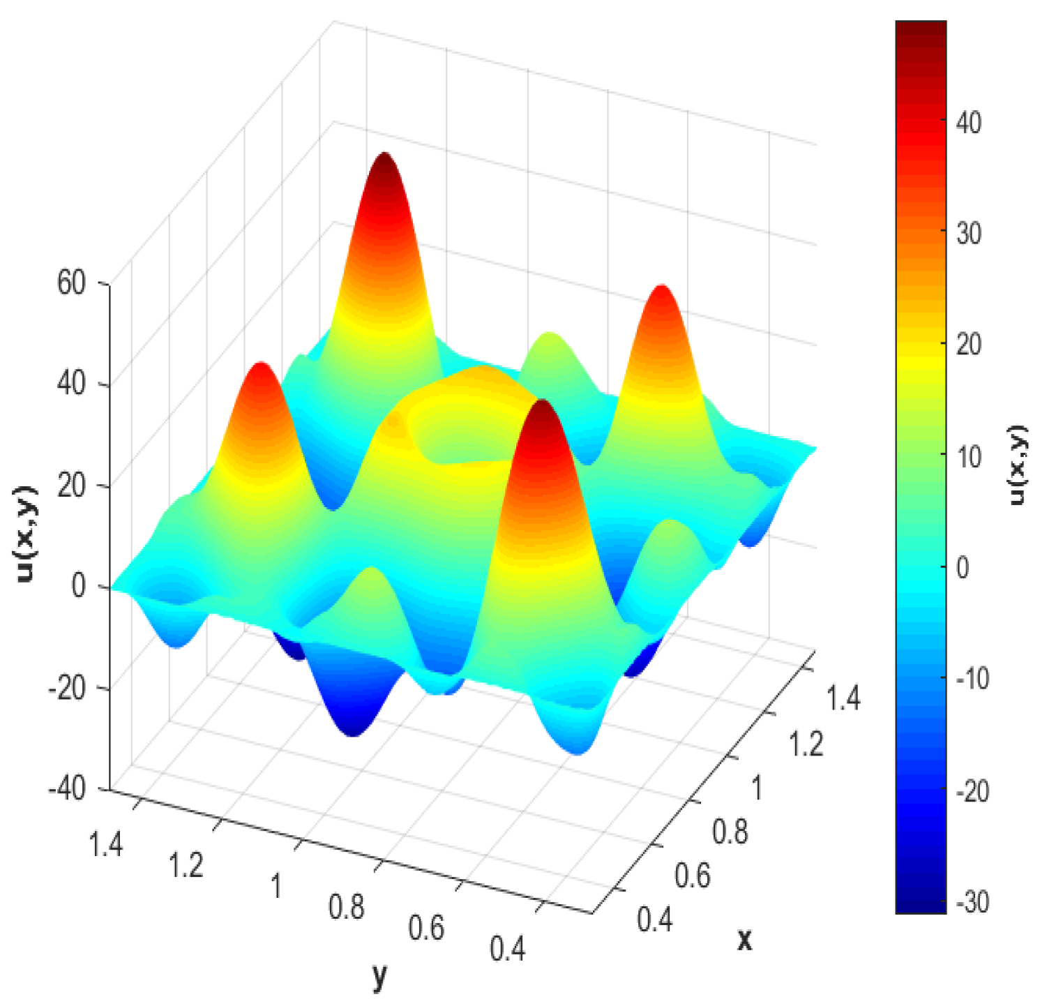
R M S E : = 1 N p i = 1 N p f i L σ i 2 .
Example 12.
Considering the value β = 0.5 in the differential operator (73) and the following functions in the system (74):
f ( x , y ) = 2 ( 108 x 36 ) 2 ( cos ( 5.4 y ) + 1.25 ) ( 6 ( 3 x 1 ) 2 + 6 ) 3 108 cos ( 5.4 y ) + 135 ( 6 ( 3 x 1 ) 2 + 6 ) 2 29.16 cos ( 5.4 y ) 6 ( 3 x 1 ) 2 + 6 , g ( x , y ) = cos ( 5.4 y ) + 1.25 6 ( 3 x 1 ) 2 + 6 .
So, to use the interpolant (69), the following values are calculated:
q = max 2 + β , 0 = 1.5 , o = q 1 = 0.5 ,
along with the values of N and m (since the latter allows defining the value of Q), which may be assigned by considering the endpoints of the interval where the values α i are taken, as follows:
max q + ( 2 ) , q + 2 = 3.5 < N = 3.55 ,
m = max N ( 2 ) + 2 2 , N 2 + 2 2 = 4 .
Finally, using the modified function (62) with the previous value of N in the interpolant, the results shown in Table 9 are obtained, and the graph of the numerical solution of the system with the minimal error obtained is shown in Figure 11.
Example 13.
Considering the value β = 0.15 in the differential operator (73) and the following functions in the system (74):
f ( x , y ) = 128 35 sin ( 8 ( x + y ) ) + cos ( 8 ( x y ) ) , g ( x , y ) = 1 35 sin ( 8 ( x + y ) ) + cos ( 8 ( x y ) ) + 4 .
So, to use the interpolant (69), the following values are calculated:
q = max 2 + β , 0 = 2.15 , o = q 1 = 1.15 ,
along with the values of N and m (since the latter allows defining the value of Q), which may be assigned by considering the endpoints of the interval where the values α i are taken, as follows:
max q + ( 2 ) , q + 2 = 4.15 < N = 4.255 ,
m = max N ( 2 ) + 2 2 , N 2 + 2 2 = 5 .
Finally, using the modified function (62) with the previous value of N in the interpolant, the results shown in Table 10 are obtained, and the graph of the numerical solution of the system with the minimal error obtained is shown in Figure 12.
To continue validating the interpolant provided in Equation (69), the following differential operator is defined using the Riemann–Liouville fractional derivative (56):
L : = 0 D r 2 + β + 1 r 0 D r 1 + β + β r ,
and considering that this operator is defined on a domain Ω 0 , in the following example, a distribution of interior nodes based on Halton-type nodes combined with Cartesian nodes near the boundary of the domain Ω 0.28 , 1.48 is considered, as shown in Figure 13.
Example 14.
Considering the value β = 2.5 in the differential operator (76) and the following functions in the system (74):
f ( x , y ) = 128 35 sin ( 8 ( x + y ) ) + cos ( 8 ( x y ) ) , g ( x , y ) = 1 35 sin ( 8 ( x + y ) ) + cos ( 8 ( x y ) ) + 4 .
So, to use the interpolant (69), the following values are calculated:
q = max 2 + β , 0 = 0 , o = 0 ,
along with the values of N and m (since the latter allows defining the value of Q), which may be assigned by considering the endpoints of the interval where the values α i are taken, as follows:
max 2 , 2 = 2 < N = 2.25 ,
m = max N ( 2 ) + 2 2 , N 2 + 2 2 = 4 .
Finally, using the modified function (62) with the previous value of N in the interpolant, the results shown in Table 11 are obtained, and a graph of the numerical solution of the system with the minimal error obtained is shown in Figure 14.

6. Conclusions

The pursuit of accurate solutions to differential equations is a fundamental requirement in the fields of computational mathematics and engineering. Among the available tools, the thin plate spline (TPS), a radial basis function, stands out for its versatility in modeling various behaviors. However, its direct application poses challenges that demand meticulous adaptations to effectively address specific domains. This work focuses on developing a family of radial functions designed to emulate the behavior of the TPS function, providing a flexible and adaptable alternative that enables the numerical approximation of solutions to differential equations, including those of a fractional nature.
Additionally, an innovative approach was proposed by considering the application of fractional derivatives to the proposed radial functions, allowing both partial and full implementation in their structure. This broadens the applications of fractional operators and, under certain conditions, enables the solution of fractional differential equations, a field of growing interest today. Furthermore, a matrix preconditioning technique was introduced through QR decomposition that can be used in solving interpolation problems. The combination of these elements results in a versatile tool for solving differential equations in both traditional and fractional contexts.
In this paper, a method was also presented to define two different types of abelian groups for any fractional operator defined in the interval [ 0 , 1 ) , among which the Riemann–Liouville fractional integral, Riemann–Liouville fractional derivative, and Caputo fractional derivative are worth mentioning. Finally, this study employed asymmetric collocation in solving systems of fractional differential equations, using the radial functions generated with fractional derivatives in their structure, along with a radial interpolant adaptable to different fractional differential operators. This work has shown an innovative application of fractional operators in the context of both abelian groups and radial functions.

Author Contributions

Conceptualization, Methodology, Formal Analysis, Investigation, Writing–Original Draft Preparation, Writing–Review and Editing, A.T.-H.; Formal Analysis, Resources, Validation, Supervision, Project Administration, F.B.-P. and R.R.-M.; All authors have read and agreed to the published version of the manuscript.

Funding

This research received no external funding.

Conflicts of Interest

The authors declare no conflict of interest.

References

  1. Holmgren, H. Om Differentialkalkylen Med Indecies af Hvad Natur som Helst, Kongl; Svenska Vetenskaps-Akad. Handl: Stockholm, Sweden, 1865; Volume 1866. [Google Scholar]
  2. Micchelli, C.A. Interpolation of Scattered Data: Distance Matrices and Conditionally Positive Definite Functions; Springer: Berlin/Heidelberg, Germany, 1984. [Google Scholar]
  3. Powell, M.J.D. The theory of radial basis function approximation in 1990. Adv. Numer. Anal. 1992, 2, 105–210. [Google Scholar]
  4. Kansa, E.J. Multiquadrics—A scattered data approximation scheme with applications to computational fluid-dynamics—I surface approximations and partial derivative estimates. Comput. Math. Appl. 1990, 19, 127–145. [Google Scholar] [CrossRef]
  5. Kansa, E.J. Multiquadrics—A scattered data approximation scheme with applications to computational fluid-dynamics—II solutions to parabolic, hyperbolic and elliptic partial differential equations. Comput. Math. Appl. 1990, 19, 147–161. [Google Scholar] [CrossRef]
  6. Amirian, M.; Schwenker, F. Radial basis function networks for convolutional neural networks to learn similarity distance metric and improve interpretability. IEEE Access 2020, 8, 123087–123097. [Google Scholar] [CrossRef]
  7. Masanao, O.; Kenji, W.; Kunikazu, K. Chaotic neural networks with radial basis functions and its application to memory search problem. IEEJ Trans. Electron. Inf. Syst. 2000, 120, 1441–1446. [Google Scholar]
  8. Martínez, C.A.T.; Fuentes, C. Applications of radial basis function schemes to fractional partial differential equations. In Fractal Analysis: Applications in Physics, Engineering and Technology; BoD–Books on Demand: Norderstedt, Germany, 2017; pp. 4–20. [Google Scholar]
  9. Martınez, C.A.; Brambila-Paz, F. Numerical comparison between rbf schemes with respect to other approaches to solve fractional partial differential equations and their advantages when choosing non-uniform nodes. J. Math. Stat. Sci. 2019, 5, 85–105. [Google Scholar]
  10. González-Casanova, P.; Gazca, A. Métodos de funciones de Base Radial para la solución de EDP; UNAM: Ciudad de México, Mexico, 2016. [Google Scholar]
  11. Wendland, H. Scattered Data Approximation; Cambridge University Press: Cambridge, MA, USA, 2004; Volume 17. [Google Scholar]
  12. Fornberg, B.; Wright, G. Stable computation of multiquadric interpolants for all values of the shape parameter. Comput. Math. Appl. 2004, 48, 853–867. [Google Scholar] [CrossRef]
  13. Fornberg, B.; Piret, C. A stable algorithm for flat radial basis functions on a sphere. SIAM J. Sci. Comput. 2008, 30, 60–80. [Google Scholar] [CrossRef]
  14. Barkai, E.; Metzler, R.; Klafter, J. From continuous time random walks to the fractional fokker-planck equation. Phys. Rev. E 2000, 61, 132. [Google Scholar] [CrossRef]
  15. Blumen, A.; Zumofen, G.; Klafter, J. Transport aspects in anomalous diffusion: Lévy walks. Phys. Rev. A 1989, 40, 3964. [Google Scholar] [CrossRef]
  16. Chaves, A.S. A fractional diffusion equation to describe lévy flights. Phys. Lett. A 1998, 239, 13–16. [Google Scholar] [CrossRef]
  17. Piryatinska, A.; Saichev, A.I.; Woyczynski, W.A. Models of anomalous diffusion: The subdiffusive case. Phys. A Stat. Mech. Its Appl. 2005, 349, 375–420. [Google Scholar] [CrossRef]
  18. Safdari-Vaighani, A.; Heryudono, A.; Larsson, E. A radial basis function partition of unity collocation method for convection–diffusion equations arising in financial applications. J. Sci. Comput. 2015, 64, 341–367. [Google Scholar] [CrossRef]
  19. Sabatelli, L.; Keating, S.; Dudley, J.; Richmond, P. Waiting time distributions in financial markets. Eur. Phys. J. B-Condens. Matter Complex Syst. 2002, 27, 273–275. [Google Scholar] [CrossRef]
  20. Traore, A.; Sene, N. Model of economic growth in the context of fractional derivative. Alex. Eng. J. 2020, 59, 4843–4850. [Google Scholar] [CrossRef]
  21. Torres-Henandez, A.; Brambila-Paz, F. An approximation to zeros of the riemann zeta function using fractional calculus. Math. Stat. 2021, 9, 309–318. [Google Scholar] [CrossRef]
  22. Torres-Hernandez, A.; Brambila-Paz, F.; Rodrigo, P.M.; De-la-Vega, E. Reduction of a nonlinear system and its numerical solution using a fractional iterative method. J. Math. Stat. Sci. 2020, 6, 285–299. [Google Scholar]
  23. Vega, E.D.; Torres-Hernandez, A.; Rodrigo, P.M.; Brambila-Paz, F. Fractional derivative-based performance analysis of hybrid thermoelectric generator-concentrator photovoltaic system. Appl. Therm. Eng. 2021, 193, 116984. [Google Scholar] [CrossRef]
  24. Torres-Hernandez, A.; Brambila-Paz, F. Fractional Newton-Raphson Method. Appl. Math. Sci. Int. J. (MathSJ) 2021, 8, 1–13. [Google Scholar] [CrossRef]
  25. Torres-Hernandez, A.; Brambila-Paz, F.; De-la-Vega, E. Fractional Newton-Raphson Method and Some Variants for the Solution of Nonlinear Systems. Appl. Math. Sci. Int. J. (MathSJ) 2020, 7, 13–27. [Google Scholar] [CrossRef]
  26. Torres-Hernandez, A.; Brambila-Paz, F.; Iturrarán-Viveros, U.; Caballero-Cruz, R. Fractional Newton-Raphson Method Accelerated with Aitken’s Method. Axioms 2021, 10, 47. [Google Scholar] [CrossRef]
  27. Gdawiec, K.; Kotarski, W.; Lisowska, A. Visual analysis of the newton’s method with fractional order derivatives. Symmetry 2019, 11, 1143. [Google Scholar] [CrossRef]
  28. Gdawiec, K.; Kotarski, W.; Lisowska, A. Newton’s method with fractional derivatives and various iteration processes via visual analysis. Numer. Algorithms 2020, 86, 953–1010. [Google Scholar] [CrossRef]
  29. Akgül, A.; Cordero, A.; Torregrosa, J.R. A fractional newton method with 2αth-order of convergence and its stability. Appl. Math. Lett. 2019, 98, 344–351. [Google Scholar] [CrossRef]
  30. Wang, X.; Jin, Y.; Zhao, Y. Derivative-free iterative methods with some kurchatov-type accelerating parameters for solving nonlinear systems. Symmetry 2021, 13, 943. [Google Scholar] [CrossRef]
  31. Torres-Hernandez, A.; Brambila-Paz, F.; Torres-Martínez, C. Numerical solution using radial basis functions for multidimensional fractional partial differential equations of type black–scholes. Comput. Appl. Math. 2021, 40, 245. [Google Scholar] [CrossRef]
  32. Golbabai, A.; Ahmadian, D.; Milev, M. Radial basis functions with application to finance: American put option under jump diffusion. Math. Comput. Model. 2012, 55, 1354–1362. [Google Scholar] [CrossRef]
  33. Golbabai, A.; Nikan, O.; Nikazad, T. Numerical analysis of time fractional black–scholes european option pricing model arising in financial market. Comput. Appl. Math. 2019, 38, 173. [Google Scholar] [CrossRef]
  34. Nikan, O.; Machado, J.A.T.; Golbabai, A.; Rashidinia, J. Numerical evaluation of the fractional klein–kramers model arising in molecular dynamics. J. Comput. Phys. 2021, 428, 109983. [Google Scholar] [CrossRef]
  35. Oldham, K.; Spanier, J. The Fractional Calculus Theory and Applications of Differentiation and Integration to Arbitrary Order; Elsevier: Amsterdam, The Netherlands, 1974; Volume 111. [Google Scholar]
  36. Plato, R. Concise Numerical Mathematics; Number 57; American Mathematical Society: Providence, RI, USA, 2003. [Google Scholar]
  37. Miller, K.S.; Ross, B. An Introduction to the Fractional Calculus and Fractional Differential Equations; Wiley-Interscience: Hoboken, NJ, USA, 1993. [Google Scholar]
  38. Oliveira, E.C.D.; Machado, J.A.T. A review of definitions for fractional derivatives and integral. Math. Probl. Eng. 2014, 2014, 238459. [Google Scholar] [CrossRef]
  39. Teodoro, G.S.; Machado, J.A.T.; Oliveira, E.C.D. A review of definitions of fractional derivatives and other operators. J. Comput. Phys. 2019, 388, 195–208. [Google Scholar] [CrossRef]
  40. Valério, D.; Ortigueira, M.D.; Lopes, A.M. How many fractional derivatives are there? Mathematics 2022, 10, 737. [Google Scholar] [CrossRef]
  41. Osler, T.J. Leibniz rule for fractional derivatives generalized and an application to infinite series. SIAM J. Appl. Math. 1970, 18, 658–674. [Google Scholar] [CrossRef]
  42. Almeida, R. A caputo fractional derivative of a function with respect to another function. Commun. Nonlinear Sci. Numer. Simul. 2017, 44, 460–481. [Google Scholar] [CrossRef]
  43. Fu, H.; Wu, G.-C.; Yang, G.; Huang, L.-L. Continuous time random walk to a general fractional fokker–planck equation on fractal media. Eur. Phys. J. Spec. Top. 2021, 230, 3927–3933. [Google Scholar] [CrossRef]
  44. Fan, Q.; Wu, G.-C.; Fu, H. A note on function space and boundedness of the general fractional integral in continuous time random walk. J. Nonlinear Math. Phys. 2022, 29, 95–102. [Google Scholar] [CrossRef]
  45. Abu-Shady, M.; Kaabar, M.K.A. A generalized definition of the fractional derivative with applications. Math. Probl. Eng. 2021, 2021, 9444803. [Google Scholar] [CrossRef]
  46. Saad, K.M. New fractional derivative with non-singular kernel for deriving legendre spectral collocation method. Alex. Eng. J. 2020, 59, 1909–1917. [Google Scholar] [CrossRef]
  47. Rahmat, M.R.S. A new definition of conformable fractional derivative on arbitrary time scales. Adv. Differ. Eq. 2019, 2019, 354. [Google Scholar] [CrossRef]
  48. Sousa, J.V.d.; Oliveira, E.C.D. On the ψ-hilfer fractional derivative. Commun. Nonlinear Sci. Numer. Simul. 2018, 60, 72–91. [Google Scholar] [CrossRef]
  49. Jarad, F.; Uğurlu, E.; Abdeljawad, T.; Baleanu, D. On a new class of fractional operators. Adv. Differ. Eq. 2017, 2017, 247. [Google Scholar] [CrossRef]
  50. Atangana, A.; Gómez-Aguilar, J.F. A new derivative with normal distribution kernel: Theory, methods and applications. Phys. A Stat. Mech. Its Appl. 2017, 476, 1–14. [Google Scholar] [CrossRef]
  51. Yavuz, M.; Özdemir, N. Comparing the new fractional derivative operators involving exponential and mittag-leffler kernel. Discret. Contin. Dyn. Syst.-S 2020, 13, 995. [Google Scholar] [CrossRef]
  52. Liu, J.-G.; Yang, X.-J.; Feng, Y.-Y.; Cui, P. New fractional derivative with sigmoid function as the kernel and its models. Chin. J. Phys. 2020, 68, 533–541. [Google Scholar] [CrossRef]
  53. Yang, X.-J.; Machado, J.A.T. A new fractional operator of variable order: Application in the description of anomalous diffusion. Phys. A Stat. Mech. Its Appl. 2017, 481, 276–283. [Google Scholar] [CrossRef]
  54. Atangana, A. On the new fractional derivative and application to nonlinear fisher’s reaction—Diffusion equation. Appl. Math. Comput. 2016, 273, 948–956. [Google Scholar] [CrossRef]
  55. He, J.-H.; Li, Z.-B.; Wang, Q.-L. A new fractional derivative and its application to explanation of polar bear hairs. J. King Saud-Univ.-Sci. 2016, 28, 190–192. [Google Scholar] [CrossRef]
  56. Sene, N. Fractional diffusion equation with new fractional operator. Alex. Eng. J. 2020, 59, 2921–2926. [Google Scholar] [CrossRef]
  57. Torres-Hernandez, A.; Brambila-Paz, F. Sets of fractional operators and numerical estimation of the order of convergence of a family of fractional fixed-point methods. Fractal Fract. 2021, 5, 240. [Google Scholar] [CrossRef]
  58. Torres-Hernandez, A.; Brambila-Paz, F.; Montufar-Chaveznava, R. Acceleration of the order of convergence of a family of fractional fixed point methods and its implementation in the solution of a nonlinear algebraic system related to hybrid solar receivers. Appl. Math. Comput. 2022, 429, 127231. [Google Scholar] [CrossRef]
  59. Torres-Hernandez, A.; Brambila-Paz, F.; Ramirez-Melendez, R. Abelian groups of fractional operators. Comput. Sci. Math. Forum 2022, 4, 4. [Google Scholar] [CrossRef]
  60. Torres-Hernandez, A.; Brambila-Paz, F.; Ramirez-Melendez, R. Sets of Fractional Operators and Some of Their Applications; IntechOpen: London, UK, 2022. [Google Scholar] [CrossRef]
  61. Torres-Hernandez, A. Code of a multidimensional fractional quasi-Newton method with an order of convergence at least quadratic using recursive programming. Appl. Math. Sci. Int. J. (MathSJ) 2022, 9, 17–24. [Google Scholar] [CrossRef]
  62. Hilfer, R. Applications of Fractional Calculus in Physics; World Scientific: Singapore, 2000. [Google Scholar]
  63. Kilbas, A.A.; Srivastava, H.M.; Trujillo, J.J. Theory and Applications of Fractional Differential Equations; Elsevier: Amsterdam, The Netherlands, 2006. [Google Scholar]
Figure 1. Graphs of the functions r N log ( r ) and r N + 1 r N in black and red, respectively.
Fractalfract 08 00016 g001
Figure 2. Graphs of the functions r N log ( r ) and 1 2 r N + 2 + 2 r N + 1 3 2 r N in black and red, respectively.
Fractalfract 08 00016 g002
Figure 3. Graphs of the functions r N log ( r ) and 2 r N + 2 + 4 r N + 1 2 r N in black and red, respectively.
Fractalfract 08 00016 g003
Figure 4. Graphs of the functions r N log ( r ) and 2 r N α + 2 + 4 r N + 1 2 r N (using different values of α ) in black and red, respectively.
Fractalfract 08 00016 g004
Figure 5. Graphs of the functions r N log ( r ) and 3 r N + 3 9 r N + 2 + 9 r N + 1 3 r N in black and red, respectively.
Fractalfract 08 00016 g005
Figure 6. Graphs of the functions r N log ( r ) and 3 r N + 3 9 r N α + 2 + 9 r N + 1 3 r N (using different values of α ) in black and red, respectively.
Fractalfract 08 00016 g006
Figure 7. Graphs of the functions r N log ( r ) and r N + 1 r N α (using different values of α ) in black and red, respectively.
Fractalfract 08 00016 g007
Figure 8. Graphs of the functions r N log ( r ) and 2 r N α + 2 + 4 r N + 1 2 r N (using different values of α ) in black and red, respectively.
Fractalfract 08 00016 g008
Figure 9. (a) Nodes used for the interpolation problem, where N B and N I are the boundary and interior nodes, respectively. (b) Graph of the function (32).
Fractalfract 08 00016 g009
Figure 10. Nodes used for the asymmetrical collocation problem, where N B and N I are the boundary and interior nodes, respectively.
Fractalfract 08 00016 g010
Figure 11. Graph of the numerical solution with the minimal error obtained for the posed problem.
Fractalfract 08 00016 g011
Figure 12. Graph of the numerical solution with the minimal error obtained for the posed problem.
Fractalfract 08 00016 g012
Figure 13. Nodes used for the asymmetrical collocation problem, where N B and N I are the boundary and interior nodes, respectively.
Fractalfract 08 00016 g013
Figure 14. Graph of the numerical solution with the minimal error obtained for the posed problem.
Fractalfract 08 00016 g014
Table 1. Values obtained by using the interpolant given in Equation (27).
α RMSE cond ( G )
0.01.0914474968265677 E 11 1.2378900238537703 E + 07
0.13.5419628199123710 E 11 1.2735545436520265 E + 07
0.21.8453287132781697 E 11 1.3129133985928234 E + 07
0.31.6149600468160241 E 11 1.3562189431763934 E + 07
0.47.3342258102292580 E 11 1.4037225997380065 E + 07
0.51.0865604380572651 E 11 1.4556544783656418 E + 07
0.67.9374223725322362 E 11 1.5121867662453054 E + 07
0.74.2596214388606749 E 11 1.5733707496013103 E + 07
0.81.7399138544255595 E 10 1.6390320782187937 E + 07
0.97.7515629759964534 E 11 1.7086025186181001 E + 07
Table 2. Values obtained by using the interpolant given in Equation (27).
α RMSE cond ( G )
0.04.7298423751436141 E 12 7.7628112197229778 E + 05
0.16.0250788793601656 E 11 9.9014734372436150 E + 05
0.21.2464988456346324 E 11 1.2568932888810737 E + 06
0.34.6859085196101791 E 11 3.1146550821565916 E + 06
0.41.0027959159749939 E 11 1.9080520595207722 E + 06
0.52.0267447654438357 E 11 2.2522535371709852 E + 06
0.61.4284160002323938 E 11 2.6389644941461636 E + 06
0.75.2356342185294705 E 12 3.0161926367063778 E + 06
0.87.3474961415774206 E 12 3.3928655142875575 E + 06
0.91.8963726382781025 E 11 3.7524027369971084 E + 06
Table 3. Values obtained by using the interpolant given in Equation (27).
α RMSE cond ( G M )
−0.97.0843389855493818 E 09 6.8962078566406095
−0.87.9627100410608106 E 09 6.0569588639096121
−0.76.9023958352949166 E 09 5.1963557874926538
−0.63.2035903493421426 E 09 4.3434965781152250
−0.53.4972838502603867 E 09 8.3052228894332512
−0.41.0582732272271552 E 09 6.0419636627818498
−0.32.1157007230952478 E 09 4.2210575043174874
−0.22.1709843703594850 E 09 6.9200465802306219
−0.11.8997640101087966 E 10 8.5984545751152321
0.04.4378079985347997 E 11 4.5437369066354600
0.15.6566327154318037 E 10 8.9586468651466049
0.21.0593792560351835 E 09 3.8743124718533268
0.31.0254581655063807 E 08 4.5313967438105802
0.42.2137081038571393 E 08 4.4140777166867364
0.52.5667950365750804 E 08 3.8965071350163751
0.64.9843375967404835 E 08 3.9787909923665166
0.75.7211155585308675 E 08 7.1988316914494419
0.81.6752839287329331 E 07 4.9090050755603283
0.91.9199368201557929 E 07 8.8940930876438280
Table 4. Values obtained using the interpolant given in Equation (27).
α RMSE cond ( G M )
−0.91.5636401280910224 E 09 8.8176620286344551
−0.85.8873758675912041 E 09 6.1360976947294148
−0.75.4092063701652622 E 08 5.0433564177708901
−0.64.3374345369719424 E 09 6.3196876248218699
−0.58.1067055207989931 E 09 6.8841681638364154
−0.43.3878992828354837 E 09 9.7405683180427651
−0.38.0989820535485463 E 07 4.4361589923520315
−0.21.3506585465600225 E 09 4.0611147290345038
−0.14.3215604269889866 E 10 4.1752341663354136
0.01.3702328833012031 E 12 4.3432720452267706
0.11.4806716960271588 E 07 6.7663396247438836
0.26.3294009384505283 E 09 8.4599217905754376
0.31.3531823751896382 E 08 4.2422896467663094
0.42.7243124773336195 E 08 9.2532652527731329
0.59.0038145734016248 E 09 7.3628765046197051
0.61.1028135893299789 E 08 5.9925266668660280
0.74.7634941304921479 E 08 5.7933459310608697
0.85.0410074306971711 E 08 8.7060490429955451
0.92.5122663838290705 E 08 4.9469813263343037
Table 5. Values obtained using the interpolant given in Equation (27).
α RMSE cond ( G M )
−0.95.8908349572860871 E 05 5.5737193415777879
−0.81.8509839045727311 E 07 9.3325125607453536
−0.71.9925355752856633 E 08 6.5758364796013336
−0.61.1431508773757680 E 08 9.9240318018805915
−0.51.0448728429386133 E 09 9.3638113635796358
−0.49.6214768828011250 E 10 6.1275981202468977
−0.31.8528894507976145 E 10 5.7042585623510025
−0.29.0446894698987107 E 11 3.8298337481043938
−0.13.3158975735329348 E 11 4.3052843086581811
0.04.4378079985347997 E 11 4.5437369066354600
0.13.6007027267234390 E 12 6.3594701648028167
0.23.0493121013947708 E 12 4.0907320406004128
0.33.7303122196736812 E 12 5.5527905168744915
0.42.1017398075672669 E 12 7.7639923195233767
0.52.8642668952531466 E 12 4.4302484678083367
0.61.7151280653557004 E 12 9.1424671423519843
0.73.2023309197061125 E 10 6.2845169502316427
0.83.5711150057257600 E 11 8.9905660498588915
0.95.9638735502978287 E 11 8.2997802368672993
Table 6. Values obtained using the interpolant given in Equation (27).
α RMSE cond ( G M )
−0.91.3021967648637492 E 10 8.3206817644804421
−0.81.3155695012794909 E 10 4.8835303263483159
−0.72.3228970398179848 E 11 9.7249628177357774
−0.62.2909145676738737 E 11 4.9463326639225471
−0.51.1222370660857585 E 11 9.8783558056367120
−0.44.2011829661131651 E 12 3.8074930989810314
−0.31.6013645309492655 E 12 9.4611712552245724
−0.23.8906902215986858 E 12 7.7025873509331255
−0.15.6908853021616975 E 12 4.9472748604993955
0.01.3702328833012031 E 12 4.3432720452267706
0.13.0439857307602263 E 12 4.8455204940138428
0.22.7638402095506380 E 12 9.5434630857671525
0.37.0712507905215194 E 12 3.9806740182868281
0.48.7277730326344969 E 08 9.2824895482898651
0.51.6293963338135556 E 11 4.9231085065761375
0.61.3205804213762410 E 13 7.4458485925621094
0.77.0923741669988860 E 14 8.8386103435077299
0.83.1225485178923595 E 14 8.2851951713076737
0.99.7113169582163791 E 15 8.3415405059857033
Table 7. Values obtained using the interpolant given in Equation (64).
α RMSE cond ( G M )
−0.91.5889551253924140 E 05 9.4845006930392888
−0.86.3987623204658784 E 07 6.9266877560988895
−0.75.5122415022730115 E 08 4.5581991313406451
−0.64.9609699309717730 E 09 3.9022712999605416
−0.52.8606758000057324 E 09 9.7575009733381535
−0.48.5378019419285573 E 10 4.1162090749498113
−0.31.6402729631796765 E 10 4.9854689034480550
−0.23.2385258469302527 E 10 7.1369658368082733
−0.13.0112296271981445 E 11 8.0787947550106871
0.02.3959266689019608 E 11 3.8057013377543933
0.17.9731842066765081 E 12 4.2653333610861530
0.25.2174158637825498 E 12 4.0587788299867702
0.34.7773108979483316 E 12 4.4679461226648147
0.42.1669594332569641 E 12 9.4197027627527756
0.53.0119577908331812 E 12 7.8564160299507737
0.63.2593186988301638 E 12 6.9239100545265257
0.79.3963218133542650 E 11 5.5156116996767359
0.81.7046483976602697 E 11 4.2959022223965544
0.95.3198946788454349 E 11 9.8919840455960859
Table 8. Values obtained using the interpolant given in Equation (64).
α RMSE cond ( G M )
−0.91.0308678210497606 E 10 6.8773854919881963
−0.87.2570454505231712 E 11 5.5595347475522914
−0.71.5060722203198524 E 11 7.3991587307494582
−0.62.4352127937860650 E 11 4.0837782175908206
−0.52.4156954952439390 E 11 7.4970533998625086
−0.44.4217156255200803 E 12 3.8051504395575053
−0.38.3505968376411197 E 12 5.4227744487381342
−0.24.7016062967983923 E 12 7.6611909313834730
−0.11.8858726776411597 E 12 7.2630611733591328
0.02.4993866322564443 E 12 4.0482647647287502
0.15.9517756220989523 E 11 4.7794223621267342
0.21.0009489420367950 E 11 8.4226146559807606
0.39.4604822587979618 E 12 7.5397704723868832
0.41.0034655564359237 E 09 4.4732515594629589
0.51.9499567422389998 E 11 4.6521910301042295
0.61.5720325480500878 E 13 8.1449698846275034
0.76.4128676128549415 E 14 4.3687895324727934
0.82.6723781539337429 E 14 4.9392428716518344
0.92.7181313200709048 E 14 5.9990758313730330
Table 9. Values obtained using the interpolant given in Equation (69).
α RMSE cond ( G M )
−1.99.4338346619063748 E 02 7.6307799272592067
−1.88.2732749317909776 E 02 5.3519676849454063
−1.78.8396716685719204 E 02 8.5115507679137714
−1.68.1677337534535599 E 02 4.0638967604070082
−1.58.7250610786736724 E 02 6.0086096794810118
−1.41.8542238945053083 E 01 3.9308669746402285
−1.33.7466868706221845 E 01 6.1885465337305714
−1.04.2234223781422853 E 01 7.5017560800341334
−0.76.0026543548922384 E 01 5.5132119437845537
−0.68.8815582039528251 E 01 8.1754571352817731
0.06.7896737435848153 E 01 4.8990999804076649
0.12.0965746384065434 E 01 7.1321575816746696
0.22.5755495145969060 E 01 4.3454335303035379
0.33.1894520857777642 E 01 8.0012752017703548
0.43.6725002710116900 E 01 5.9760475954549683
0.54.2098721133896294 E 01 6.1862716077593101
0.65.2079098187520356 E 01 8.3771880377128802
0.76.7349862164498941 E 01 3.7639598037087736
Table 10. Values obtained using the interpolant given in Equation (69).
α RMSE cond ( G M )
−1.66.5170655092245167 E 01 4.7495389131006629
−1.51.7571501485532573 E 01 4.0874067249340458
−1.41.2048058149601308 E 01 7.1257745733005473
−1.31.2074660635701032 E 01 9.1420630917154426
−1.21.2303027510252981 E 01 7.7348875980860550
−1.11.4446689314716657 E 01 7.6183854413772387
−1.01.8707079697143097 E 01 4.7282991685218461
−0.92.8909651631485506 E 01 6.5644036204148888
−0.86.5312833189177977 E 01 5.4360430267446311
−0.78.3309014792233960 E 01 7.9421114559403101
−0.63.6848119793984679 E 01 8.3247898780765333
−0.14.3437390370092260 E 01 4.5937327195633149
0.13.0172193192986441 E 01 9.6741975397704021
0.23.4394425235516812 E 01 4.5159570973161465
0.32.0982933894818576 E 01 9.6547180568412188
0.42.4381512919793669 E 01 5.1869902693095336
0.52.8971359130471058 E 01 3.8030916671631547
0.63.4847114679571661 E 01 8.2919349466597989
0.74.2320675674349861 E 01 7.7574695544779200
0.85.1912850370692976 E 01 5.9840232769986894
0.96.4660590409533081 E 01 3.7594165306617882
Table 11. Values obtained using the interpolant given in Equation (69).
α RMSE cond ( G M )
−1.38.1624992247252071 E 01 4.8877253453360776
−1.28.7150356043661481 E 01 7.8879861055952984
−1.02.3947625681238222 E 01 4.6563142060453906
−0.96.3813942503541832 E 01 6.7415090485234304
−0.82.4245563889737556 E 01 9.0095667622185402
−0.77.8273416767854806 E 02 4.6153771286769230
−0.66.8520649294367561 E 02 4.8689277903455732
−0.51.2800563138668500 E 01 4.0912301014848360
−0.44.3817929756525886 E 01 7.9578762827989884
−0.34.7076551391474242 E 01 6.3858782448176070
−0.15.1458635004984754 E 01 6.0577940905942782
0.07.7818081533588657 E 01 3.8807153590997578
0.16.7401786461338986 E 01 5.2586169156509017
0.34.5597146882611150 E 01 4.3704175065445598
0.52.8305679271014683 E 01 6.1044635630032165
0.66.0966123979559073 E 01 8.8043587420730951
0.71.8786815492663200 E 01 3.9477776389878581
0.84.0552430446664012 E 01 6.7368767950043269
0.92.1706046218673369 E 01 7.0190727229648013
1.04.7725454402349632 E 01 8.4827242519603523
1.18.0376048230088470 E 01 4.2109594173989944
Disclaimer/Publisher’s Note: The statements, opinions and data contained in all publications are solely those of the individual author(s) and contributor(s) and not of MDPI and/or the editor(s). MDPI and/or the editor(s) disclaim responsibility for any injury to people or property resulting from any ideas, methods, instructions or products referred to in the content.

