Article

Quasi-Cauchy Regression Modeling for Fractiles Based on Data Supported in the Unit Interval

by
José Sérgio Casé de Oliveira
1,
Raydonal Ospina
2,3,
Víctor Leiva
4,*,
Jorge Figueroa-Zúñiga
5 and
Cecilia Castro
6
1
Department of Accounting, Universidade Federal da Bahia, Salvador 40110-909, Brazil
2
Department of Statistics, Universidade Federal da Bahia, Salvador 40110-909, Brazil
3
Department of Statistics, CASTLab, Universidade Federal de Pernambuco, Recife 50670-901, Brazil
4
School of Industrial Engineering, Pontificia Universidad Católica de Valparaíso, Valparaíso 2362807, Chile
5
Department of Statistics, Universidad de Concepción, Concepción 4070386, Chile
6
Centre of Mathematics, Universidade do Minho, 4710-057 Braga, Portugal
*
Author to whom correspondence should be addressed.
Fractal Fract. 2023, 7(9), 667; https://doi.org/10.3390/fractalfract7090667
Submission received: 13 July 2023 / Revised: 8 August 2023 / Accepted: 18 August 2023 / Published: 4 September 2023
(This article belongs to the Special Issue Fractional Models and Statistical Applications)

Abstract

:
A fractile is a location on a probability density function with the associated surface being a proportion of such a density function. The present study introduces a novel methodological approach to modeling data within the continuous unit interval using fractile or quantile regression. This approach has a unique advantage as it allows for a direct interpretation of the response variable in relation to the explanatory variables. The new approach provides robustness against outliers and permits heteroscedasticity to be modeled, making it a tool for analyzing datasets with diverse characteristics. Importantly, our approach does not require assumptions about the distribution of the response variable, offering increased flexibility and applicability across a variety of scenarios. Furthermore, the approach addresses and mitigates criticisms and limitations inherent to existing methodologies, thereby giving an improved framework for data modeling in the unit interval. We validate the effectiveness of the introduced approach with two empirical applications, which highlight its practical utility and superior performance in real-world data settings.

1. Introduction

Modeling continuously distributed data within the unit interval, which includes rates and percentages, is vital in many fields of knowledge [1,2,3,4]. This modeling is of particular interest in research areas in which indices, percentages, and rates play a significant role. Note that we often encounter data that originate from continuous random variables that have constraints on their possible values. Such data have gained considerable importance in the context of the COVID-19 pandemic, as they enable the exploration of various aspects such as global infection and recovery rates, as well as mortality statistics [5,6,7].
When dealing with data that are bounded within a specific range, the regression approach emerges as a widely used statistical method for estimating parameters and conducting hypothesis tests [8]. Typically, such data are fitted using multiple linear regression models [9,10], where their parameters are often estimated utilizing the ordinary least squares (OLS) technique. This technique has several advantages which have contributed to its widespread employment in various fields. Firstly, the OLS technique is relatively simple and computationally efficient, making it accessible to a broad spectrum of users. The underlying assumptions of the OLS technique, when met, ensure the best linear unbiased estimators for the model parameters. Furthermore, the results obtained using the OLS technique are interpretable and straightforward, offering intuitive insights into relationships between variables. The mentioned advantages have facilitated the application of OLS in various research settings.
Despite the advantages of the OLS technique, there may be disadvantages when modeling data in a bounded range. For example, the variance may tend towards zero when the mean is close to the extreme values of this range, which is an undesirable situation. This situation can lead to inaccurate estimates and then to incorrect conclusions. Hence, the modeling of continuous variables in the unit interval, that is, [0, 1], requires careful consideration of its theoretical nuances. According to [11,12], the commonly used OLS technique is inadequate for modeling a dependent (response) variable in [0, 1] because it could generate predicted values that exceed the bounds of that range. The study presented in [12] is among the first works to challenge the use of the OLS technique for modeling data in [0, 1] with regression. Therefore, to address the mentioned disadvantages, researchers have proposed an estimation technique alternative to OLS called quasi-likelihood.
Besides the OLS and quasi-likelihood techniques, another approach for modeling data in the continuous [0, 1] range is using the logit transformation on the response variable in regression. This approach maps data without exceeding the unit limit, but it has certain practical drawbacks. Notably, the interpretability suffers as the estimated coefficients are based on the transformed variable, and not on the original response variable. Additionally, these kinds of data in the unit interval typically exhibit heteroscedasticity problems, which the logit transformation does not always effectively address.
The beta regression model was proposed in [13] as an alternative parameterization for the standard beta distribution. An extension of this model, outlined in [14], enables the modeling of a precision parameter, offering improved robustness against heteroscedasticity. However, the beta distribution supports the unit range but the associated response variable cannot take the values zero and/or one in this case.
Recently, there have been more efforts to propose alternative models to the beta regression. In [15], a new model was developed based on the Lindley distribution, which aimed to describe data in the unit interval, from which a new regression was derived. Similarly, in [16], a new distribution for bounded variables and a corresponding regression model were developed. This model was compared with those proposed in [13,15].
Notably, both beta and Lindley regressions require the variable being modeled to be within the unit interval. In relation to this, in [17], three structures for inflated beta regression were derived to model data in intervals (0, 1], [0, 1), and [0, 1]; that is, with and without considering the values of zero and one. The inflated beta regression models at zero or one were constructed using mixtures of the beta distribution with a degenerate distribution at either one or zero. Nevertheless, the inflated beta regression models at zero and one were based on a distribution formed by the mixture of the beta and binomial distributions. These regression models necessitate assumptions about the distribution of the data. Various statistical distributions have been utilized to postulate multiple parametric fractile regression structures; for example, see [6,15,16,18,19,20,21,22,23].
In [24], it was presented the estimation of parameters of a model with bounded data. This approach is based on the use of a standard fractile (quantile) regression model, with the application of a link logit function [25]. According to [24], such an approach can be utilized to model data that belong to either the positive real interval or the unit interval. Other recent studies related to bounded data have been presented in [20,21]. In addition, other investigations associated with fractile regression were discussed in [22,23].
Despite the variety of methodologies presented in the literature, there is a noticeable gap in the modeling of data bounded in [0, 1], without making assumptions about the distribution of the response variable. Given this gap, the objective of the present study is to introduce an alternative approach based on a fractile regression model. This approach overcomes some limitations of the existing models, such as the need to make assumptions regarding the distribution of the response variable and the susceptibility to heteroscedasticity and outliers. The proposed fractile regression model also offers several advantages, such as directly interpreting the estimates on the scale parameter of the response variable, in contrast to the interpretation problem that arises when the logit transformation is applied. These advantages are discussed and presented in detail throughout the text.
After this introduction, the article is structured as follows. Section 2 states the principles of fractile regression and introduces our approach to modeling data in the unit interval. In Section 3, we demonstrate the utility of our approach through various applications. Lastly, Section 4 concludes our article, summarizing our findings and their implications.

2. Fractile Regression for Data in the Unit Interval

This section focuses on fractile regression for the modeling of data in the unit interval. We start by discussing the limitations that traditional approaches encounter when dealing with this type of data. Then, we delve into the concept of fractile regression, outlining its key properties and suitability for such modeling. Our approach, which exploits fractile regression for data in the unit interval, is also introduced here.

2.1. Prelude to Fractile Regression

Consider the traditional regression structure represented by
Y = x β + ε ,
where Y = ( Y i ) is an n × 1 vector representing the response to be modeled in relation to the random variable Y i , for i { 1 , , n } ; whereas x = ( x i j ) denotes an n × k matrix of known values x i j of covariate X j for individual i, with i { 1 , , n } , j { 1 , , k } , and k < n . The term β is a k × 1 vector of regression parameters to be estimated; and ε constitutes an n × 1 vector of independent and identically distributed errors with zero mean and constant variance. The most common technique used to estimate β is OLS by means of
min β R k i = 1 n ( y i x i β ) 2 ,
where y i is the observed value of the random variable Y i , x i = ( 1 , x i 1 , , x i p ) , and β = ( β 0 , β 1 , , β p ) defined as in (1), with k = p + 1 . Note that x i β = μ ( x i ) = E ( Y i x i ) expresses the conditional mean of Y i given x i in the structure of a linear model.
The idea of fractile regression, to model a quantile (or fractile) of order τ , Q τ say, with 0 < τ < 1 , as suggested in [26], is based on absolute error minimization, considering weights to curtail the error in estimating a fractile of interest related to β , which will henceforth be denoted as β ( τ ) , such as
min β R k i = 1 n ρ τ ( y i x i β ( τ ) ) ,
where ρ τ ( v ) = v ( τ 1 { v < 0 } ) is the loss function and 1 B the indicator function in the set B. Observe that now x i β ( τ ) = Q τ ( Y i x i ) is the τ × 100 -th conditional quantile of Y i given x i also in a linear structure. The idea presented in (3) is similar to the OLS technique stated in (2) that operates on the principle of squared error minimization. Notably, provided all prerequisites of OLS are met and the median is modeled via fractile regression, that is, τ = 0.5 , the estimates generated by both approaches align.
In [27], it was possible to estimate β ( τ ) by transforming the problem stated in (3) into one of linear programming. Thus, the minimization established in (3) can be substituted by
min ( β ( τ ) , u , v ) R k × R + n × R + n τ 1 n u + ( 1 τ ) 1 n v x β ( τ ) + u v = y ,
where 1 n is an n × 1 vector of ones, whereas u and v are both n × 1 vectors composed of elements given by u i = max { 0 , y i y ^ i } and v i = max { 0 , y ^ i y i } , respectively, for i { 1 , , n } , with y ^ i = x i β ^ ( τ ) . The formulation presented in (4) can be utilized to scrutinize the response variable in the function of the explanatory variables at different fractiles of the conditional distribution of this response.
The estimators of fractile regression parameters prove to be more efficient than those of OLS when the error term does not follow a Gaussian distribution. Moreover, these estimators are less affected by outliers in the response variable [27].
One especially intriguing characteristic of fractile regression, which underpins the methodology proposed in this work, is that the fractile function remains unaltered by monotonic transformations, a property known as equivariance. Detailed information on this and other fractile regression properties can be found in [27]. Thus, for any given random variable Y, the following holds true: Q τ ( Ψ ( Y ) ) = Ψ ( Q τ ( Y ) ) , where Ψ is a non-decreasing function of R .
In the following subsection, we present the model formalization for variables supported in [0, 1] and the corresponding link function.

2.2. Conditions Necessary for the Link Function

Such as in the formulation stated in (3), let Y be an n × 1 response vector and x be an n × k matrix containing the values of k covariates employed to model the response Y i , with i { 1 , , n } . Unlike the structure defined in (3), the response vector consists of n observations, with each of them falling within the interval [0, 1].
Let G denote a function such that G : [ 0 , 1 ] R , which is monotone non-decreasing; its inverse function G 1 exists, and it is differentiable at least once. The idea of our proposal is to use the link function G to map Y to R and then to estimate the model parameters via fractile regression. Hence, the fractile regression model is formulated as
Q τ ( G ( Y ) x ) = x β ( τ ) ,
where β ( τ ) is a k × 1 vector of fractile regression parameters to be estimated.
According to the equivariance property of the fractile function Q τ , we find that
Q τ ( G ( Y ) x ) = x β ( τ ) , G 1 ( G ( Q τ ( Y ) x ) ) = G 1 ( x β ( τ ) ) , Q τ ( Y x ) = G 1 ( x β ( τ ) ) .
Note that we can directly interpret the effect of a change in the value x i j on the response Y i , for i { 1 , , n } and j { 1 , , k } .

2.3. Choice of the Link Function

In [24], a link based on the logistic function (logit link) was used to model data in the unit interval, employing a fractile regression stated as
logit ( w ) = log w + min ( w ) + δ max ( w ) w + δ ,
where w [ 0 , 1 ] and δ (considered as δ = 0.001 in [24]) is arbitrary and should be chosen such that logit ( w ) is defined for all w [ 0 , 1 ] . Inclusion of δ in the logit link function presented in (5) ensures the absence of indeterminacies. With this link function, the fractile regression model can be written as
Q τ ( logit ( Y ) x ) = x β ( τ ) .
However, the logit link function can be criticized for two reasons when modeling data with support in the continuous unit interval. The first criticism relates to the lack of generality of the link function because, depending on the data being modeled and the choice of δ , it may not be feasible to map all the sample elements to R . The second criticism concerns the weighting of the observations mapped to R when the sample does not contain the extreme values zero and one of the interval. These issues are discussed further below.
To address the two mentioned criticisms, an adaptation of the function stated in (5) is proposed and stated as
logit 2 ( w ) = log w + δ 1 w + δ .
However, the function logit 2 is still subject to the first mentioned criticism.
An alternative form for G, which satisfies all the necessary conditions and is robust against the criticisms of the link function stated in (5), is the function based on the fractile function of the standard Cauchy distribution defined as
C ( w ) = tan ( Π ( w 0.5 ) ) ,
where “tan” denotes the tangent function and Π is a parameter used as a calibration tool for optimizing the model fit. It is important to state that 0 < Π < π = 3.1416 to preserve the properties of the link function G. Thus, the function given in (7) is defined for all w [ 0 , 1 ] .
Various authors have employed the Cauchy distribution as a link function in regression analyses  [11,28,29,30]. Nonetheless, our approach introduces a new class of link functions derived from the Cauchy distribution such as those stated in (7), which we refer to as quasi-Cauchy. In this context, any distinct value of Π ( 0 , π ) generates a unique link function. To gain a deeper understanding of the second point of criticism, we consider a set of n = 61 simulated observations as our sample data y = ( y 1 , , y 61 ) :
0.0000, 0.6769, 0.3237, 0.6234, 0.6272, 0.8670, 0.5054, 0.6402,
0.6135, 0.6127, 0.5403, 0.3504, 0.8114, 0.5414, 0.6121, 0.1680,
0.4816, 0.6798, 0.3311, 0.3955, 0.4573, 0.7247, 0.5794, 0.5909,
0.3767, 0.2421, 0.7279, 0.6117, 0.4016, 0.3635, 0.2852, 0.6792,
0.2861, 0.5252, 0.3356, 0.4976, 0.6770, 0.4073, 0.6791, 0.2948,
0.3047, 0.6307, 0.5235, 0.6969, 0.3100, 0.1652, 0.6549, 0.5368,
0.5510, 0.3004, 0.7550, 0.7385, 0.7101, 0.3432, 0.3477, 0.3451,
0.2677, 0.6015, 0.5053, 0.4613, 0.6766
In the data y , one extreme value from the interval [0, 1] is present, and its maximum is 0.8670. Table 1 presents descriptive statistics of the sample y and its transformation using the link functions given in (5), (6), and (7). The value Π = 2.5 was selected after several ad hoc evaluations to improve the model’s fit and ensure that extreme observations can be mapped to relatively extreme points in R . Observing the maximum and minimum values of the link functions, it becomes clear that the link stated in (5) assigns similar weights to map values 0 and 0.8670 to R . This is undesirable, as zero is an extreme value of the interval [0, 1], unlike the value 0.8670.
Figure 1 displays boxplots that provide a deeper insight into the disparities among the transformed data using different link functions.
Examining the median (indicated by the solid line in the center of the boxes) and the mean (marked by the red point inside the boxes) of the data transformed, we can observe the following: (i) when the link function stated in (5) is considered, both mean and median are significantly distanced from zero, suggesting that the transformation mapping onto R is strongly influenced by extreme values; and in contrast, (ii) for the other link functions defined in (6) and (7), the mean and median are situated close to zero, indicating a more balanced transformation.

2.4. Interpretation

An advantage of the introduced alternative approach is its ability to directly interpret the estimated results on the response variable. For a fractile regression model defined as
Q τ ( Y x ) = G 1 ( x β ( τ ) ) ,
we can obtain
Q τ ( Y x ) x j = G 1 ( x β ( τ ) ) x β ( τ ) β j ( τ ) , j { 1 , , k } .
Thus, the impact of a change in one unit of a covariate on the response variable can be interpreted through its marginal effect on the average, denoted as E m .
Let x ¯ be a k × 1 vector composed of elements x ¯ j , with j { 1 , , k } , and x ¯ j = i = 1 n x i j / n . Also, as mentioned, β ( τ ) is a k × 1 vector of fractile regression parameters. Then, E m is defined as
E m = Q τ ( Y x ) x j = G 1 ( x ¯ β ( τ ) ) x ¯ β ( τ ) β j ( τ ) , j { 1 , , k } .
Using the expression presented in (7) as an example, we can quantify the impact of a change in x j directly on the mean of Y through
E m = 1 2.5 ( 1 + ( x ¯ β ( τ ) ) 2 ) β j ( τ ) .
The formula stated in (9) is derived from the inverse tangent function, rescaled by the factor Π 2.5 . This formula captures the rate of change in the mean of Y with respect to x j . Thus, such a formula illustrates the impact of changing one unit in x j on the mean transformed response variable Y. Based on the expression given in (8), we can measure the impact of a change in any covariate on the response variable when using the link functions defined in (5) or (6).

2.5. Simulation Study

We conduct a simulation study with M = 10 , 000 Monte Carlo replicates to assess the finite sample properties of the estimators for the fractile regression parameters under various link functions. Additionally, it is worth noting that our study not only tests the applicability of the estimators across different distributions but also, we verify their robustness with different link functions. This verification is carried out even in simplified scenarios, reaffirming the robustness of our results. In the simulations, the response variable was generated based on the link function G and then modeled using this link function. Let θ τ = ( β 1 ( τ ) , β 2 ( τ ) , β 3 ( τ ) ) be the vector of fractile regression parameters to be estimated.
The empirical mean of the parameter estimates, denoted by M( θ ^ τ ), was evaluated using Monte Carlo simulations. Additionally, the bias and mean squared error (MSE) of the estimators, denoted by B( θ ^ τ ) and MSE( θ ^ τ ), respectively, were also assessed via simulation. The data were randomly generated from a normal distribution.
Our simulation study not only aimed to test the performance of the estimators under different distributions but also verified their robustness when using different link functions. This verification was carried out even in simplified scenarios, reaffirming the robustness of our results. The model parameters β 1 ( 0.25 ) = 0.5 , β 2 ( 0.25 ) = 0.5 , and β 3 ( 0.25 ) = 0.9 were estimated for τ = 0.25 employing the link function defined in (6), while β 1 ( 0.5 ) = 1.5 , β 2 ( 0.5 ) = 2.5 , and β 3 ( 0.5 ) = 1.9 were estimated for τ = 0.50 utilizing the link function stated in (7), with Π = 2.5 also being considered. Estimates for both τ { 0 , 25 , 0.50 } were obtained considering the sample sizes n { 40 , 60 , 100 , 200 , 500 } . The results of this simulation study are shown in Table 2.
The link function stated in (5) was not included in the simulation study due to the lack of its inverse function. As expected, we observe that the MSE of the estimators decreased as the sample size n increased. The fractile regression estimation process used to model the response variable contained in the interval [0, 1] can be divided into three main steps:
  • Step 1: Select an appropriate link function that satisfies the conditions mentioned in Section 2.2.
  • Step 2: (a) Apply the link function to the response variable; (b) estimate the fractile regression parameters as proposed in [26,31]; and (c) test the fractile regression model.
  • Step 3: Use the expression for E m given in (8) to ascertain the impact of changing one unit of the covariate on the response variable.
For technical details about statistical estimation, see [32]. Evaluation of the introduced fractile regression model was performed, noting that it possesses the same properties as the fractile regression models presented in [26,27]. Therefore, the same hypothesis testing, confidence intervals, and measures of fitting quality that are used in conventional fractile regression models can be employed in our case. The detailed estimation process of the fractile regression parameters is illustrated in Figure 2.

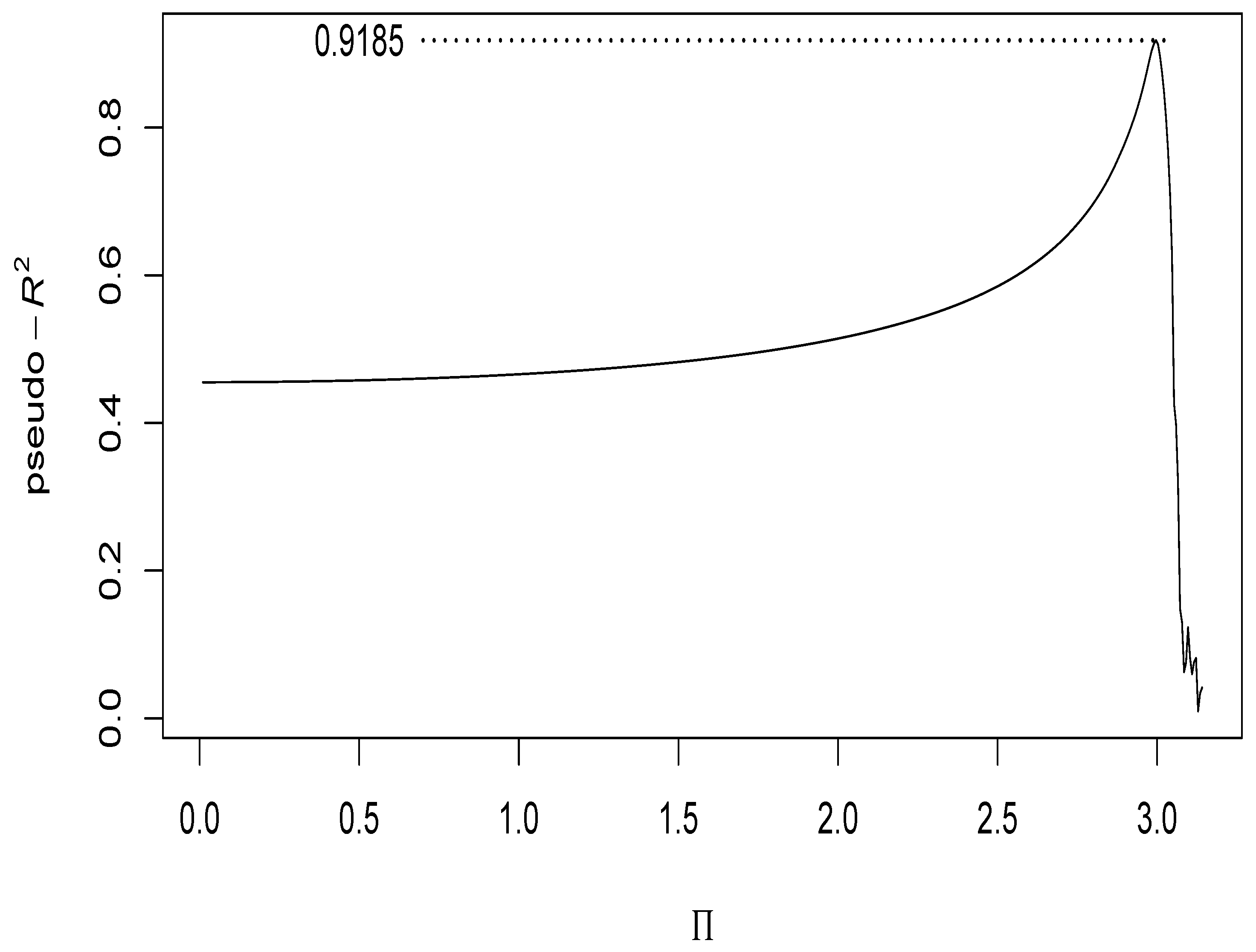
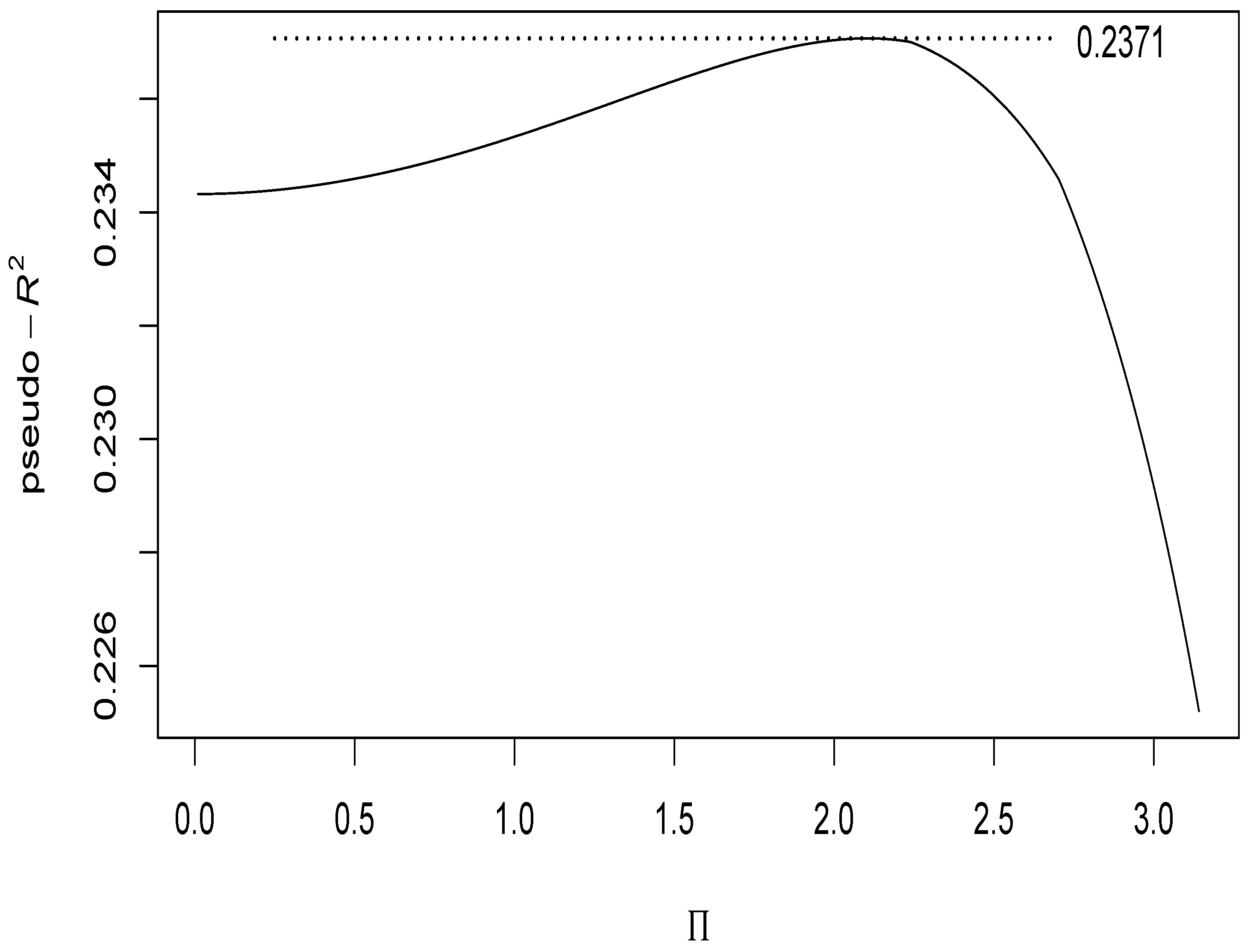
2.6. Choosing the Value for
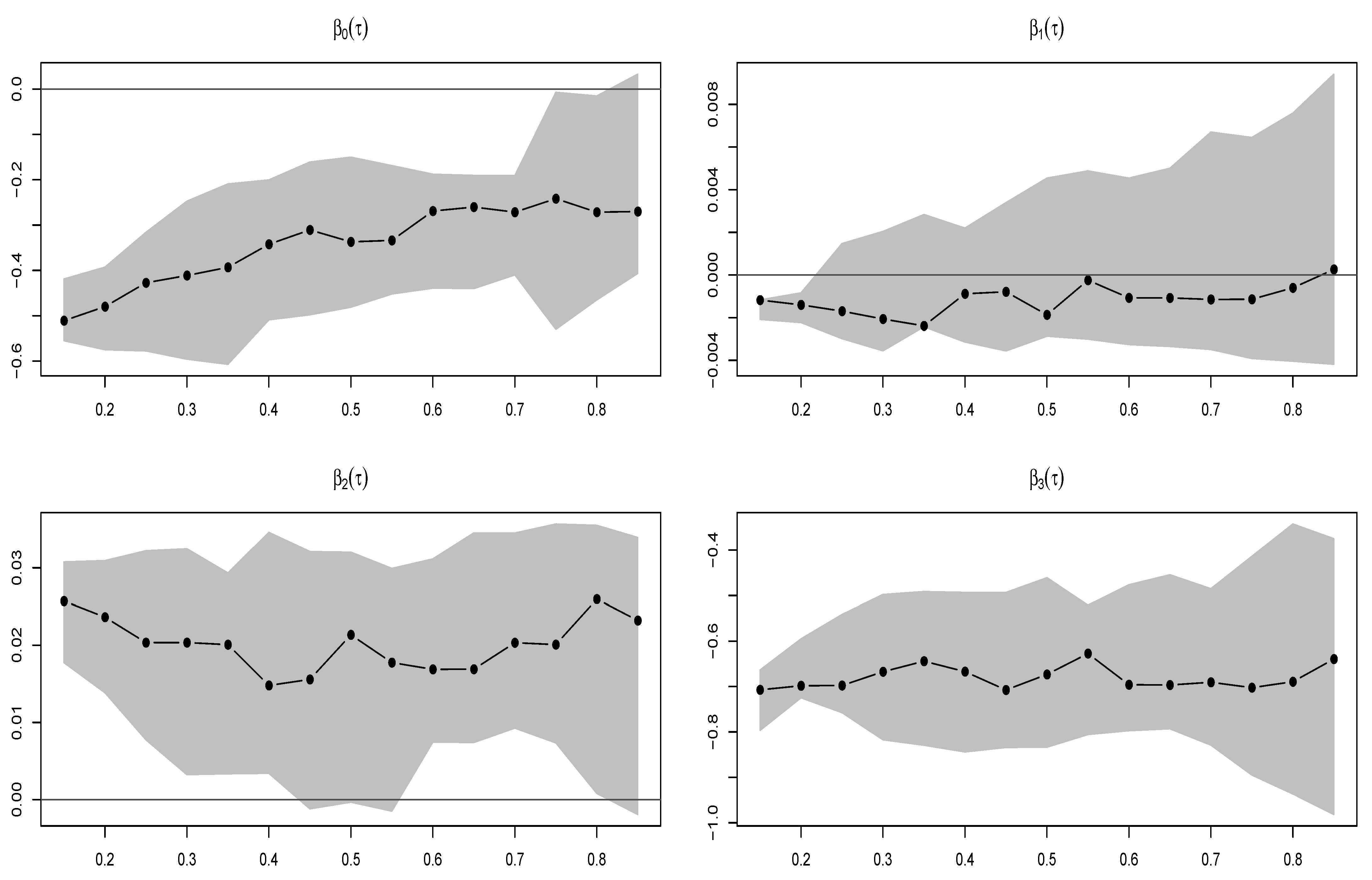
 Π

When estimating the formulation stated in (7), we initially assume that Π = 2.5 . Although Π can be chosen within the support ( 0 , π ) , a systematic approach would involve selecting the value that yields the best model fit. This selection can be evaluated using goodness-of-fit measures like the pseudo- R 2 or the Akaike information criterion (AIC).
Contrary to the traditional R 2 used in OLS regression, the pseudo- R 2 does not provide a proportion of variance explained by the model. Instead, it gives a measure of the deviation of the predicted values from the observed values, with larger values indicating a better fit. In contrast, the AIC is a measure that balances the fit of the model against its complexity. Generally, a model with a smaller AIC is considered to provide a better fit, given the number of parameters it utilizes.
For illustrative purposes, we consider a simulated dataset. The data were randomly generated from a normal distribution. Using β 1 ( 0.5 ) = 1 , β 2 ( 0.5 ) = 2 , β 3 ( 0.5 ) = 5 and the inverse of the function stated in (7), we generate the data y . Then, we produced n = 100 observations considering the seed 1234. Hence, the simulated data were estimated for τ = 0.5 , testing 500 different values for Π , uniformly distributed in the interval ( 0 , π ) . Figure 3 displays the values of Π used and the corresponding pseudo- R 2 values obtained. We observe a peak in the pseudo- R 2 at Π = 2.9972 , indicating that this is the optimal value for such a specific scenario.

3. Applications

This section illustrates the new fractile regression model using two datasets. The first dataset is presented in [33] and is related to household expenditure on food. These data are well known and were used in [34]. The second dataset is associated with the socioeconomic variables of 138 countries, and it was obtained from “The Quality of Government Basic Dataset”, Jan15 version (University of Gothenburg: The Quality of Government Institute, http://www.qog.pol.gu.se, accessed on 18 August 2023). With this dataset, we model the democratization index.

3.1. Application 1

In this application, we utilize the dataset presented in [33] which pertains to household expenditure on food. The response variable, denoted as Y, represents the proportion of income that a family spends on food.
To explain Y, we use two explanatory variables: the family income ( X 1 ) and the number of people in the family ( X 2 ) . The dataset consists of n = 38 observations, and it can be obtained from the betareg package of the R software [35,36], available on CRAN (https://www.r-project.org/, accessed on 18 August 2023).
Consider the fractile regression model formulated as
Q τ ( G ( Y i ) ) = β 0 ( τ ) + β 1 ( τ ) x i 1 + β 2 ( τ ) x i 2 , i { 1 , , 38 } .
We estimate three models, denoted by M1, M2, and M3, utilizing different link functions. Model M1 uses the link function stated in (5), model M2 employs the link function defined in (6), and model M3 applies the link function established in (7). Using the methodology described in Section 2.6, we employ Π = 2.1061 to estimate model M3. The performance of this estimation, reflected by the pseudo- R 2 values, is shown in Figure 4.
Observing Table 3, note that the estimated parameters are influenced by the choice of the link function. For model M1, one of the estimated parameters is statistically significant ( β 1 ). However, the estimates for β 1 and β 0 are statistically significant for model M2. All the estimated parameters for model M3 are statistically significant. Evaluating the goodness of fit using a pseudo- R 2 as a measure, model M1 exhibits the poorest fit, while models M2 and M3 have similar fits, with model M3 having a slight advantage. It is also noticed that the statistical significance of the parameters varies according to the chosen link function. The performance of these estimators, in terms of pseudo- R 2 values, is shown in Figure 4. Table 3 reports the estimates of models M1, M2, and M3 for the 50th fractile. The variation in the estimated parameters β 0 , β 1 , and β 2 with respect to τ for model M3 is depicted in Figure 5.

3.2. Application 2

In this application, we employ data from “The Quality of Government Basic Dataset” of the University of Gothenburg. These data are from n = 138 countries in the year 2010, where the response variable is a democratization index (Y), which can take values in [0, 1]. The covariates are real gross domestic product per capita in thousands of dollars ( X 1 ), average schooling (in years) of people aged 25 years or more ( X 2 ), and press freedom ( X 3 ). Note that X 3 is an index that takes values between zero and one, with a lower value indicating greater press freedom, while a higher value indicates limited press freedom.
Consider the fractile regression model formulated as
Q τ ( G ( Y i ) ) = β 0 ( τ ) + β 1 ( τ ) x i 1 + β 2 ( τ ) x i 2 + β 3 ( τ ) x i 3 , i { 1 , , 138 } .
We use the expressions stated in (5), (6), and (7) as link functions. Then, we estimate three models denoted by M4, M5, and M6. Once again, utilizing the methodology described in Section 2.6, we use Π = 1.4722 to estimate model M6, as shown in Figure 6. The estimation results of these models for the median (with their standard error in parentheses) and their corresponding pseudo- R 2 are reported in Table 4.
Note that the results of the estimates differ when different link functions are employed. Estimates for the parameters of model M4 indicate that only the values associated with X 2 and X 3 are statistically significant at a 10 % level. For models M5 and M6, all the estimates were found to be statistically significant at 10 % . Taking the pseudo- R 2 as a measure of the goodness of fit, it is observed that models M4 and M5 have a similar fit, while model M6 shows a better fit than models M4 and M5. Furthermore, it is once again evident that the statistical significance of the parameters varies depending on the chosen link function. Figure 7 illustrates the parameter estimates of model M6 across different fractiles. Observe that the estimated parameter associated with press freedom — β 3 ( τ ) — has a low variation between the lower and upper fractiles, demonstrating a consistent influence on democracies.

4. Concluding Remarks

In conclusion, this article have introduced an alternative approach to data modeling contained in the unit interval by extending the standard fractile regression model. We have addressed two criticisms of the methodology proposed in [24], when applied to data within the unit interval. We have also proposed alternative link functions to overcome these criticisms.
Our new approach has offered several advantages. First, it has allowed for direct interpretation of the model estimates in terms of the response variable, providing meaningful insights into the relationship between the covariates and the response. Second, our extensive simulation studies have shown that the approach demonstrated robustness when using different link functions, ensuring the stability and reliability of the estimated fractile regression coefficients even in simplified scenarios.
Another strength of the introduced approach is its independence from assumptions about the distribution of the response variable. This flexibility makes our approach applicable to a wide range of data scenarios, where the underlying distribution may be unknown or may deviate from traditional parametrical assumptions. Furthermore, the introduced approach addressed criticisms of the existing methods, offering a more robust and interpretable framework for data modeling within the unit interval.
The applications of the introduced approach to two real datasets have demonstrated its effectiveness and provided valuable insights into the modeling of household expenditure on food and democratization. The estimated models have yielded statistically significant coefficients and satisfactory goodness-of-fit measures, demonstrating the practical applicability of our new approach.
While our approach offers advantages, it may vary in efficacy depending on data characteristics. Its flexibility might not always be optimal for data with specific distributions, and there could be scenarios in which alternative methods might be preferable.
This investigation has focused on the development and illustration of the introduced approach. However, it is important to acknowledge that there are other existing approaches and methodologies for modeling data supported within limited intervals. Future research could involve comparative studies, where the introduced approach is compared with alternative methods specifically designed for modeling data within the unit interval. Such comparisons would provide a comprehensive evaluation of the performance and advantages of our approach, helping researchers select the most suitable method for their specific applications.
By recognizing the potential for comparisons and leveraging existing research in the field, we hope to contribute to the ongoing exploration and refinement of modeling techniques for bounded responses. The introduced approach, along with future comparative studies, can further enhance our understanding and ability to model data within the unit interval accurately.

Author Contributions

Conceptualization, J.S.C.d.O., R.O., V.L., J.F.-Z. and C.C.; data curation, J.S.C.d.O. and R.O.; formal analysis, J.S.C.d.O., R.O., V.L., J.F.-Z. and C.C.; investigation, J.S.C.d.O. and R.O.; methodology, J.S.C.d.O., R.O., V.L., J.F.-Z. and C.C.; writing-original draft, J.S.C.d.O., R.O. and J.F.-Z.; writing—review and editing, V.L. and C.C. All authors have read and agreed to the published version of the manuscript.

Funding

This research was partially supported by the National Council for Scientific and Technological Development (CNPq) through the grant 303192/2022-4 (R.O.); by FONDECYT grant number 1200525 (V.L.) from the National Agency for Research and Development (ANID) of the Chilean government under the Ministry of Science, Technology, Knowledge, and Innovation; and by Portuguese funds through the CMAT-Research Centre of Mathematics of University of Minho-within projects UIDB/00013/2020 and UIDP/00013/2020 (C.C.).

Institutional Review Board Statement

Not applicable.

Informed Consent Statement

Not applicable.

Data Availability Statement

Data and codes are available upon request from the authors.

Acknowledgments

The authors would also like to thank the editors and four reviewers for their constructive comments which led to the improvement of the presentation of the manuscript.

Conflicts of Interest

The authors declare no conflict of interest.

References

  1. Johnson, N.L.; Kotz, S.; Balakrishnan, N. Continuous Univariate Distributions; Wiley: New York, NY, USA, 1994; Volume 1. [Google Scholar]
  2. Johnson, N.L.; Kotz, S.; Balakrishnan, N. Continuous Univariate Distributions; Wiley: New York, NY, USA, 1995; Volume 2. [Google Scholar]
  3. Kotz, S.; Leiva, V.; Sanhueza, A. Two new mixture models related to the inverse Gaussian distribution. Methodol. Comput. Appl. Probab. 2010, 12, 199–212. [Google Scholar] [CrossRef]
  4. Mazucheli, J.; Menezes, A.F.; Dey, S. The unit-Birnbaum-Saunders distribution with applications. Chil. J. Stat. 2018, 9, 47–57. [Google Scholar]
  5. Shahin, A.I.; Almotairi, S. A deep learning BiLSTM encoding-decoding model for COVID-19 pandemic spread forecasting. Fractal Fract. 2021, 5, 175. [Google Scholar] [CrossRef]
  6. Ribeiro, T.F.; Cordeiro, G.M.; Peña-Ramírez, F.A.; Guerra, R.R. A new quantile regression for the COVID-19 mortality rates in the United States. Comput. Appl. Math. 2022, 40, 255. [Google Scholar] [CrossRef]
  7. Mazucheli, M.; Alves, B.; Menezes, A.F.B.; Leiva, V. An overview on parametric quantile regression models and their computational implementation with applications to biomedical problems including COVID-19 data. Comput. Methods Programs Biomed. 2022, 221, 106816. [Google Scholar] [CrossRef]
  8. Li, S.; Chen, J.; Li, B. Estimation and testing of random effects semiparametric regression model with separable space-time filters. Fractal Fract. 2022, 6, 735. [Google Scholar] [CrossRef]
  9. Jiang, J. Linear and Generalized Linear Mixed Models and Their Applications; Springer: New York, NY, USA, 2006. [Google Scholar]
  10. Leiva, V.; Rojas, E.; Galea, M.; Sanhueza, A. Diagnostics in Birnbaum-Saunders accelerated life models with an application to fatigue data. Appl. Stoch. Model. Bus. Ind. 2014, 30, 115–131. [Google Scholar] [CrossRef]
  11. Ramalho, E.A.; Ramalho, J.J.; Murteira, J.M. Alternative estimating and testing empirical strategies for fractional regression models. J. Econ. Surv. 2011, 25, 19–68. [Google Scholar] [CrossRef]
  12. Papke, L.E.; Wooldridge, J. Econometric methods for fractional response variables with an application to 401(k) plan participation rates. J. Appl. Econom. 1996, 11, 619–632. [Google Scholar] [CrossRef]
  13. Ferrari, S.; Cribari-Neto, F. Beta regression for modelling rates and proportions. J. Appl. Stat. 2004, 31, 799–815. [Google Scholar] [CrossRef]
  14. Smithson, M.; Verkuilen, J. A better lemon squeezer? Maximum-likelihood regression with beta-distributed dependent variables. Psychol. Methods 2006, 11, 54–71. [Google Scholar] [CrossRef] [PubMed]
  15. Mazucheli, J.; Menezes, A.F.B.; Chakraborty, S. On the one parameter unit-Lindley distribution and its associated regression model for proportion data. J. Appl. Stat. 2019, 46, 700–714. [Google Scholar] [CrossRef]
  16. Altun, E.; El-Morshedy, M.; Eliwa, M. A new regression model for bounded response variable: An alternative to the beta and unit-Lindley regression models. PLoS ONE 2021, 16, e0245627. [Google Scholar] [CrossRef] [PubMed]
  17. Ospina, R.; Ferrari, S.L. A general class of zero-or-one inflated beta regression models. Comput. Stat. Data Anal. 2012, 56, 1609–1623. [Google Scholar] [CrossRef]
  18. Korkmaz, M.; Chesneau, C. On the unit Burr-XII distribution with the quantile regression modeling and applications. Comput. Appl. Math. 2021, 40, 29. [Google Scholar] [CrossRef]
  19. Korkmaz, M.; Korkmaz, Z.S. The unit log-log distribution: A new distribution with alternative quantile regression modeling and educational measurements applications. J. Appl. Stat. 2023, 50, 889–908. [Google Scholar] [CrossRef]
  20. Leiva, V.; Mazucheli, J.; Alves, B. A novel regression model for fractiles: Formulation, computational aspects, and applications to medical data. Fractal Fract. 2023, 7, 169. [Google Scholar] [CrossRef]
  21. Korkmaz, M.; Leiva, V.; Martin, C. The continuous Bernoulli distribution: Mathematical characterization, fractile regression, computational simulations, and applications. Fractal Fract. 2023, 7, 386. [Google Scholar] [CrossRef]
  22. Saulo, H.; Vila, R.; Bittencourt, V.; Leao, J.; Leiva, V.; Christakos, G. On a new extreme value distribution: Characterization, parametric quantile regression, and application to extreme air pollution events. Stoch. Environ. Res. Risk Assess. 2023, 37, 1119–1136. [Google Scholar] [CrossRef]
  23. Saulo, H.; Vila, R.; Borges, G.; Bourguignon, M.; Leiva, V.; Marchant, C. Modeling income data via new quantile regressions: Formulation, computation, and application. Mathematics 2023, 11, 448. [Google Scholar] [CrossRef]
  24. Bottai, M.; Cai, B.; McKeown, R.E. Logistic quantile regression for bounded outcomes. Stat. Med. 2010, 29, 309–317. [Google Scholar] [CrossRef] [PubMed]
  25. Lindsey, J.K. Applying Generalized Linear Models; Springer: New York, NY, USA, 2000. [Google Scholar]
  26. Koenker, R.; Bassett, G. Regression quantiles. Econometrica 1978, 46, 33–50. [Google Scholar] [CrossRef]
  27. Koenker, R. Quantile Regression; Cambridge University Press: Cambridge, UK, 2005. [Google Scholar]
  28. Bonat, W.H.; Lopes, J.E.; Shimakura, S.E.; Ribeiro, P.J., Jr. Likelihood analysis for a class of simplex mixed models. Chil. J. Stat. 2018, 9, 3–17. [Google Scholar]
  29. dos Santos, A.R.P.; de Faria, R.Q.; Amorim, D.J.; Giandoni, V.C.R.; da Silva, E.A.A.; Sartori, M.M.P. Cauchy, Cauchy-Santos-Sartori-Faria, logit, and probit functions for estimating seed longevity in soybean. Agron. J. 2019, 111, 2929–2939. [Google Scholar] [CrossRef]
  30. Shoemaker, A.C. Effects of misspecification of the link function in models for binomial data. J. Stat. Plan. Inference 1984, 33, 213–231. [Google Scholar]
  31. Koenker, R. Quantreg: Quantile Regression. R Package Version 5.86. 2021. Available online: https://CRAN.R-project.org/package=quantreg (accessed on 13 July 2023).
  32. Cox, D.R.; Hinkley, D.V. Theoretical Statistics; CRC Press: Boca-Raton, FL, USA, 1979. [Google Scholar]
  33. Griffiths, W.; Hill, C.; Judge, R.; Griffiths, G.G.W.; Hill, R.C.; Judge, G.G. Learning and Practicing Econometrics; Wiley: New York, NY, USA, 1993. [Google Scholar]
  34. Cribari-Neto, F.; Zeileis, A. Beta regression in R. J. Stat. Softw. 2010, 34, 1–24. [Google Scholar] [CrossRef]
  35. R Core Team. R: A Language and Environment for Statistical Computing; R Foundation for Statistical Computing: Vienna, Austria, 2022; Available online: www.r-project.org (accessed on 18 August 2023).
  36. Korosteleva, O. Advanced Regression Models with SAS and R; CRC Press: Boca Raton, FL, USA, 2019. [Google Scholar]
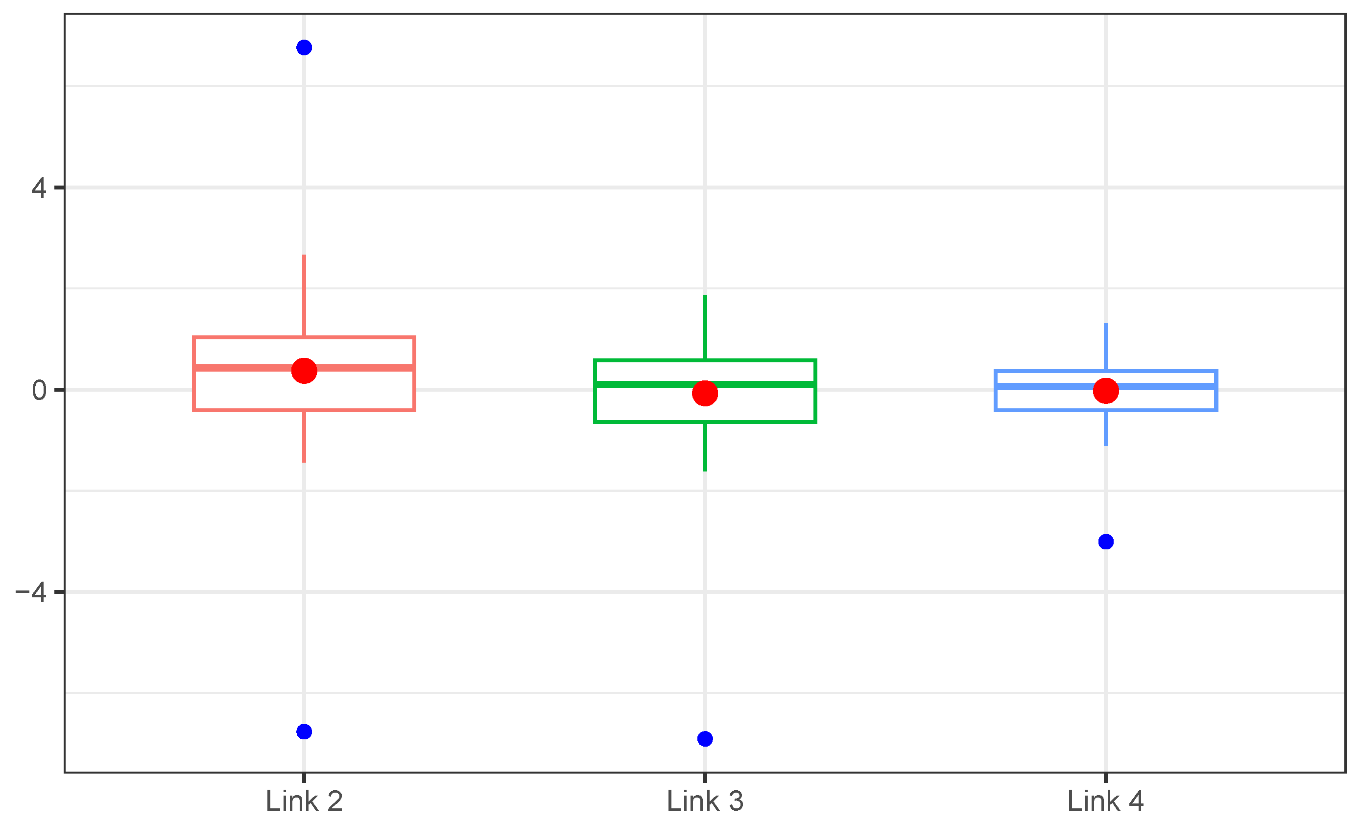
Figure 1. Boxplots of the transformed variable Y using the link functions stated in (5) –Link 2 colored in light red–, (6) –Link 3 colored in green–, and (7) –Link 4 colored in light blue–, where the red points represent the data mean, while the blue points indicate outliers.
Fractalfract 07 00667 g001
Figure 2. Flowchart illustrating the detailed estimation process of the fractile regression parameters.
Fractalfract 07 00667 g002
Figure 3. Plot of the values of Π versus their corresponding pseudo- R 2 values.
Fractalfract 07 00667 g003
Figure 4. Plot of the values of Π versus their corresponding pseudo- R 2 values in model M3.
Fractalfract 07 00667 g004
Figure 5. Plots of the estimated parameters β 0 , β 1 , and β 2 (in black lines and points) as functions of the indicated fractile τ for model M3, where the gray zone corresponds to a 90% confidence band for the listed parameter.
Fractalfract 07 00667 g005
Figure 6. Plot of the values of Π versus their corresponding pseudo- R 2 values in model M6.
Fractalfract 07 00667 g006
Figure 7. Plots of the estimated parameters β 0 , β 1 , β 2 , and β 3 (in black lines and points) as functions of the indicated fractile τ for model M6, where the gray zone corresponds to a 90% confidence band for the listed parameter.
Fractalfract 07 00667 g007
Table 1. Descriptive statistics of the data and their transformation using the indicated link function.
LinkMinimumQuartile 1MedianMeanQuartile 3Maximum
Identity 0.0000 0.3451 0.5252 0.5012 0.6402 0.8670
Logit 6.7660 0.4128 0.4288 0.3713 1.0350 6.7660
Logit 2 6.9090 0.6395 0.1008 0.0740 0.5749 1.8680
Cauchy 3.0100 0.4080 0.0632 0.0242 0.3655 1.3060
Table 2. Empirical mean (M), bias (B), and mean squared error (MSE) of the estimators of θ τ based on Monte Carlo simulations and the model Q τ ( G ( Y ) x ) = β 1 ( τ ) x 1 + β 2 ( τ ) x 2 + β 3 ( τ ) x 3 , for the indicated values of n, τ , β 1 , β 2 , and β 3 .
θ 0.5 θ 0.25
β 1 ( 0 . 5 ) β 2 ( 0 . 5 ) β 3 ( 0 . 5 ) β 1 ( 0 . 25 ) β 2 ( 0 . 25 ) β 3 ( 0 . 25 )
1.5000 2 . 5000 1 . 9000 0 . 5000 0 . 5000 0 . 9000
M( θ ^ τ ) 1.4988 2.5006 1.9020 0.5073 0.5012 0.8993
n = 40 B( θ ^ τ ) 0.0012 0.0006 0.0020 0.0073 0.0012 0.0007
MSE( θ ^ τ ) 0.0518 0.0089 0.0135 0.0687 0.0158 0.0144
M( θ ^ τ ) 1.4993 2.5000 1.8991 0.5042 0.4997 0.9001
n = 60 B( θ ^ τ ) 0.0007 0.0000 0.0009 0.0042 0.0003 0.0001
MSE( θ ^ τ ) 0.0299 0.0067 0.0063 0.0406 0.0086 0.0077
M( θ ^ τ ) 1.5003 2.5008 1.8991 0.5029 0.5004 0.8989
n = 100 B( θ ^ τ ) 0.0003 0.0008 0.0009 0.0029 0.0004 0.0011
MSE( θ ^ τ ) 0.0226 0.0055 0.0047 0.0223 0.0048 0.0055
M( θ ^ τ ) 1.5010 2.5001 1.8998 0.4992 0.5002 0.8999
n = 200 B( θ ^ τ ) 0.0010 0.0001 0.0002 0.0008 0.0002 0.0001
MSE( θ ^ τ ) 0.0102 0.0020 0.0019 0.0108 0.0027 0.0023
M( θ ^ τ ) 1.5006 2.5000 1.9005 0.4957 0.4997 0.9005
n = 500 B( θ ^ τ ) 0.0006 0.0000 0.0005 0.0043 0.0003 0.0005
MSE( θ ^ τ ) 0.0040 0.0008 0.0008 0.0049 0.0010 0.0009
Table 3. Estimates for the parameters of models M1, M2, and M3 at 50th fractile, where * indicates significance at the 10% level and standard errors are shown in parentheses below the estimates.
ParameterM1M2M3
EstimateE m EstimateE m EstimateE m
β 0 0.13490.0150−0.6143 *−0.1293−0.3250 *−0.1285
(0.5075) (0.2632) (0.1408)
β 1 −0.0181 *−0.0020−0.0094 *−0.0020−0.0050 *−0.0020
(0.0077) (0.0039) (0.0021)
β 2 0.17620.01970.08890.01870.0473 *0.0187
(0.1108) (0.0557) (0.0296)
Pseudo- R 2 0.17010.23530.2371
Table 4. Estimates for the parameters of models M4, M5, and M6 at 50th fractile, where * indicates significance at the 10% level and standard errors are shown in parentheses below the estimates.
ParameterM4M5M6
EstimateE m EstimateE m EstimateE m
β 0 0.49480.0538−0.6968 *−0.0924−0.3370 *−0.1811
(0.3048) (0.2074) (0.0715)
β 1 −0.0079−0.0009−0.0116 *−0.0015−0.0019−0.0010
(0.0119) (0.0061) (0.0015)
β 2 0.1101 *0.01200.0731 *0.00970.0213 *0.0115
(0.0359) (0.0237) (0.0067)
β 3 −3.7126 *−0.4038−2.9549 *−0.3918−0.6733 *−0.3617
(0.4492) (0.3347) (0.0752)
Pseudo- R 2 0.30910.30360.4396
Disclaimer/Publisher’s Note: The statements, opinions and data contained in all publications are solely those of the individual author(s) and contributor(s) and not of MDPI and/or the editor(s). MDPI and/or the editor(s) disclaim responsibility for any injury to people or property resulting from any ideas, methods, instructions or products referred to in the content.

