Fractional Pricing Models: Transformations to a Heat Equation and Lie Symmetries

Abstract

The study of fractional partial differential equations is often plagued with complicated models and solution processes. In this paper, we tackle how to simplify a specific parabolic model to facilitate its analysis and solution process. That is, we investigate a general time-fractional pricing equation, and propose new transformations to reduce the underlying model to a different but equivalent problem that is less challenging. Our procedure leads to a conversion of the model to a fractional 1 + 1 heat transfer equation, and more importantly, all the transformations are invertible. A significant result which emerges is that we prove such transformations yield solutions under the Riemann–Liouville and Caputo derivatives. Furthermore, Lie point symmetries are necessary to construct solutions to the model that incorporate the behaviour of the underlying financial assets. In addition, various graphical explorations exemplify our results.

1. Introduction

In recent times, fractional-based models are at the forefront in financial modelling. Such models display two very important properties: self-similarity and long-range dependence [1,2,3]. In [4], it was further posed that stock price volatility is well described by fractional Brownian motion since it has random-like features to portray uneven fluctuations in stock price. This is one of the many reasons why fractional derivatives are preferred in many spheres. Moreover, based on the collective arguments in the literature, such as [5,6,7,8], the time-fractional Black–Scholes equation is consistent with the integer-order Black–Scholes model in the limit as the order of the fractional derivative tends to one. In [9], the fractional Black–Scholes equation was solved by using the Green’s function.

Taking into account the above discussion, we consider the general fractional bond pricing equation

$$\begin{array}{c}\hfill \frac{{\partial }^{\alpha }V}{\partial t^{\alpha }}+\frac{1}{2}{\rho }^2{S}^{2\gamma }\frac{{\partial }^{2}V}{\partial S^2}+\left(\kappa -\lambda \rho S^{\gamma }+\beta S\right)\frac{\partial V}{\partial S}-SV=0,V(S,t),\end{array}$$

(1)

where $\kappa ,\beta ,\rho ,\lambda$ (the market price of risk) and $\gamma$ are constants, t is time, S is the stock price or instantaneous short-term interest rate at current time t and $V(S,t)$ is the current value of the bond. As expected, $\alpha (0<\alpha <1)$ is the order of the fractional derivative, and an integer order model is obtained for $\alpha =1$.

Equation (1) is a parabolic partial differential equation (PDE) with various versions, for example, the Vasicek $\gamma =0$, Dothan $\kappa =\beta =0,\gamma =1$ and Cox–Ingersoll model $\gamma =1/2$, $\lambda =0$ [10,11,12,13]. In [14], the above model was considered subject to classical derivatives and a boundary condition.

Transformations are a fascinating subject, and have been the central driving force of mathematics for more than a century. In the 19th century in particular, the concept of transformations and permutations led to groundbreaking mathematical advancements, i.e., the discovery of new geometries and algebraic instruments. Since then, the study of transformations has grown in leaps and bounds. As an instrument in the study of all possible types of differential equations, transformations are the heart and soul of analytical solution techniques. Furthermore, transformative methods may sometimes be used in conjunction with numerical approaches. Explicitly, transformations simplify the equation, either by creating an easier form of the equation, or through combining variables, and thereby decreasing the number of variables. The only challenge, of course, is the calculation of such transformations.

In this paper, we construct several transformations that are crucial in simplifying the above model. We also apply another type of transformation later on in the study, this time calculated from symmetry methods [15]. In a profound and unique way, a symmetry of a differential equation is a transformation (or mapping) of its solution manifold into itself.

The aim of this paper is twofold: firstly, to construct equivalence formulae that transforms the given fractional equation into a fractional heat transfer equation. This process is, to the best of our knowledge, the first of its kind for this model. Secondly, through rigorous mathematical proofs, we provide symmetry invariant solutions to the original equation. To support these theoretical observations, graphical examples are presented under the proposed fractional framework. Results indicate that such a study is highly effective in financial modelling.

The plan of the paper is as follows. In Section 2, we note the fractional derivatives to be applied in the theory below. Section 3 is the main section, where we introduce the parameters and transformations required to manipulate the fractional model (1) into the fractional heat equation. We further define some elementary properties of the heat equation followed by novel symmetry-generated solutions of the pricing model (1). Finally, in Section 4, we end with a meaningful discussion of the obtained solutions.

2. Preliminaries

We define the two fractional derivatives used in this paper, more detailed properties of these derivatives are well-known and can be found in the literature cited here. We note that many other fractional derivates exist, but we limit ourselves to two of the most popular ones. A wealth of knowledge on fractional calculus can be found in the texts [16,17] to establish a comprehensive grasp of the subject material. Let $\alpha$ be any positive real number and n be a natural number such that $n-1\le \alpha <n$.

The Riemann–Liouville derivative of order $\alpha$ is defined as [18]:

$$D_t^{\alpha }u(t,x)=\frac{1}{\Gamma (n-\alpha )}\frac{{\partial }^n}{\partial t^n}{\int }_0^t{(t-\tilde{\tau })}^{n-\alpha -1}u(\tilde{\tau },x)d\tilde{\tau }.$$

(2)

Similarly, the Caputo derivative of order $\alpha$ is defined as [18]:

$$D_t^{\alpha }u(t,x)=\frac{1}{\Gamma (n-\alpha )}{\int }_0^t{(t-\tilde{\tau })}^{n-\alpha -1}\frac{{\partial }^n}{\partial t^n}u(\tilde{\tau },x)d\tilde{\tau }.$$

(3)

The methods used involve symmetries of differential equations, which have been extended to FDEs by the works [19,20,21,22], both in the Riemann–Liouville and Caputo sense, with interesting discussions in the publications [23,24,25].

First, we recall the basic theory for finding symmetries under a Riemann–Liouville time-fractional derivative. Consider the equation

$$\frac{{\partial }^{\alpha }u}{\partial t^{\alpha }}=M\left(x,t,u,u_x,u_{xx}\right),$$

(4)

where $0<\alpha <1$ is the parameter describing the order of the fractional time derivative.

Suppose that (4) is invariant under the one-parameter Lie group of point transformations:

$$\begin{array}{cc}\hfill \overline{t}=& t+ϵ\tau (x,t,u)+O\left({ϵ}^2\right),\\ \hfill \overline{x}=& x+ϵ\xi (x,t,u)+O\left({ϵ}^2\right),\\ \hfill \overline{u}=& u+ϵ\eta (x,t,u)+O\left({ϵ}^2\right),\\ \hfill \frac{{\partial }^{\alpha }\overline{u}}{\partial {\overline{t}}^{\alpha }}=& \frac{{\partial }^{\alpha }u}{\partial t^{\alpha }}+ϵ{\eta }_{\alpha }^0(x,t,u)+O\left({ϵ}^2\right),\\ \hfill \frac{\partial \overline{u}}{\partial \overline{x}}=& \frac{\partial u}{\partial x}+ϵ{\eta }^x(x,t,u)+O\left({ϵ}^2\right),\\ \hfill \frac{{\partial }^2\overline{u}}{\partial {\overline{x}}^2}=& \frac{{\partial }^{2}u}{\partial x^2}+ϵ{\eta }^{xx}(x,t,u)+O\left({ϵ}^2\right),\end{array}$$

(5)

where $ϵ$ is an infinitesimal parameter, and the standard prolongation formulae are:

$$\begin{array}{ccc}\hfill {\eta }^x& =& {\eta }_x+{\eta }_u{u}_x-\left({\xi }_x+{\xi }_u{u}_x\right)u_x-\left({\tau }_x+{\tau }_u{u}_x\right)u_t,\hfill \\ \hfill {\eta }^{xx}& =& {\eta }_{xx}+2{\eta }_{xu}{u}_x-2{\xi }_{xu}{u_x}^2-{\xi }_{xx}{u}_x-2{\tau }_{ux}{u}_t{u}_x-{\tau }_{xx}{u}_t-{\xi }_{uu}{u_x}^3\hfill \\ & & -{\tau }_{uu}{u_x}^2{u}_t+{\eta }_{uu}{u_x}^2-3{\xi }_u{u}_x{u}_{xx}-{\tau }_u{u}_t{u}_{xx}+{\eta }_u{u}_{xx}-2{\xi }_x{u}_{xx}\hfill \\ & & -2{\tau }_u{u}_x{u}_{tx}-2{\tau }_x{u}_{tx}.\hfill \end{array}$$

(6)

By the generalised Leibniz rule and a generalisation of the chain rule, the prolongation formula under the Riemann–Liouville formulation is also [20]

$$\begin{array}{ccc}\hfill {\eta }_{\alpha }^0& =& \frac{{\partial }^{\alpha }\eta }{\partial t^{\alpha }}+\left(\eta -\alpha D_t\left(\tau \right)\right)\frac{{\partial }^{\alpha }u}{\partial t^{\alpha }}-u\frac{{\partial }^{\alpha }{\eta }_u}{\partial t^{\alpha }}+\mu +\sum _{n=1}^{\infty }\left(\genfrac{}{}{0pt}{}{\alpha }{n}\right)D_t^n\left(\xi \right)D_t^{\alpha -n}\left(u_x\right)\hfill \\ & & +\sum _{n=1}^{\infty }\left[\left(\genfrac{}{}{0pt}{}{\alpha }{n}\right)\frac{{\partial }^n}{\partial t^n}{\eta }_u-\left(\genfrac{}{}{0pt}{}{\alpha }{n+1}\right)D_t^{n+1}\left(\tau \right)\right]D_t^{\alpha -n},\hfill \end{array}$$

(7)

and

$$\begin{array}{cc}\hfill \mu & ={\sum }_{n=2}^{\infty }{\sum }_{m=2}^n{\sum }_{k=2}^m{\sum }_{r=0}^{k-1}\left(\genfrac{}{}{0pt}{}{\alpha }{n}\right)\left(\genfrac{}{}{0pt}{}{n}{m}\right)\left(\genfrac{}{}{0pt}{}{k}{r}\right)\frac{1}{k!}\frac{t^{n-\alpha }}{\Gamma \left(n+1-\alpha \right)}\\ & \phantom{aa}\times {(-u)}^r\frac{{\partial }^m}{\partial t^m}\left(u^{k-r}\right)\frac{{\partial }^{n-m+k}\eta }{\partial t^{n-m}\partial u^k}.\end{array}$$

(8)

By convention, $\eta (x,t,u)$ is assumed to be linear in the variable u, so that $\mu$ vanishes. Let the symmetry generator

$$\begin{array}{c}\hfill X=\tau (x,t,u)\frac{\partial }{\partial t}+\xi (x,t,u)\frac{\partial }{\partial x}+\eta (x,t,u)\frac{\partial }{\partial u}\end{array}$$

(9)

span the associated Lie algebra, and

$$\tau (x,t,u)=\frac{d{t}^{*}}{dϵ}{|}_{ϵ=0},\xi (x,t,u)=\frac{d{x}^{*}}{dϵ}{|}_{ϵ=0},\eta (x,t,u)=\frac{d{u}^{*}}{dϵ}{|}_{ϵ=0}.$$

Let $H=\frac{{\partial }^{\alpha }u}{\partial t^{\alpha }}-M\left(x,t,u,u_x,u_{xx}\right)$; then, the infinitesimal criterion for invariance to determine symmetries is expressed as $XH=0,\mathrm{when}H=0,$ and where X is extended to all derivatives appearing in the equation through the appropriate prolongation. Moreover, the transformation (5) leaves invariant the lower limit of the fractional derivative $\frac{{\partial }^{\alpha }u}{\partial t^{\alpha }}$, i.e., we have the additional constraint:

$$\tau (x,t,u){|}_{t=0}=0.$$

(10)

This procedure is algorithmic and yields the symmetries of a time-fractional equation.

The method outlined above is similar if the fractional derivative is Caputo, but with different general prolongation formulae—see [22] for full details. However, the most important notion is that both of these derivatives produce the same Lie point symmetries, so that symmetry calculations using just one of the derivatives is sufficient.

3. Main Results—New Transformations

This section has three parts to it: firstly, we establish the required transformations to change the above model into the 1 + 1 time-fractional heat transfer equation; secondly, we list the Lie group details that are relevant for our version of the fractional and classical heat equation in order to take our study further. Finally, we prove several theorems on the resulting solutions of Equation (1).

3.1. Transformation of Equation (1)

In this section, we establish successive transformations that convert Equation (1) to a version of the heat equation. The change of variables is necessary to apply some interesting symmetry results to the model (1). It turns out that (1) is transformable under certain forms of its arbitrary parameters. Hence, we prove the following result.

Theorem 1.

The fractional pricing model Equation (1) is reducible to the fractional heat equation

$$\frac{{\partial }^{\alpha }\omega }{\partial {\widehat{t}}^{\alpha }}-\frac{1}{\Gamma (\alpha +1)}\frac{{\partial }^2\omega }{\partial y^2}=0,\omega \equiv \omega (y,\widehat{t}),$$

(11)

under the specific parameter settings, viz. $\gamma =2,\kappa =\beta =0,\lambda =-\frac{1}{\rho },$ and $\rho$ is arbitrary. The transformations are

$$\widehat{t}=-t^{\alpha },$$

(12)

$$y=-\frac{\sqrt{2}}{S\rho }.$$

(13)

Proof. 

A transformation of the independent variables of the form y and $\widehat{t}$ reduces Equation (1) to

$$a\left(y\right)\frac{\partial V}{\partial y}+c\left(y\right)V+\Gamma (\alpha +1)\frac{{\partial }^{\alpha }V}{\partial {\widehat{t}}^{\alpha }}-\frac{{\partial }^{2}V}{\partial y^2}=0,$$

(14)

where $V(y,\widehat{t})$,

$${\displaystyle a\left(y\right)=y\left(-\frac{2}{y^2}-\frac{\sqrt{2}}{y\rho }\right),}$$

and

$${\displaystyle c\left(y\right)=-\frac{\sqrt{2}}{y\rho }.}$$

Thereafter, we let

$$V(y,\widehat{t})=\omega (y,\widehat{t})·e^{-\varphi (y,\widehat{t})},$$

where

$$\varphi (y,\widehat{t})=\frac{y}{\sqrt{2}\rho }+log\left(y\right)+\frac{{\widehat{t}}^{\alpha }}{2{\rho }^2\alpha \Gamma \left(\alpha \right)\Gamma (\alpha +1)},$$

(15)

and the result follows that Equation (1) is converted to the fractional heat Equation (11). □

3.2. The Heat Equation

The classical heat equation has appeared in many studies [26,27], and a fourth-order nonlocal heat model was recently explored in [28]. Indeed, we showcase here that the heat equation is of the most useful of PDEs. Equation (11) shares some group properties with the classical integer-order heat equation.

The Lie point symmetries of (11) are well known for $\alpha =1$; they are:

$$\begin{array}{cc}& Z_1=\frac{\partial }{\partial y},Z_2=\frac{\partial }{\partial \widehat{t}},Z_3=\omega \frac{\partial }{\partial \omega },\\ & \\ & Z_4=y\frac{\partial }{\partial y}+2\widehat{t}\frac{\partial }{\partial \widehat{t}},\\ & \\ & Z_5=2\widehat{t}\frac{\partial }{\partial y}-y\omega \frac{\partial }{\partial \omega },\\ & \\ & Z_6=4\widehat{t}y\frac{\partial }{\partial y}+4{\widehat{t}}^2\frac{\partial }{\partial \widehat{t}}-(y^2+2\widehat{t})\omega \frac{\partial }{\partial \omega },\\ & \\ & Z_{\theta }=\theta (y,\widehat{t})\frac{\partial }{\partial \omega },\end{array}$$

(16)

where $\theta$ is an arbitrary solution of the heat equation, i.e., ${\theta }_{\widehat{t}}={\theta }_{yy}.$ The first six symmetries form a six-dimensional Lie algebra with the last symmetry spanning an infinite-dimensional sub-algebra. The commutator relations are presented in

Table 1. Lie commutator table for the symmetries of (11) when $\alpha =1$.

$(,)$	${\mathit{Z}}_1$	${\mathit{Z}}_2$	${\mathit{Z}}_3$	${\mathit{Z}}_4$	${\mathit{Z}}_5$	${\mathit{Z}}_6$
$Z_1$	0	0	0	$Z_1$	${-Z}_3$	${2Z}_5$
$Z_2$	0	0	0	${2Z}_2$	${2Z}_1$	$4Z_4-2Z_3$
$Z_3$	0	0	0	0	0	0
$Z_4$	${-Z}_1$	${-2Z}_2$	0	0	$Z_5$	${2Z}_6$
$Z_5$	$Z_3$	${-2Z}_1$	0	${-Z}_5$	0	0
$Z_6$	${-Z}_5$	$2Z_3-4Z_4$	0	$-2Z_6$	0	0

.

For $0<\alpha <1$, following the procedure from Section 2, the Lie point symmetries of (11) are:

$$Z_1,Z_3,Z_7=2\widehat{t}\frac{\partial }{\partial \widehat{t}}+\alpha y\frac{\partial }{\partial y},Z_{\theta }.$$

(17)

The first 3 symmetries form a 3-dimensional Lie algebra with the last symmetry spanning an infinite-dimensional sub-algebra. The commutator relations are in

Table 2. Lie commutator table for the symmetries of (11) when $0<\alpha <1$.

$[,]$	${\mathit{Z}}_1$	${\mathit{Z}}_7$	${\mathit{Z}}_3$
$Z_1$	0	${\alpha Z}_1$	0
$Z_7$	${-\alpha Z}_1$	0	0
$Z_3$	0	0	0

.

3.3. Invariant and Mittag-Leffler Solutions

Next, we consider a linear combination of symmetries $Z=Z_1+b{Z}_3$ (b is an arbitrary constant), and the method of invariants yields the transformation

$$\omega (y,\widehat{t})=\psi \left(\widehat{t}\right)e^{by},$$

(18)

so that Equation (11) becomes the fractional ordinary differential equation (FODE):

$$D_{\widehat{t}}^{\alpha }\psi \left(\widehat{t}\right)-\frac{b^2}{\Gamma (\alpha +1)}\psi \left(\widehat{t}\right)=0.$$

(19)

Theorem 2.

A solution $V(S,t)$ for the general pricing Equation (1) for $\alpha =1$, and under the parameters $\gamma =2,\kappa =\beta =0,\lambda =-\frac{1}{\rho },C$, and ρ are arbitrary, is the invariant solution:

$$V(S,t)=-\frac{C\rho S}{\sqrt{2}}exp\left(-b^{2}t-\frac{\sqrt{2}b}{\rho S}+\frac{1}{{\rho }^{2}S}+\frac{t}{2{\rho }^2}\right).$$

(20)

Proof. 

Since the symmetry generators $Z_1$ and $Z_3$ occur for integer-order derivatives, the combination $Z=Z_1+b{Z}_3$ can be used to reduce the classical heat equation:

$${\omega }_{\widehat{t}}-{\omega }_{yy}=0.$$

In this case, the reduction procedure leads to Equation (19) with $\alpha =1$, and hence, the solution becomes:

$$\psi \left(\widehat{t}\right)=Cexp\left(b^2\widehat{t}\right),$$

and Equation (18) presents that the classical heat equation has a solution of the form

$$\omega (y,\widehat{t})=Cexp\left(b^2\widehat{t}+by\right).$$

(21)

By Theorem 1, we reverse all transformations, and the result follows. □

An analogous result may be found for fractional-order derivatives. When $0<\alpha <1$, the solution of Equation (19) depends on the type of fractional derivative. Thus, we establish the following theorems and we note that as $\alpha \to 1$ in the theory below, we recover Theorem 2.

Theorem 3.

The general fractional pricing Equation (1), under a Riemann–Liouville fractional derivative with $0<\alpha <1$, and parameters $\gamma =2,\kappa =\beta =0,\lambda =-\frac{1}{\rho }$, and ρ arbitrary, admits the invariant solution:

$$V(S,t)=-\frac{C\rho S}{\sqrt{2}}{\left(-t^{\alpha }\right)}^{\alpha -1}{E}_{\alpha ,\alpha }\left(\frac{b^2{\left(-t^{\alpha }\right)}^{\alpha }}{\Gamma (\alpha +1)}\right)exp\left(-\frac{\sqrt{2}b}{\rho S}+\frac{1}{{\rho }^{2}S}-\frac{{\left(-t^{\alpha }\right)}^{\alpha }}{2\alpha {\rho }^2\Gamma \left(\alpha \right)\Gamma (\alpha +1)}\right).$$

(22)

Proof. 

Under the Riemann–Liouville derivative, the solution of the FODE (19) is given by Laplace transforms, as

$$\psi \left(\widehat{t}\right)=C{\widehat{t}}^{\alpha -1}{E}_{\alpha ,\alpha }\left(\frac{b^2}{\Gamma (\alpha +1)}{\widehat{t}}^{\alpha }\right),$$

(23)

where $C=D^{-(1-\alpha )}\psi \left(0\right)$ [29], and $E_{\alpha ,\alpha }$ is the generalised Mittag-Leffler function defined as

$$E_{\alpha ,\alpha }\left(z\right)=\sum _{k=0}^{\infty }\frac{z^k}{\Gamma (\alpha k+\alpha )},$$

(24)

with $\alpha >0.$ From (18), the solution of the fractional heat Equation (11) becomes

$$\omega (y,\widehat{t})=C{\widehat{t}}^{\alpha -1}{E}_{\alpha ,\alpha }\left(\frac{b^2}{\Gamma (\alpha +1)}{\widehat{t}}^{\alpha }\right)e^{by}.$$

(25)

Thereafter, the result follows upon the application of Theorem 1 and its invertible transformations. □

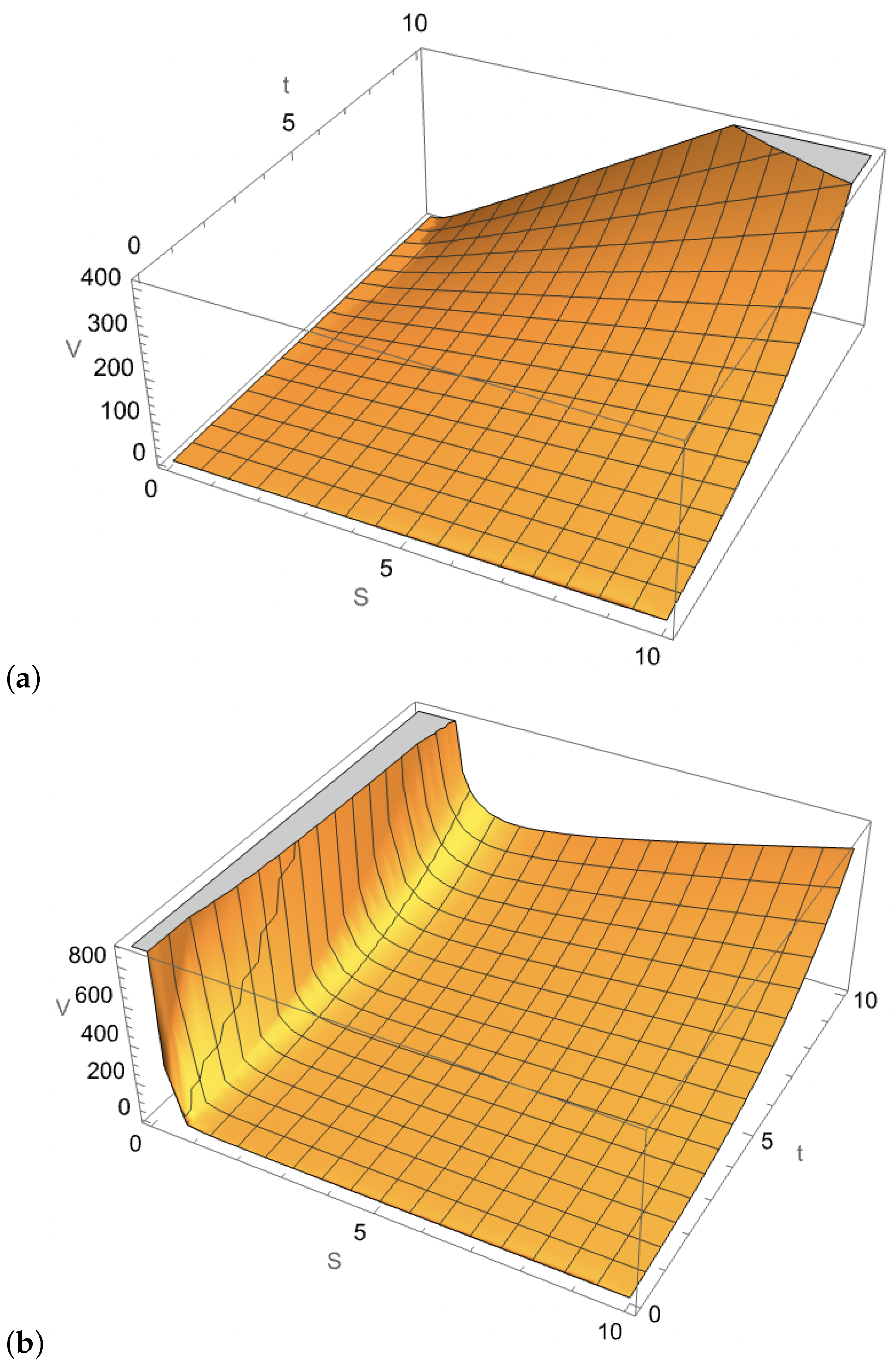
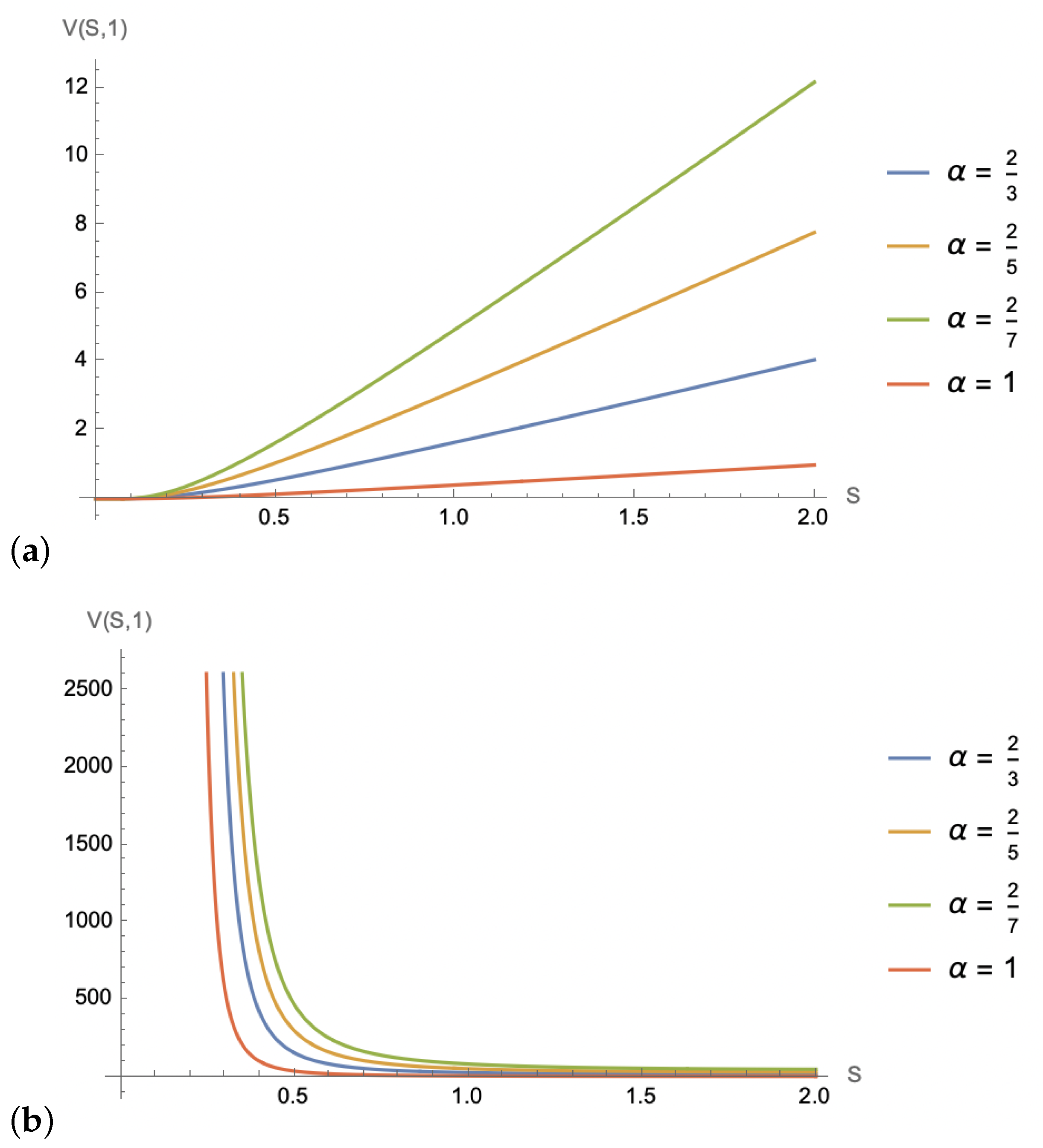
In Figure 1 and Figure 2, we showcase various graphical solutions from Theorem 3.

On the other hand, if we invoke the Caputo derivative of order $\alpha$, the solution of the general fractional pricing equation is given by the next theorem.

Theorem 4.

The general fractional pricing Equation (1), under a Caputo fractional derivative with $0<\alpha <1$, and parameters $\gamma =2,\kappa =\beta =0,\lambda =-\frac{1}{\rho }$, and ρ arbitrary, admits the invariant solution:

$$V(S,t)=-\frac{C\rho S}{\sqrt{2}}{E}_{\alpha }\left(\frac{b^2{\left(-t^{\alpha }\right)}^{\alpha }}{\Gamma (\alpha +1)}\right)exp\left(-\frac{\sqrt{2}b}{\rho S}+\frac{1}{{\rho }^{2}S}-\frac{{\left(-t^{\alpha }\right)}^{\alpha }}{2\alpha {\rho }^2\Gamma \left(\alpha \right)\Gamma (\alpha +1)}\right).$$

(26)

Proof. 

The proof is similar to that of Theorem 3; however, under the Caputo derivative of order $\alpha$, the solution of (19) is given by

$$\psi \left(\widehat{t}\right)=C{E}_{\alpha }\left(\frac{b^2}{\Gamma (\alpha +1)}{\widehat{t}}^{\alpha }\right),$$

(27)

where $E_{\alpha }$ is the classic Mittag-Leffler function defined as

$$E_{\alpha }\left(z\right)=\sum _{k=0}^{\infty }\frac{z^k}{\Gamma (\alpha k+1)},$$

(28)

with $\alpha >0.$ Therefore, from (18), we have

$$\omega (y,\widehat{t})=E_{\alpha }\left(\frac{b^2}{\Gamma (\alpha +1)}{\widehat{t}}^{\alpha }\right)e^{by},$$

(29)

which also solves Equation (11), and to obtain the solution $V(S,t)$ for the general bond pricing equation, we invoke the transformations from Theorem 1. □

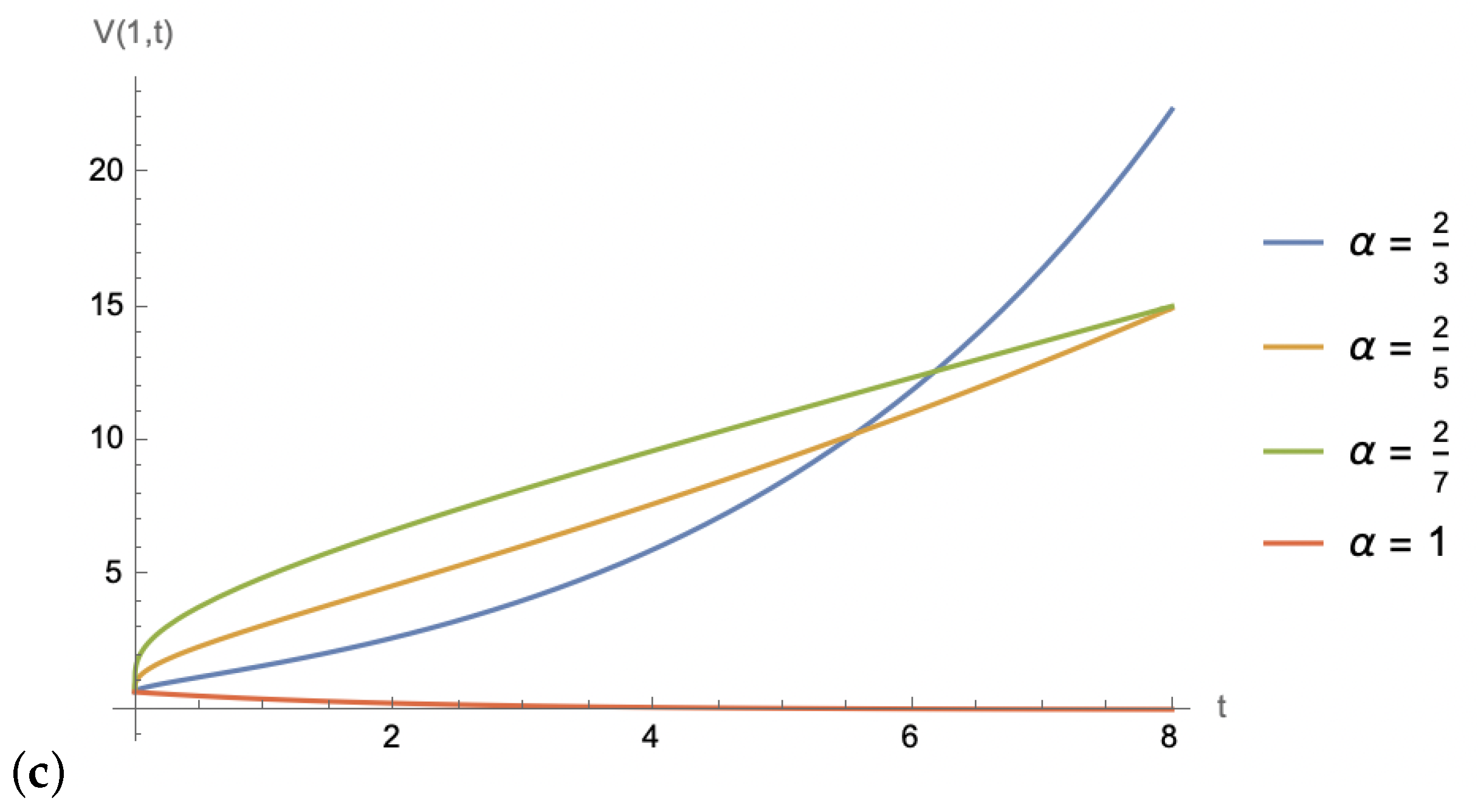
In Figure 3 and Figure 4, we showcase various graphical solutions from Theorem 4.

4. Results and Conclusions

The general pricing equation under study has had a major impact on the field of mathematical finance and the interpretation of financial instruments by serving as a foundation for a myriad of well-known models. These models arise from altering the market price of risk and other constant parameters, as such, there are more opportunities to develop and gain more insight through further experimentation. In this paper, we presented one such model and presented a way of arriving at solutions by leveraging the heat equation’s well-known symmetries and exploring the various definitions of fractional derivatives that the literature has to offer.

A study of Equation (1) resulted in two kinds of solutions for each fractional case, in addition to the standard integer derivative case. These solutions arise from the definition chosen to interpret the fractional derivative. The first is the Riemann–Liouville definition and the second is the Caputo fractional derivative. These derivatives are widely used in fractional calculus for various purposes and we have explored both for the potential solutions that they present. All of our results were collected via theorems and proofs.

Numerically, we note that the solutions via the Riemann–Liouville fractional derivative versus the Caputo fractional derivative are generally not the same. However, under both derivatives, the solutions behave similarly for $0<\alpha <1$ and $\alpha \to 1$. We observe a higher bond value, for variable time and fixed stock price, and a fractional derivative $0<\alpha <1$. That is, for $\alpha \to 1$ under those same conditions, we find lower bond values. Graphically, we also discover that the parameter b has a strong influence on the value of the bond, given a fixed time and variable stock price, with $b>0$ producing rapidly decaying values. This occurs due to the dominance of the time variable in the exponent’s argument. Overall, for sufficiently large values for the variables S and t, the solution $V(S,t)$ exhibits a similar behaviour of growth with the evolution of the variables and $b<0$. This model depicts a situation where the current value of the financial instrument is capable of growing over time. More importantly, given the restrictions on b, the dynamic of having the fractional derivative in the model implies improved bond values.

Mathematically, it is almost impossible to solve differential equations, especially those highly nonlinear and that possess higher-order derivatives, without the addition of a transformation—the branch of fractional equations is no different. Moreover, the goal of most transformations is to provide simpler versions of an original equation, such that tools from advanced calculus readily apply towards finding solutions. The transformation is a highly effective approach, and the only challenging element is to construct such transformations.

Our framework described above shows how important transformations are in fractional calculus. The above study further emphasises the compatibility of symmetry methods with fractional derivative models, especially for parameter selection in modelling scenarios.

References

- Zhang, W.-G.; Xiao, W.-L.; He, C.-X. Equity warrants pricing model under fractional Brownian motion and an empirical study. Expert Syst. Appl. 2009, 36, 3056–3065. [Google Scholar] [CrossRef]
- Garzarelli, F.; Cristelli, M.; Pompa, G.; Zaccaria, A.; Pietronero, L. Memory effects in stock price dynamics: Evidences of technical trading. Sci. Rep. 2014, 4, 4487. [Google Scholar] [CrossRef] [PubMed]
- Panas, E. Long memory and chaotic models of prices on the London metal exchange. Resour. Policy 2001, 4, 485–490. [Google Scholar] [CrossRef]
- Jumarie, G. Derivation and solutions of some fractional Black–Scholes equations in coarse-grained space and time. Application to Merton’s optimal portfolio. Comput. Math. Appl. 2010, 59, 1142–1164. [Google Scholar] [CrossRef]
- Liang, J.R.; Wang, J.; Zhang, W.J.; Qiu, W.Y.; Ren, F.Y. The solutions to a bi-fractional Black-Scholes-Merton differential equation. Int. J. Pure Appl. Math. 2010, 128, 99–112. [Google Scholar]
- Fall, A.N.; Ndiaye, S.N.; Sene, N. Black-Scholes option pricing equations described by the Caputo generalized fractional derivative. Chaos Solitons Fractals 2019, 125, 108–118. [Google Scholar] [CrossRef]
- Giona, M.; Roman, H.E. Fractional diffusion equation on fractals: One-dimensional case and asymptotic behaviour. J. Phys. A-Math. Gen. 1999, 25, 2093. [Google Scholar] [CrossRef]
- Yavuz, M.; Özdemir, N. European vanilla option pricing model of fractional order without singular kernel. Fractal Fract. 2018, 2, 3. [Google Scholar] [CrossRef]
- Wyss, W. The fractional Black-Scholes equation. Fract. Calc. Appl. Anal. 2000, 3, 51–61. [Google Scholar]
- Vasicek, O. An equilibrium characterization of the term structure. J. Financ. Econ. 1977, 5, 177–188. [Google Scholar] [CrossRef]
- Dothan, L. On the term structure of interest rates. J. Financ. Econ. 1978, 6, 59–69. [Google Scholar] [CrossRef]
- Cox, J.C.; Ingersoll, J.E.; Ross, S.A. An intertemporal general equilibrium model of asset prices. Econometrica 1985, 53, 363–384. [Google Scholar] [CrossRef]
- Brennan, M.J.; Schwartz, E.S. Analyzing convertible bonds. J. Financ. Quant. Anal. 1980, 15, 907–929. [Google Scholar] [CrossRef]
- Maphanga, R.; Jamal, S. A Terminal Condition in Linear Bond-Pricing under Symmetry Invariance. J. Nonlinear Math. Phys. 2023, 1–10. [Google Scholar] [CrossRef]
- Lie, S. Theorie der Transformationsgruppen I. Math. Ann. 1880, 16, 441–528. [Google Scholar] [CrossRef]
- Miller, K.S.; Ross, B. An Introduction to the Fractional Calculus and Fractional Differential Equations; Wiley: New York, NY, USA, 1993. [Google Scholar]
- Kiryakova, V. Generalised Fractional Calculus and Applications; Pitman Research Notes in Mathematics; Longman: London, UK, 1994; Volume 301. [Google Scholar]
- Podlubny, I. Fractional Differential Equations: An Introduction to Fractional Derivatives, Fractional Differential Equations, to Methods of Their Solution and Some of Their Applications; Academic Press: New York, NY, USA, 1998. [Google Scholar]
- Buckwar, E.; Luchko, Y. Invariance of a partial differential equation of fractional order under the Lie group of scaling transformations. J. Math. Anal. Appl. 1998, 227, 81–97. [Google Scholar] [CrossRef]
- Gazizov, R.K.; Kasatkin, A.A.; Lukashchuk, S.Y. Symmetry properties of fractional diffusion equations. Phys. Scr. 2009, T136, 014016. [Google Scholar] [CrossRef]
- Gazizov, R.K.; Kasatkin, A.A.; Lukashchuk, S.Y. Continuous transformation groups of fractional differential equations. Vestn. USATU 2007, 9, 125–135. [Google Scholar]
- Bakkyaraj, T. Lie symmetry analysis of system of nonlinear fractional partial differential equations with Caputo fractional derivative. Eur. Phys. J. Plus 2020, 135, 126. [Google Scholar] [CrossRef]
- Leo, R.A.; Sicuro, G.; Tempesta, P. A theorem on the existence of symmetries of fractional PDEs. C. R. Acad. Sci. Paris Ser. I 2014, 352, 219–222. [Google Scholar] [CrossRef]
- Sahadevan, R.; Bakkyaraj, T. Invariant analysis of time fractional generalized Burgers and Korteweg-de Vries equations. J. Math. Anal. Appl. 2012, 393, 341–347. [Google Scholar] [CrossRef]
- Kubayi, J.T.; Jamal, S. Lie Symmetries and Third- and Fifth-Order Time-Fractional Polynomial Evolution Equations. Fractal Fract. 2023, 7, 125. [Google Scholar] [CrossRef]
- Jamal, S. Imaging Noise Suppression: Fourth-Order Partial Differential Equations and Travelling Wave Solutions. Mathematics 2020, 8, 2019. [Google Scholar] [CrossRef]
- Obaidullah, U.; Jamal, S. A computational procedure for exact solutions of Burgers’ hierarchy of nonlinear partial differential equations. J. Appl. Math. Comput. 2020, 65, 541. [Google Scholar] [CrossRef]
- Yang, X.; Wu, L.; Zhang, H. A space-time spectral order sinc-collocation method for the fourth-order nonlocal heat model arising in viscoelasticity. Appl. Math. Comput. 2023, 457, 128192. [Google Scholar] [CrossRef]
- Kimeu, J.M. Fractional Calculus: Definition and Applications. Master’s Thesis, Western Kentucky University, Bowling Green, KY, USA, 2009. [Google Scholar]