Complex Dynamical Characteristics of the Fractional-Order Cellular Neural Network and Its DSP Implementation

Abstract

A new fractional-order cellular neural network (CNN) system is solved using the Adomian decomposition method (ADM) with the hyperbolic tangent activation function in this paper. The equilibrium point is analyzed in this CNN system. The dynamical behaviors are studied as well, using a phase diagram, bifurcation diagram, Lyapunov Exponent spectrum (LEs), and spectral entropy (SE) complexity algorithm. Changing the template parameters and the order values has an impact on the dynamical behaviors. The results indicate that rich dynamical properties exist in the system, such as hyperchaotic attractors, chaotic attractors, asymptotic periodic loops, complex coexisting attractors, and interesting state transition phenomena. In addition, the digital circuit implementation of this fractional-order CNN system is completed on a digital signal processing (DSP) platform, which proves the accuracy of ADM and the physical feasibility of the CNN system. The study in this paper offers a fundamental theory for the fractional-order CNN system as it applies to secure communication and image encryption.

1. Introduction

The study of biological neural networks is extremely significant to explore human brain thinking and intelligent activities. Artificial neural networks can simulate intelligent activities based on the working principles of the human brain to solve practical problems. Neural networks rely on the interaction of neurons to exhibit complex dynamical behaviors. Rich dynamical behaviors are found in a variety of neural networks and improved models [1,2,3,4,5]. It is worth mentioning that the full names of terminology corresponding to the abbreviations are shown in Table 1 for ease of reading and understanding the paper. The circuit structure called the cellular neural network (CNN) was proposed by Chua [6]. CNN enables real-time signals to be handled in parallel at high speed, and the structure can realize a Very Large-Scale Integration (VLSI) circuit due to local interconnectivity. Marco and Forti found that the complex dynamical properties occurred in a third-order CNN, which had a symmetric interconnection parameter matrix [7]. Meanwhile, many classes of systems based on the original CNN model have been designed, and hyperchaotic phenomena were found in certain systems [8,9,10,11,12]. In addition, different types of neural networks are extensively applied in diverse fields, including image processing, secure communications, and so on [13,14,15,16,17,18,19]. For example, Xiu et al. constructed a novel chaotic memristive CNN system, which is applied for secure communications through chaotic synchronization [13]. Norouzi et al. presented an improved approach to image encryption with high sensitivity depending on DNA sequence and CNN [18]. On the basis of a CNN hyperchaotic system, Zhang et al. put forward an image encryption scheme for achieving high security [19]. CNN has a broad and profound application prospect, but most studies of CNN are integer-order systems. There are a few studies about fractional-order CNN [20,21]. However, fractional-order systems can simulate CNN systems more accurately. Thus, this article concentrates on the construction and comprehensive analysis of fractional-order CNN systems.

Table 1. Full name corresponding to the abbreviation.

Full Name	Abbreviation
Cellular neural network	CNN
Adomian decomposition method	ADM
Lyapunov Exponent spectrum	LEs
Spectral entropy	SE
Digital signal processing	DSP
Frequency-domain method	FDM
Predictor-corrector method	PCM

The memory property and overall importance enable fractional calculus to be more accurate and efficient in describing models and dealing with problems [22,23,24,25,26,27,28,29]. Fractional-order chaotic systems can exhibit more abundant dynamical behaviors compared with integer-order systems. Meanwhile, the exact periodic solution does not exist in the fractional-order dynamical system, but the long-time periodic solution may exist in the fractional-order system [30]. In differential equations of fractional order, numerical solution algorithms are basic to theoretical analysis and practical application. To solve fractional-order chaotic systems, there are three common algorithms, which are the frequency-domain method (FDM) [31], predictor-corrector method(PCM) [32], and Adomian decomposition method (ADM) [33]. The FDM gives a basis in theory for fractional-order analog circuit implementation, but it does not take into account the historical information in the approximation process [34]. The PCM is a time domain analysis algorithm in which the order of the differential operator can calculate smaller steps. However, this method requires more operation time and memory space since each iteration uses all the previous data. The ADM is suitable for digital circuit implementation, which has been widely applied to various fractional-order neural networks owing to its more accurate numerical solutions and faster convergence [35,36,37]. Jahanshahi et al. studied dynamical behaviors and synchronization in a fractional-order Hopfield-like neural network [38]. Huang et al. came up with a four-cell fractional order CNN and found rich dynamical behaviors [39]. Therefore, the ADM is used for solving the fractional-order CNN system accurately in this paper.

The nonlinear activation function is the center of neural networks. Between layers of a neural network, the activation function is adapted to output values of the former layer in a tolerable range to input values of the latter. The option of activation function can have a huge effect on enhancing the efficiency and performance of neural networks [40]. Associative memory can be achieved through equilibrium point stability in CNN, Han et al. used thresholding activation to study equilibrium points of CNN in different parameter regions [41]. Masahiro Nakagawa proposed Chebyshev-type functions to act as activation functions in the chaos neuron models [42]. Different types of activation functions have different characteristics and apply to various classes of neural networks [43,44,45]. The hyperbolic tangent function has some similar properties to the segmented linear function in the previous CNN. Further, its ideal steep derivative improves the efficiency of fast learning [46,47]. Meanwhile, the smooth mathematical nature of the hyperbolic tangent function makes it easier to complete hardware design and implementation than the initial segmented linear function. Therefore, the hyperbolic tangent function is utilized as an activation function of the fractional-order CNN system. Furthermore, this system is implemented using DSP for proving its physical feasibility. And it provides the digital circuit foundation for practical application research based on the system.

Based on the above issues, this paper proposes a novel fractional-order cellular neural network (CNN) system based on a hyperbolic tangent activation function and solves the system using the Adomian decomposition method (ADM). The ideal steep derivative of the hyperbolic tangent activation function improves the efficiency of the previous CNN. Various analytical approaches indicate the presence of rich dynamical behaviors in the system, including diverse attractors, attractor coexistence, and state transition phenomena.

The rest of the manuscript is organized as follows. Section 2 demonstrates the construction of the fractional-order CNN system with an activation function tanh and presents its solution process of ADM. In Section 3, the stability of equilibrium points is analyzed. The influences of the order and system parameters on the dynamical behaviors are also studied. The complex dynamical characteristics of the system are investigated. Section 4 displays the DSP implementation. Lastly, some conclusions are obtained.

2. CNN System with Hyperbolic Tangent Activation Function

2.1. Adomian Decomposition Method

The ADM is broadly accepted for solving linear and nonlinear differential equations which was proposed by Adomian. This approach can be applied to solving fractional-order systems. The fractional-order system is represented as

$$\{\begin{array}{l}\ast D_{t_0}^{q}x(t)=Lx+Nx+g(t)\\ x^{(k)}(t_0^{+})=b_k,k=0,1,\cdots ,n-1\\ n\in N,n-1<q\le n\end{array},$$

(1)

where *$D_t^q$₀means Caputo differential operation about order q, b_k means initial value. The system equation generally consists of three parts: linear L, nonlinear N, and constant g(t). After the integration of two sides in Equation (1), the result can be obtained as

$$\{\begin{array}{l}x=J_{t_0}^{q}Lx+J_{t_0}^{q}Nx+J_{t_0}^{q}g+\phi \\ \phi ={\displaystyle \sum _{k=0}^{m-1}{b}_k\frac{{(t-t_0)}^k}{k!}}\end{array},$$

(2)

where $J_t^q$₀ refers to the Riemann–Liouville integral operator, φ is the initial value condition. $J_{t_0}^q$ integral calculation fulfills below fundamental properties

$$\{\begin{array}{l}{J}_{t_0}^q{(t-t_0)}^{\gamma }=\frac{\Gamma (\gamma +1)}{\Gamma (\gamma +1+q)}{(t-t_0)}^{\gamma +q}\\ J_{t_0}^{q}C=\frac{C}{\Gamma (q+1)}{(t-t_0)}^q\\ J_{t_0}^q{J}_{t_0}^{r}x(t)=J_{t_0}^{q+r}x(t)\end{array}.$$

(3)

According to the ADM algorithm, the nonlinear part is decomposed into an equivalent special polynomial through the following equation

$$\{\begin{array}{l}{A}_j^i=\frac{1}{i!}{\left[\frac{d^{i}N(v_j^i(\lambda ))}{d{\lambda }^i}\right]}_{\lambda =0}\\ v_j^i(\lambda )={\displaystyle \sum _{k=0}^i{(\lambda )}^k{x}_j^k}\end{array},i=0,1,2\dots \infty ;j=1,2\dots \infty .$$

(4)

The nonlinear polynomial is given as

$$Nx={\displaystyle \sum _{i=0}^{\infty }{A}^i}(x^0,x^1,\cdots ,x^i).$$

(5)

Therefore, the solution of the fractional order system then is expressed as

$$x={\displaystyle \sum _{i=0}^{\infty }{x}^i}=J_{t_0}^{q}L{\displaystyle \sum _{i=0}^{\infty }{x}^i+J_{t_0}^{q}N{\displaystyle \sum _{i=0}^{\infty }{A}^i+J_{t_0}^{q}g+\phi }}.$$

(6)

The solution components can be further indicated as

$$\{\begin{array}{c}{x}^0=\phi \hfill \\ x^1=J_{t_0}^{q}L{x}^0+J_{t_0}^q{A}^0(x^0)\hfill \\ \dots \\ x^i=J_{t_0}^{q}L{x}^{i-1}+J_{t_0}^q{A}^{i-1}(x^0,x^1,\dots ,x^{i-1})\hfill \\ \dots \end{array}.$$

(7)

2.2. Solution of the Fractional-Order CNN System

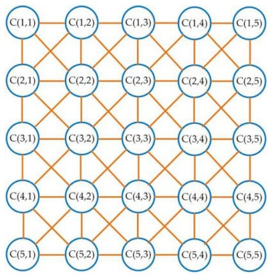
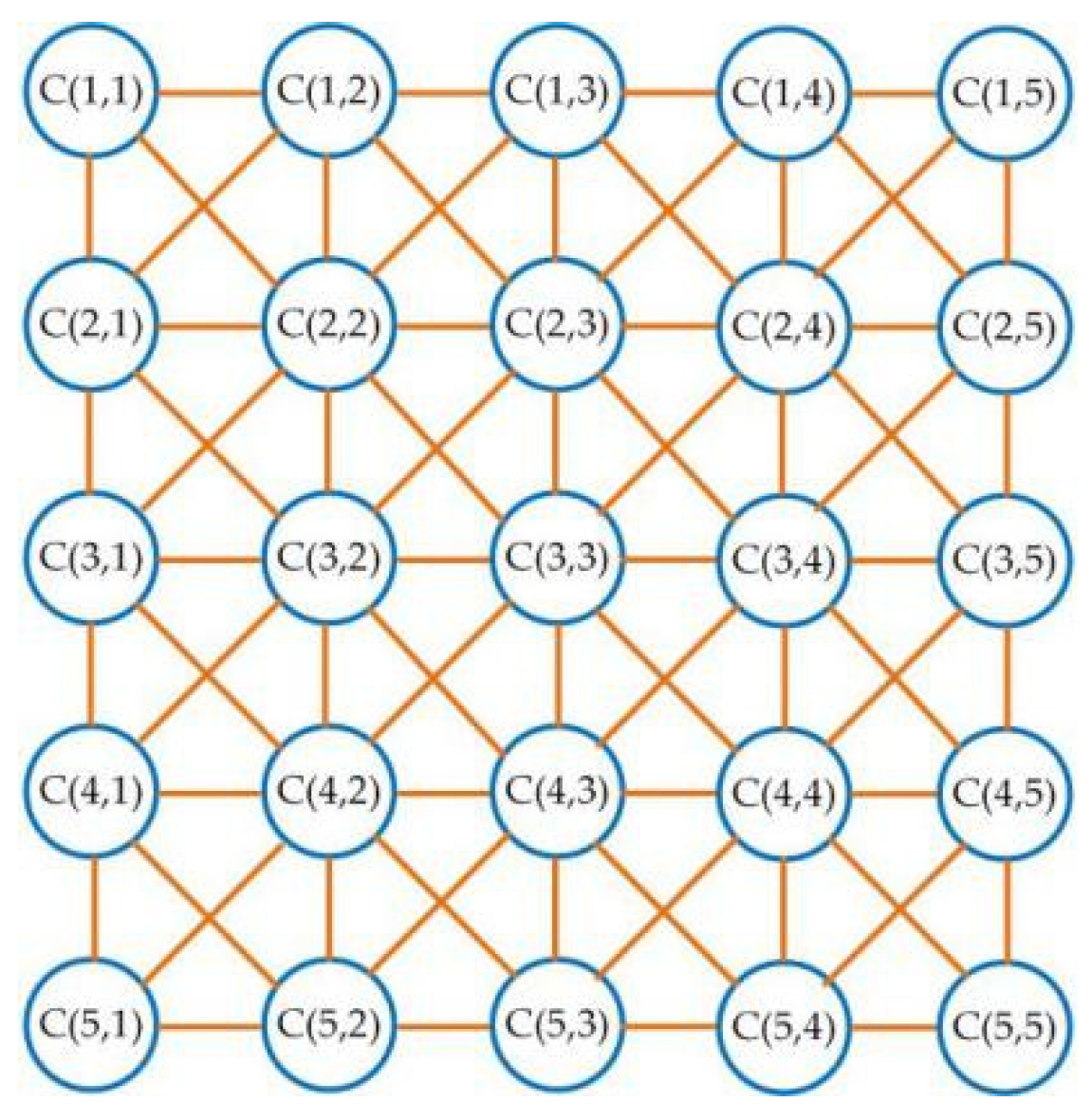
The CNN is an effective and flexible circuit structure, but it owns the essential features of biological neural networks. CNNs can be viewed as multiple basic cellular circuits connected in a neighborhood connection mode. The basic circuit is described as a cell. When the cells are organized in u rows and v columns, the cell located in row i and column j can be expressed as C(i, j). The simple CNN structure with two-dimensional arrangement and 5 × 5 size is given in Figure 1, and its neighborhood value r = 2. The definition of r-neighborhood is

$$N_r(i,j)=\{C(k,l)|\max \{|k-i|,|k-i|\}\le r,1\le k\le u;1\le k\le v\}.$$

(8)

Figure 1. The construction of a two-dimensional 5 × 5 CNN.

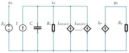
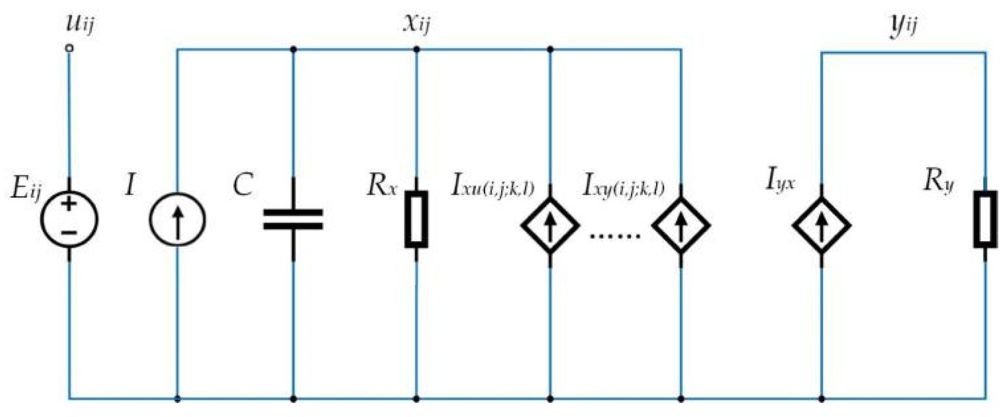
The circuit architecture of each detailed cell is depicted in Figure 2. Each cell has one capacitor C, two resistors Rx, Ry, and several linear voltage control current sources coupled to neighbor cells. The u_ij, y_ij, and x_ij denote the input, output, and state variables separately. E_ij and I refer to independent voltage and current source, respectively. As the single nonlinear component, I_yx is a segmented linear voltage-controlled current source in a unit.

Figure 2. A detailed cell circuit structure for CNN.

The circuit state equation of a cell is

$$c\frac{d{x}_{ij}(t)}{dt}=-\frac{x_{ij}(t)}{R_x}+{\displaystyle \sum _{C(k,l)\in {{\rm N}}_r(i,j)}{A}_{(i,j;k,l)}{y}_{kl}(t)}+{\displaystyle \sum _{C(k,l)\in {{\rm N}}_r(i,j)}{B}_{(i,j;k,l)}{u}_{kl}(t)+I},$$

(9)

where

$$I_{xy(i,j;k,l)}=A_{(i,j;k,l)}{y}_{kl}(t),I_{xu(i,j;k,l)}=B_{(i,j;k,l)}{u}_{kl}(t).$$

(10)

In Equation (10), A_(i,j;k,l) is called an interactive parameter. And it affects the output feedback of CNN. B_(i,j;k,l) is the control parameter, which has an impact on the input control effect of CNN.

The output equation in the CNN unit circuit is

$$y_{kl}(t)=\frac{1}{2}(|x_{ij}(t)+1|-|x_{ij}(t)-1|).$$

(11)

The output equation affects I_xy(i,j;k,l) as presented in Equation (10), and it can be viewed as the activation function of CNN. The activation function controlling neuron output affects the properties of the neuron in the neural network. Neural networks can be used with multiple types of activation functions. The hyperbolic tangent function tanh(x) has a fast convergence rate. The zero mean property of function tanh brings the artificial neural network even closer to the biological state. In practice, the tanh(x) function can be used for better sparsity. Compared with the original segmented linear function, the smooth mathematical property of the hyperbolic tangent function is easier to design and implement in hardware. The function tanh(x) is used as the activation function in this system due to its advantages. Therefore, the segmented linear output equation y_kl(t) in the original CNN cell circuit is replaced by

$$y_{kl}(t)=\tan \mathrm{h}(x_{ij}(t)).$$

(12)

The forms of simplified models of CNN are various. To make research more convenient, a simplified equation model of a fully interconnected CNN system is introduced as follows

$$\frac{d{x}_j}{dt}=-x_j+p_j{y}_k(t)+{\displaystyle \sum _{k=1,k\ne j}^5{A}_{jk}{y}_k(t)}+{\displaystyle \sum _{k=1}^5{S}_{jk}{x}_k+I_j},j=1,2,3,4,5,$$

(13)

where x_j and y_k, refer to the state variable and output, A_jky_k(t) and S_jkx_k represent the output and state variable in connected cells, I_j represents the bias current. Based on three generalized cells models [48] and lots of experiments with coefficients, the appropriate coefficients are chosen.

Setting P_j = 0(j ≠ 0), P₄ = b, I_j = 0, A_jk = 0,

$$S_{jk}=\left[\begin{array}{ccccc}1& 0& -1& -1& 0\\ 0& 3& 1& 0& 0\\ 12& -a& 1& 0& 0\\ 96& 0& 0& -89& 0\\ 0& 0& 15& 0& -1\end{array}\right],$$

(14)

the differential equation for the fractional-order CNN system is denoted in

$$\{\begin{array}{l}\ast D_{t_0}^q{x}_1(t)=-x_3-x_4\\ \ast D_{t_0}^q{x}_2(t)=2x_2+x_3\\ \ast D_{t_0}^q{x}_3(t)=12x_1-a{x}_2\\ \ast D_{t_0}^q{x}_4(t)=96x_1-90x_4+b\tanh (x_4)\\ \ast D_{t_0}^q{x}_5(t)=15x_3-2x_5\end{array}.$$

(15)

According to Equation (6), the linear and nonlinear terms can be decomposed into

$$\left[\begin{array}{l}L{x}_1\\ L{x}_2\\ L{x}_3\\ L{x}_4\\ L{x}_5\end{array}\right]=\left[\begin{array}{l}-x_3-x_4\\ 2x_2+x_3\\ 12x_1-a{x}_2\\ 96x_1-90x_4\\ 15x_3-2x_5\end{array}\right],\left[\begin{array}{l}N{x}_1\\ N{x}_2\\ N{x}_3\\ N{x}_4\\ N{x}_5\end{array}\right]=\left[\begin{array}{l}0\\ 0\\ 0\\ b\tanh (x_4)\\ 0\end{array}\right],\left[\begin{array}{l}{g}_1\\ g_2\\ g_3\\ g_4\\ g_5\end{array}\right]=\left[\begin{array}{l}0\\ 0\\ 0\\ 0\\ 0\end{array}\right].$$

(16)

It is clear that the nonlinear term of the system has only one hyperbolic tangent function tanh(x₄). The nonlinear term tanh(x₄) is decomposed in accordance with Equation (4) as follows

$$\begin{array}{ll}{A}_4^0& =\tanh (x_4^0)\\ A_4^1& =x_4^1{\mathrm{sech}}^2(x_4^0)\\ A_4^2& =x_4^2{\mathrm{sech}}^2(x_4^0)-{(x_4^1)}^2{\mathrm{sech}}^2(x_4^0)\tanh (x_4^0).\\ A_4^3& =x_4^3{\mathrm{sech}}^2(x_4^0)-2x_4^2{x}_4^1{\mathrm{sech}}^2(x_4^0)\tanh (x_4^0)\\ & +\frac{1}{3}(x_4^1{)}^3(4{\mathrm{sech}}^3(x_4^0){\tanh }^2(x_4^0)-{\mathrm{sech}}^4(x_4^0))\end{array}$$

(17)

In this system, the initial value can be defined as

$$\{\begin{array}{l}{x}_1^0=x_1(t_0)\\ x_2^0=x_2(t_0)\\ x_3^0=x_3(t_0)\\ x_4^0=x_4(t_0)\\ x_5^0=x_5(t_0)\end{array}.$$

(18)

Setting $c_1^0$= $x_1^0$, c0 2 = $x_2^0$, c0 3 = $x_3^0$, c0 4 = $x_4^0$, c0 5 = $x_5^0$, according to the integral properties Equation (3), the second state variable can be denoted as

$$\{\begin{array}{l}{x}_1^1=(-c_3^0-c_4^0)\frac{{(t-t_0)}^q}{\Gamma (q+1)}\\ x_2^1=(2c_2^0+c_3^0)\frac{{(t-t_0)}^q}{\Gamma (q+1)}\\ x_3^1=(12c_1^0-a{c}_2^0)\frac{{(t-t_0)}^q}{\Gamma (q+1)}.\\ x_4^1=(96c_1^0-90c_4^0+b\tanh (c_4^0))\frac{{(t-t_0)}^q}{\Gamma (q+1)}\\ x_5^1=(15c_3^0-2c_5^0)\frac{{(t-t_0)}^q}{\Gamma (q+1)}\end{array}$$

(19)

And then assign the coefficient to the relevant variable, obtaining

$$\{\begin{array}{l}{c}_1^1=-c_3^0-c_4^0\\ c_2^1=2c_2^0+c_3^0\\ c_3^1=12c_1^0-a{c}_2^0.\\ c_4^1=96c_1^0-90c_4^0+b\tanh (c_4^0)\\ c_5^1=15c_3^0-2c_5^0\end{array}$$

(20)

It is obvious that x¹ can be expressed as c¹(t − t₀)/r(q + 1). The coefficients corresponding to other terms also can be solved in the same way. The results are presented in Appendix A.

Eventually, the approximate solution of the CNN fractional-order system is represented as

$${\tilde{x}}_j(t)=c_j^0+c_j^1\frac{{(t-t_0)}^q}{\Gamma (q+1)}+c_j^2\frac{{(t-t_0)}^q}{\Gamma (2q+1)}+c_j^3\frac{{(t-t_0)}^q}{\Gamma (3q+1)}+c_j^4\frac{{(t-t_0)}^q}{\Gamma (4q+1)},$$

(21)

where j = 1, 2, 3, 4, 5.

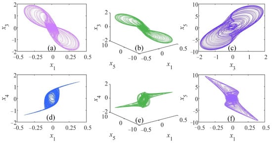
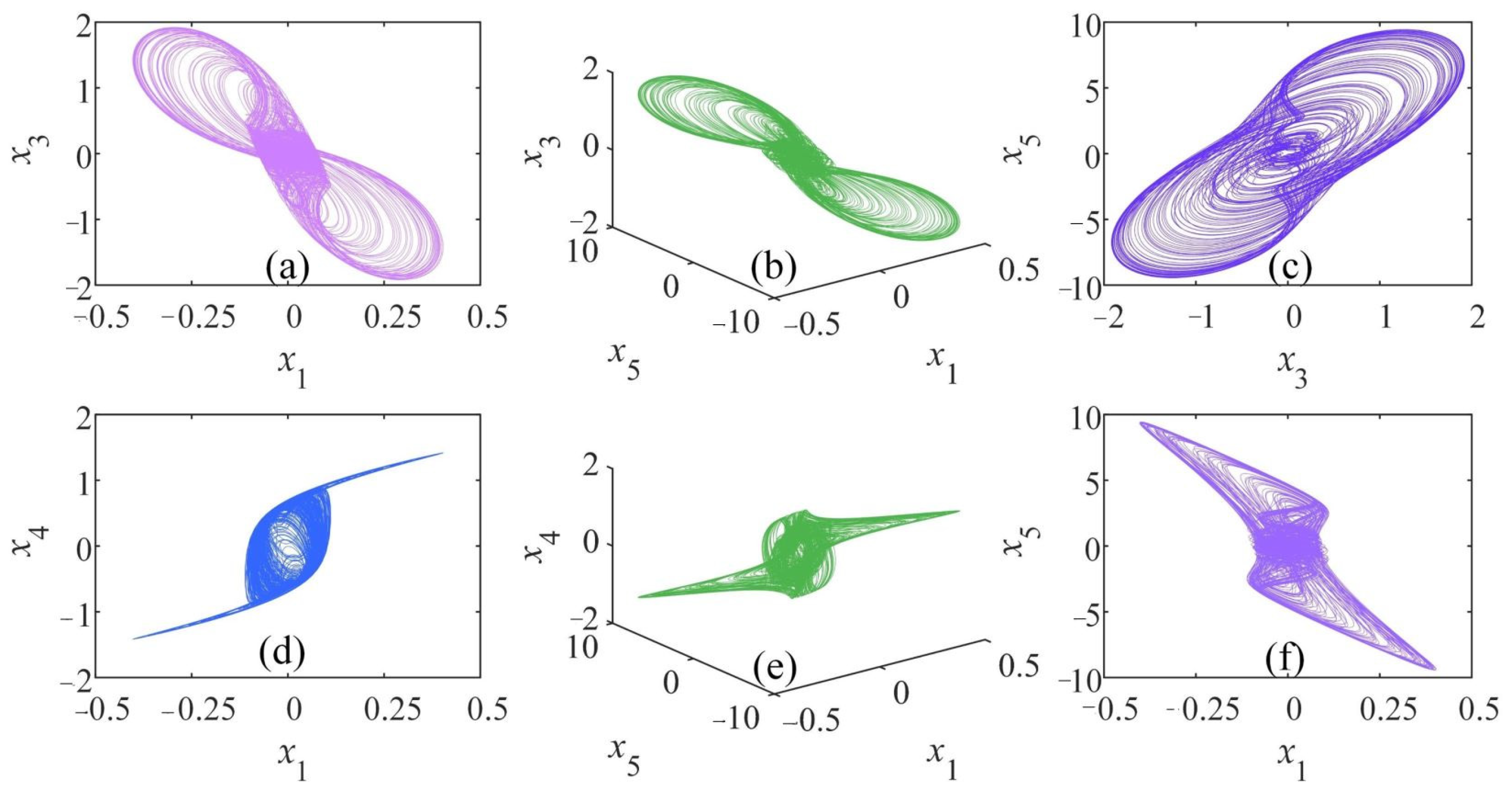
During the above iterative calculation, the entire interval is segmented into subintervals with an iteration step of h. Meanwhile, the values acquired in the former subinterval are regarded as initial values of the next subinterval. In this paper, the computer with a 64-bit win10 operating system and Intel(R) Core(TM) i7-8550U CPU @1.80 GHz processor is used for the experiment. The system solution and analysis are carried out on the MATLAB platform, version R2018a. Setting h = 0.01, a = 7, b = 100, q = 0.86, and initial values x₀ = (0.1, 0.01, 0.1, 1, 0.1). The Lyapunov exponents of the CNN system are L₁ = 1.3400, L₂ = 0, L₃ = −1.6721, L₄ = −6.2974, L₅ = −80.6484. With one positive Lyapunov exponent, the CNN system can generate the chaotic attractor as its phase diagram is shown in Figure 3.

Figure 3. Phase diagrams of chaotic attractor with a = 7, b = 100, q = 0.86: (a) x₁ − x₃ plane; (b) x₁ − x₅ − x₃ plane; (c) x₃ − x₅ plane; (d) x₁ − x₄ plane; (e) x₁ − x₅ − x₄ plane; (f) x₁ − x₅ plane.

3. Analysis of Dynamical Characteristics of the CNN System

3.1. Stability of Equilibrium Points

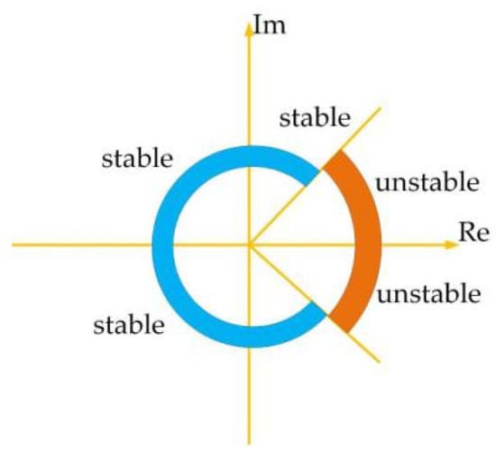
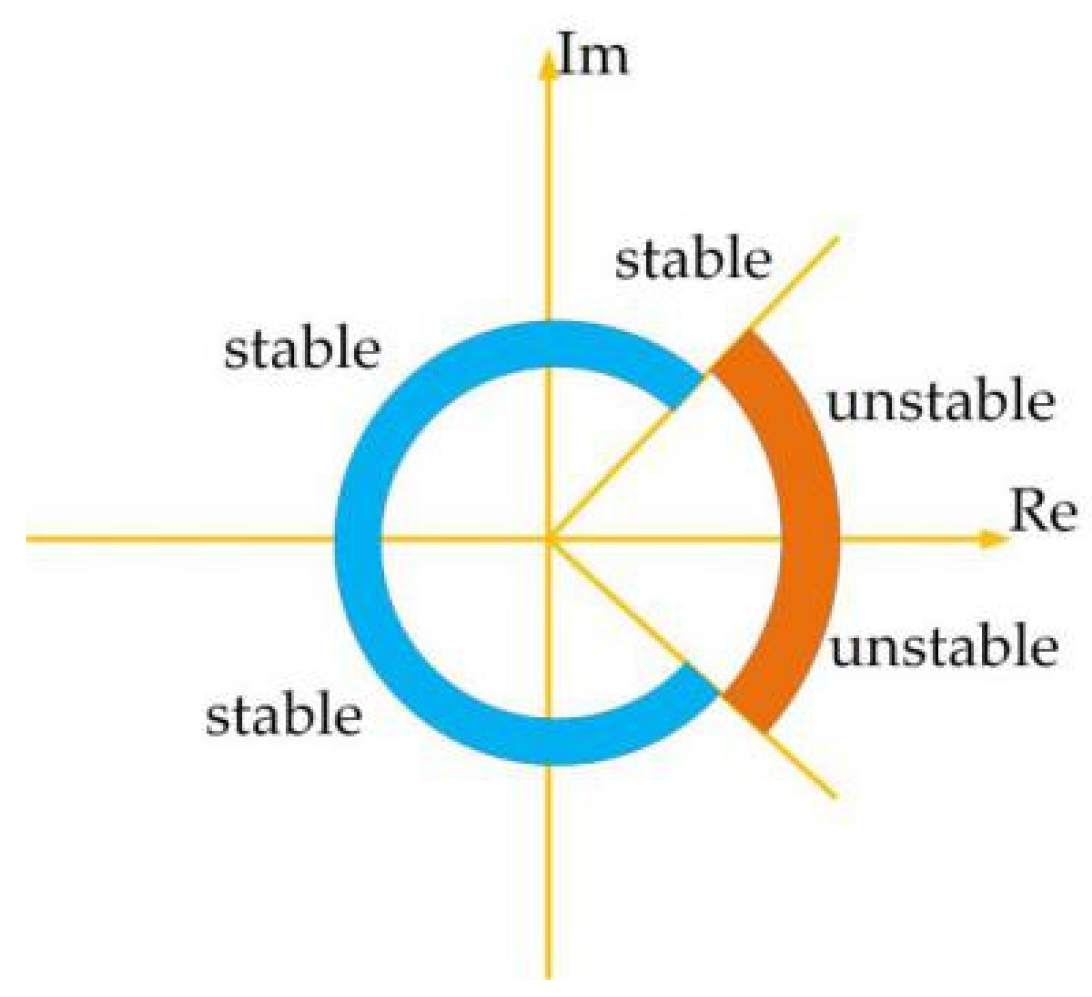
In high-dimensional dynamical systems, the stability of equilibrium points is related to the eigenvalues character of the Jacobian matrix. Remarkably, unlike the integer system, the fractional-order system is stable when its Jacobian eigenvalues satisfied Equation (22). According to the characteristics of the equilibrium point eigenvalues, the stability of equilibrium points can be easily determined. The stable region is a sector of a complex plane in normal fractional-order systems, and the stability distribution is shown in Figure 4.

$$\arg (\lambda )\ge \frac{\pi \alpha }{2},\alpha =\max (q_j,j=1,2,3,4,5).$$

(22)

Figure 4. Stability region of fractional-order systems.

To acquire equilibrium points, let

$$\{\begin{array}{l}-x_3-x_4=0\\ 2x_2+x_3=0\\ 12x_1-a{x}_2=0.\\ 96x_1-90x_4+b\tanh (x_4)=0\\ 15x_3-2x_5=0\end{array}$$

(23)

After calculating, whatever the value of a and b, the equilibrium point, which is the original point O(0, 0, 0, 0, 0) must exist in this system. The Jacobian matrix of the CNN system is

$$J=\left[\begin{array}{ccccc}0& 0& -1& -1& 0\\ 0& 2& 1& 0& 0\\ 12& -a& 0& 0& 0\\ 96& 0& 0& -90+b{\mathrm{sech}}^2(x_4)& 0\\ 0& 0& 15& 0& -2\end{array}\right].$$

(24)

The equilibrium point situation is various for different system parameter values. For example, when a = 7, the characteristic function of the system equilibrium point is denoted as

$$\begin{array}{l}{\lambda }^5+(90-b{\mathrm{sech}}^2(x_4)){\lambda }^4+111{\lambda }^3+(1364-15b{\mathrm{sech}}^2(x_4)){\lambda }^2\\ +(1500-14b{\mathrm{sech}}^2(x_4))\lambda +48b{\mathrm{sech}}^2(x_4)-2976=0\end{array}$$

(25)

$$\begin{array}{l}90-b{\mathrm{sech}}^2(x_4)>0.1364-15b{\mathrm{sech}}^2(x_4)>0\\ 1500-14b{\mathrm{sech}}^2(x_4)>0.48b{\mathrm{sech}}^2(x_4)-2976>0\end{array}$$

(26)

According to the Routh–Hurwitz rule, the system is stable as terms in Equation (26) are met. Due to 0 ≤ sech²(x₄) ≤ 1, it can be clearly known if b < 107.14, the characteristic function of the system is a positive real root. When q ∈ [0, 1], the corresponding equilibrium point is an instable saddle point. Keeping the parameter value a to 7, the equilibrium point characteristics are analyzed as b = 100 and b = 90, respectively. When b = 100, the equilibrium points are obtained in Equation (27) with relevant eigenvalues listed in Equation (28).

$$\{\begin{array}{l}{X}_{p0}={[0,0,0,0,0]}^{\mathrm{T}}\\ X_{p1}={[0.4206,0.7211,-1.4421,1.4421,-10.8161]}^{\mathrm{T}}\\ X_{p2}={[-0.4206,-0.7211,1.4421,-1.4421,10.8161]}^{\mathrm{T}}\end{array}.$$

(27)

$$\{\begin{array}{l}{X}_0:-2,1.6804\pm 2.5740i,4.3196\pm 8.8237i\\ X_1:-2,0.8797,-68.5481,-0.1383\pm 4.0835i\\ X_2:-2,0.8797,-68.5481,-0.1383\pm 4.0835i\end{array}.$$

(28)

According to Equation (22), equilibrium X_p0 is a stable point as q ≤ 0.7101. Meanwhile, the equilibrium X_p1 and X_p2 are unstable saddle points and |arg(λ₄)| = 1.5369.

In the same way, when b = 90, the equilibrium points are solved in Equation (29) and the corresponding eigenvalues are calculated in Equation (30).

$$\{\begin{array}{l}{X}_{p0}={[0,0,0,0,0]}^{\mathrm{T}}\\ X_{p1}={[0.3553,0.6090,-1.2180,1.2180,-9.1349]}^{\mathrm{T}}\\ X_{p2}={[-0.3553,-0.6090,1.2180,-1.2180,9.1349]}^{\mathrm{T}}\end{array}.$$

(29)

$$\{\begin{array}{l}{X}_0:-2,0.99232\pm 2.27863i,0.00771\pm 10.43038i\\ X_1:-2,0.83122,-61.81427,-0.18972\pm 4.05989i\\ X_2:-2,0.83122,-61.81427,-0.18972\pm 4.05989i\end{array}.$$

(30)

The results show that the equilibrium X_p1 and X_p2 are unstable saddle points in this fractional-order CNN system. The saddle point is the key to generating chaotic attractors. The above method can be used to analyze the equilibrium point when the template parameters are set to other values.

3.2. Influence of Different System Parameters

3.2.1. Influence of the Order q

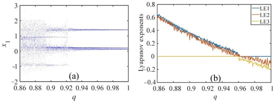
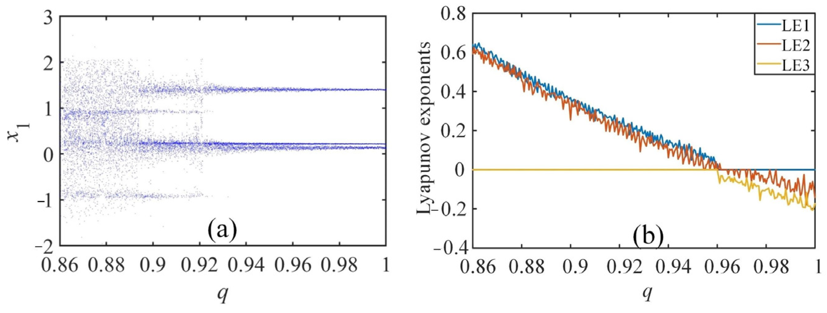
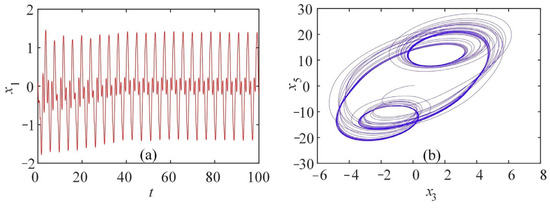
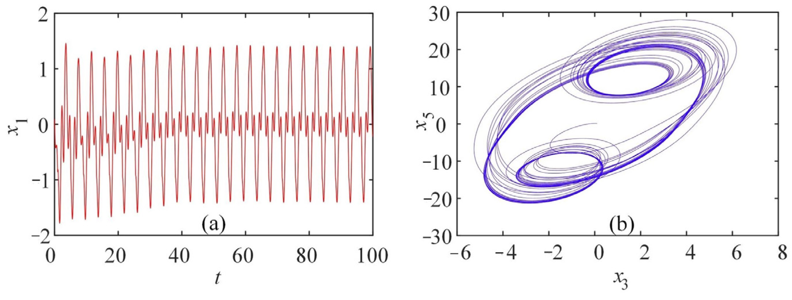
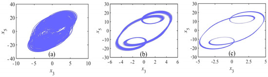
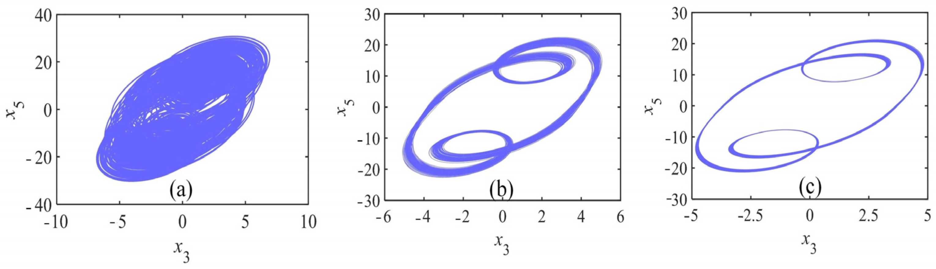
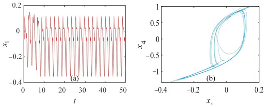
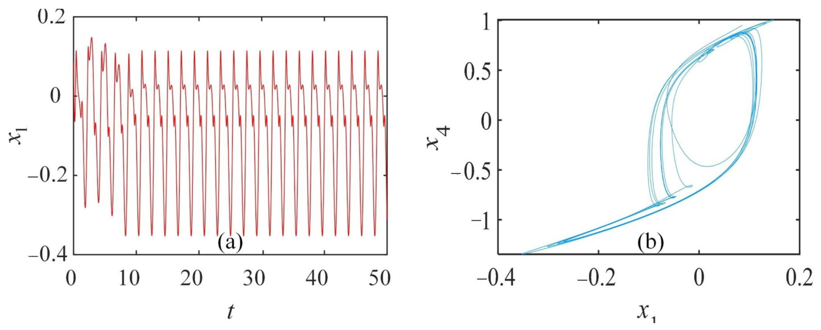
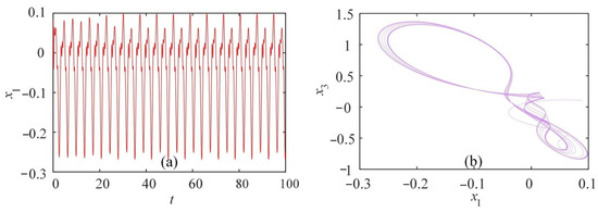
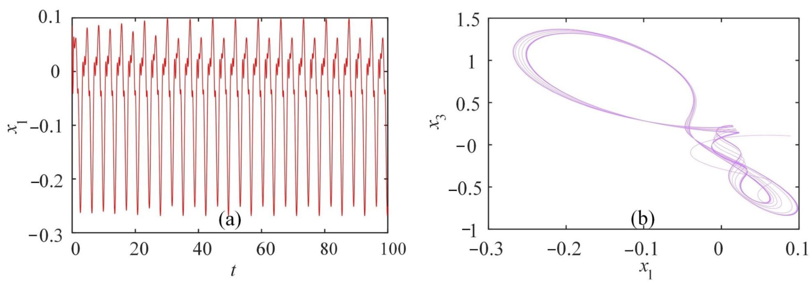
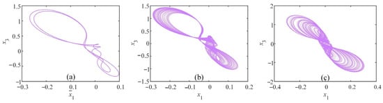
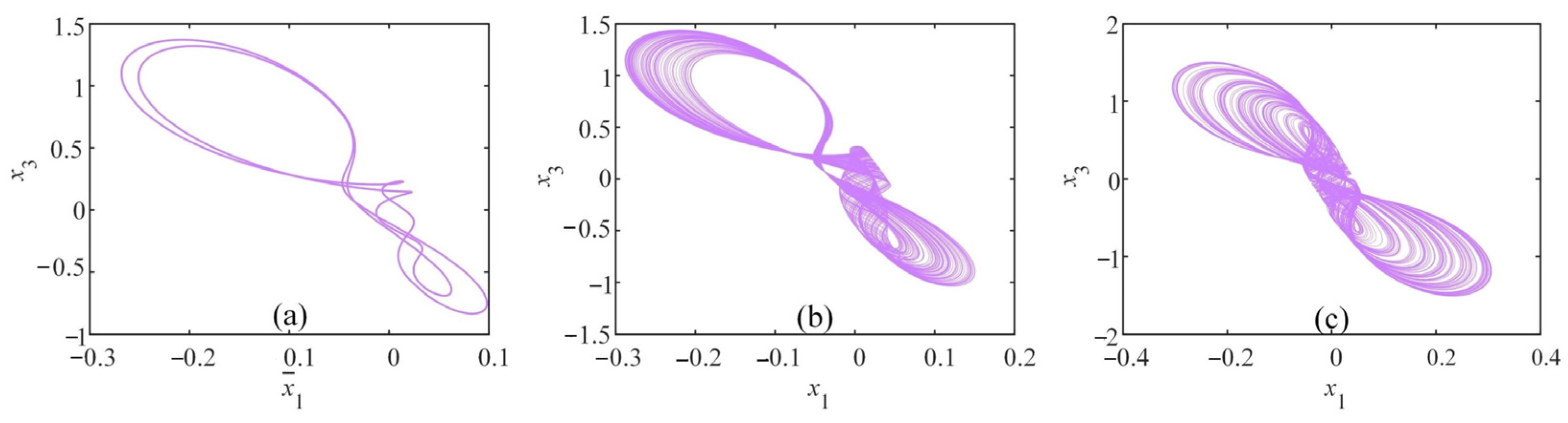
Some methods are used to study the dynamical characteristics of this system on the MATLAB R2018a platform. With q at a range of [0.86, 1], setting parameter a = 12, b = 201, initial values x₀ = (1, 0.1, 1, 1, 0.1), the bifurcation diagram along with the corresponding Lyapunov exponential spectrum are consistently depicted in Figure 5. The fourth and fifth Lyapunov exponents of the system are small negative numbers, which are hidden in the following analysis for showing more clearly how Lyapunov exponents vary with the order and parameters. As q ∈ [0.86, 0.96], the system is hyperchaotic since possessing two positive Lyapunov exponents. In particular, the fractional-order differential equation cannot exist in an exact periodic solution. When q ∈ [0.96, 1], the CNN fractional order system converts to an asymptotic periodic state. For example, when q = 0.98, the system converges an asymptotic periodic attractor in Figure 6b. The time series represents the asymptotic periodic solution of the system time in Figure 6a. However, the long-time solution is periodic in the system after 40 s. To clearly observe the system state, the various attractors selecting different order q are presented in Figure 7. The asymptotic periodic attractor in Figure 7 is the orbit corresponding to the long-time solution. As the order q becomes larger, the attractor gradually changes from a hyperchaotic attractor to an asymptotic periodic loop in a long-time mode.

Figure 5. Dynamical behavior with q ∈ [0.86, 1], a = 12, b = 201: (a) Bifurcation diagram; (b) LEs.

Figure 6. Asymptotic periodic behavior with q = 0.98: (a) Time sequences; (b) Phase diagram of the asymptotic periodic attractor.

Figure 7. Phase diagrams with a = 12, b = 201: (a) x₃ − x₅ plane as q = 0.89; (b) x₃ −x₅ plane as q = 0.93; (c) x₃ − x₅ plane as q = 0.98.

3.2.2. Influence of the Parameter a

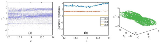
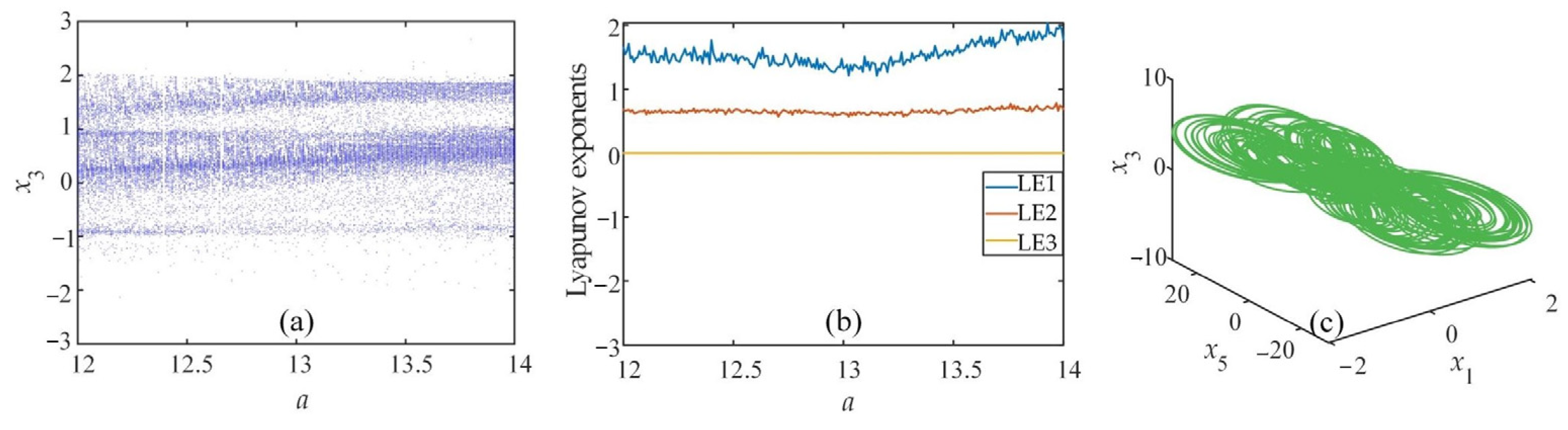
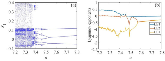
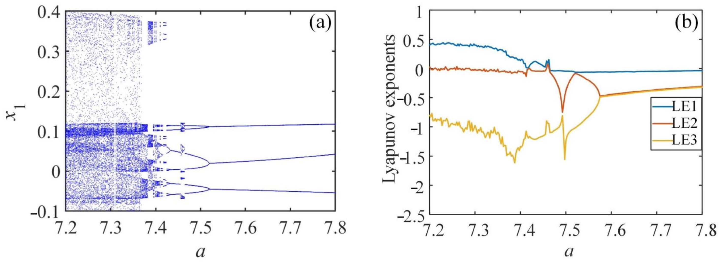
The template parameters have a certain influence on the dynamical properties of the system as well. According to Figure 8, when the order q = 0.88, parameter b = 200, initial values x₀ = (1, 0.1, 1, 1, 0.1), the system is in a global hyperchaotic state as the range of a is [12, 14]. Moreover, fixing the order q = 0.95, parameter b = 100, initial values x₀ = (0.1, 0.01, 0.1, 1, 0.1), as a varies from 7.2 to 7.8, the bifurcation diagram along with Lyapunov exponential spectrum is displayed in Figure 9. The system is first chaotic with a ∈ (7.2, 7.36). When a = 7.36, the bifurcation area jumps unsteadily. Afterwards, the system turns into an asymptotic periodic state from a = 7.46 through reverse-period-doubling bifurcation. When a = 7.65, the time sequences and asymptotic periodic attractor are presented in Figure 10. As a increases, the system state transforms from chaotic to asymptotic periodic in a long-time pattern. For clearly studying dynamical behaviors, the attractor trajectory is depicted in Figure 11 as a varies. The attractor types corresponding to different parameters a are shown in Table 2.

Figure 8. Hyperchaotic behavior with a ∈ [12, 14], q = 0.88, b = 200: (a) Bifurcation diagram; (b) LEs; (c) x₁ − x₅ − x₃ plane when a = 12.

Figure 9. Dynamical behavior with a ∈ [7.2, 7.8], q = 0.95, b = 100: (a) Bifurcation diagram; (b) LEs.

Figure 10. Asymptotic periodic behavior with a = 7.65: (a) Time sequences; (b) Phase diagram of the asymptotic periodic attractor.

Figure 11. Phase diagrams with q = 0.95, b = 100: (a) Chaos-I, a = 7.25; (b) Asymptotic Period-II, a = 7.48; (c) Asymptotic Period-I, a = 7.65.

Table 2. System state of different parameter a in a long-time pattern when q = 0.95, b = 100.

a	System State	a	System State
[7.2, 7.36]	Chaos-I	[7.44, 7.46)	Asymptotic Period-II
(7.36, 7.4]	Chaos-II	7.46	Asymptotic Period-IV
(7.4, 7.43)	Asymptotic Period-VI	[7.47, 7.51]	Asymptotic Period-II
7.43	Asymptotic Period-IV	(7.51, 7.8]	Asymptotic Period-I

3.2.3. Influence of the Parameter b

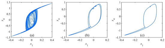
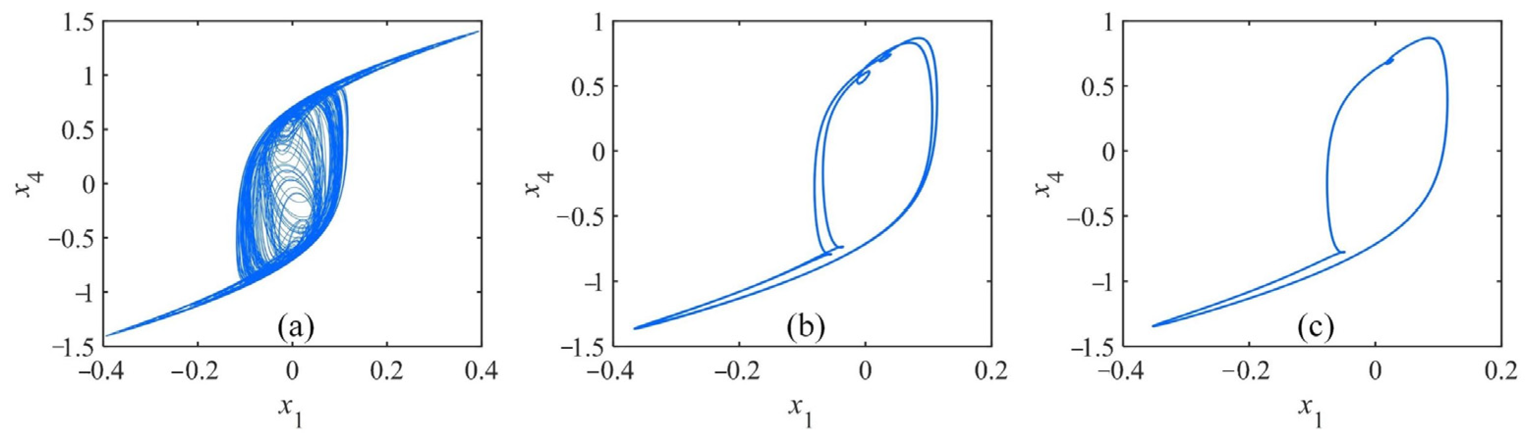
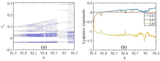
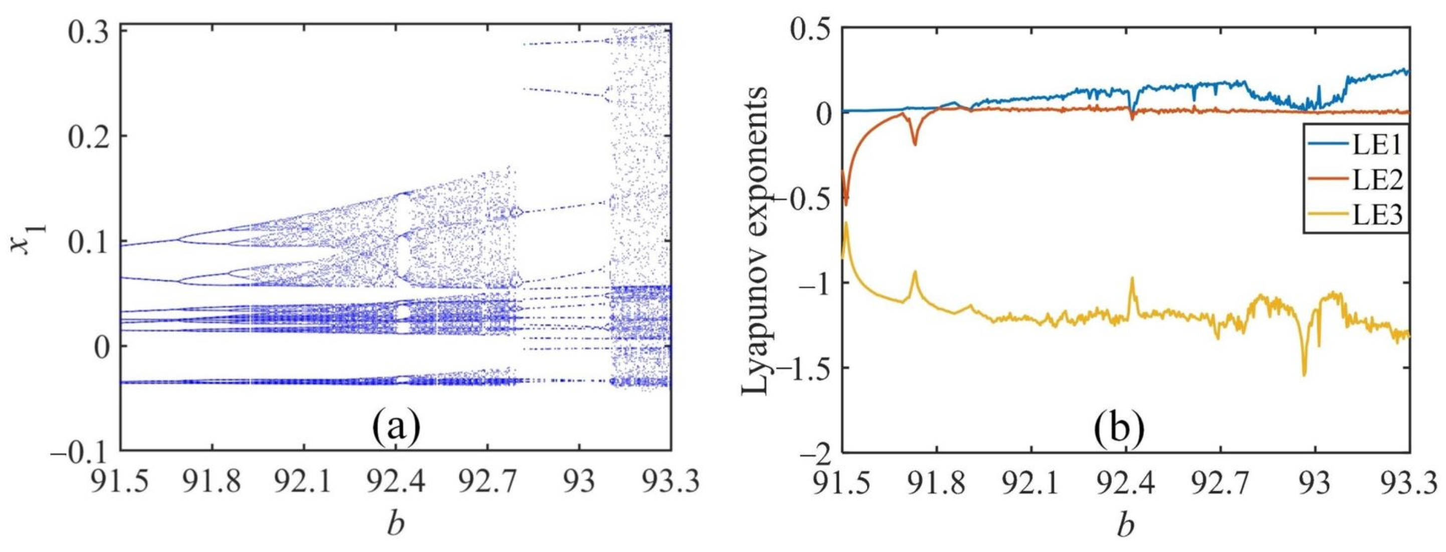
Setting the order q = 0.985, parameter a = 6, initial values x₀ = (0.1, 0.1, 0.1, 1.5, 0.1), analyzing dynamical characteristics of the system when b changes from 91.5 to 93.3, the bifurcation diagram compared with Lyapunov exponential spectrum is portrayed in Figure 12. The system maintains an asymptotic period state at the beginning when b ∈ (91.5, 91.8). As b = 91.6, asymptotic periodic behavior is shown in Figure 13. Then, the system gradually behaves as a chaotic state after period-doubling bifurcation. A narrow period window appears at b = 92.4. The other wide period window is b ∈ (92.8, 93.1). In addition, when b is given other values, the system keeps in a chaotic state. The attractor for different b values is shown in Figure 14. It can be found that the structure of the chaotic attractor is distinctive when b changes. As parameter b grows, the fractional order CNN system exhibits abundant dynamical characteristics.

Figure 12. Dynamical behavior with b ∈ [91.5, 93.3], q = 0.985, a = 6: (a) Bifurcation diagram; (b) LEs.

Figure 13. Asymptotic periodic behavior with b = 91.6: (a) Time sequences; (b) Phase diagram of the asymptotic periodic attractor.

Figure 14. Phase diagrams with q = 0.985, a = 6: (a) b = 91.6; (b) a = 92.5; (c) a = 93.3.

3.3. Coexistence of Attractors

3.3.1. Coexisting Attractors Changing with Template Parameter a

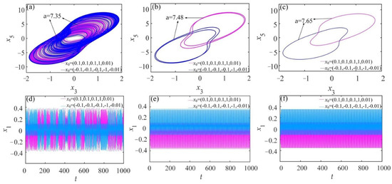
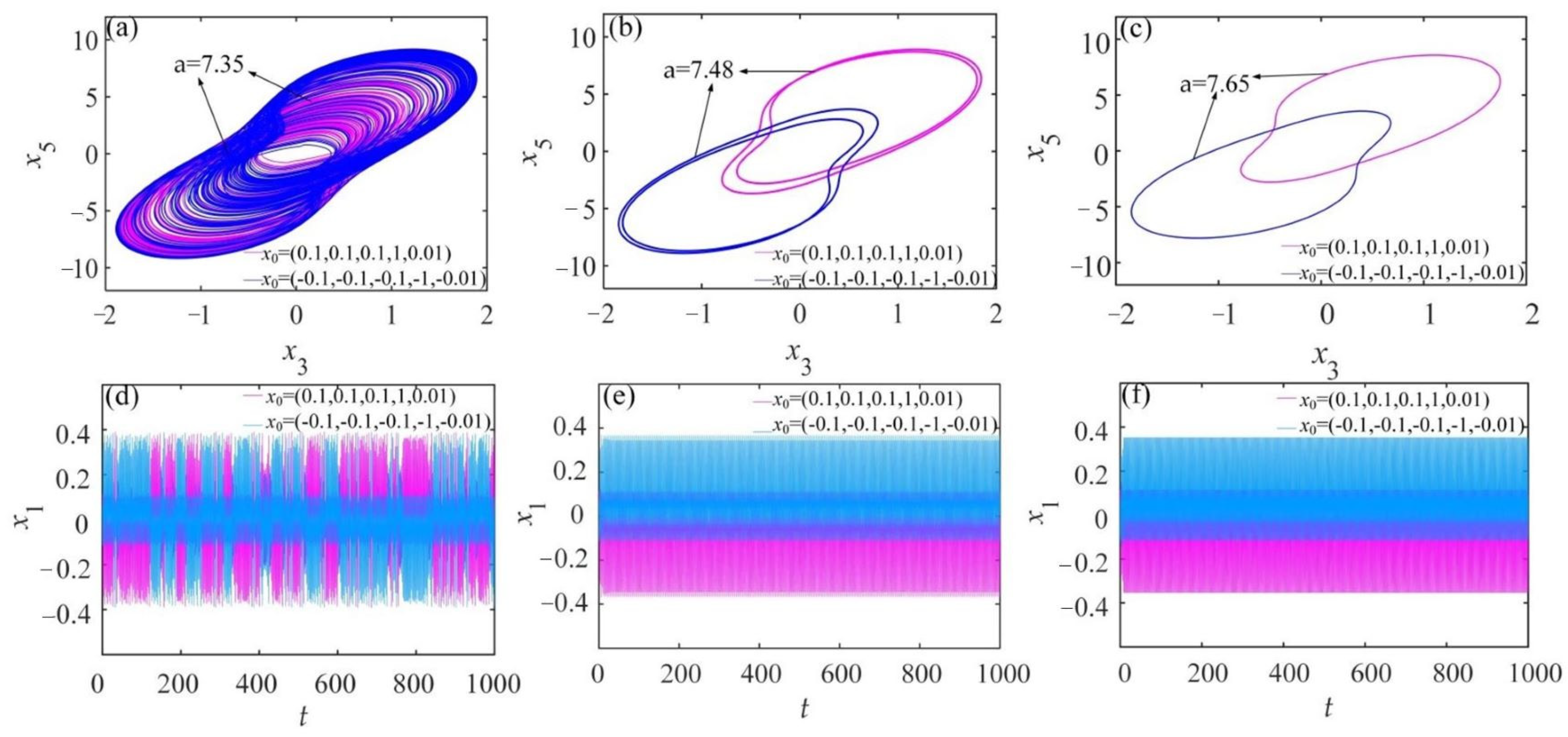
The high sensitivity to initial conditions is an essential feature of chaos. The attractor varies if the initial values are changed, and it is a significant factor in producing attractor coexistence. The coexistence of diverse attractors was discovered in the fractional order CNN system through dynamical analysis. It is worth mentioning that the coexistence under consideration here is in the long-time mode. Setting parameter q = 0.985, b = 100, selecting initial values x₀ as (0.1, 0.1, 0.1, 1, 0.01) and (−0.1, −0.1, −0.1, −1, −0.01) separately, various attractor coexistence phase diagram and time sequence diagram are displayed in Figure 15. When a = 7.35, two similar chaotic attractors blend with each other. As a increases to 7.48, the chaotic attractor degenerates into the coexistence of two pairs of limit loops. When a grows to 7.65, attractor coexistence turns into a pair of limit loops. It can be demonstrated that there is a conversion from a chaotic attractor coexistence state gradually to asymptotic periodic attractor coexistence as an increasing a within a certain range.

Figure 15. Attractor coexistence about template parameter a with q = 0.95, b = 100. Pink represents x₀ = (0.1, 0.1, 0.1, 1, 0.01) and blue represents x₀ = (−0.1, −0.1, −0.1, −1, −0.01): (a–c) x₁-x₃ phase plane; (d–f) time sequences.

3.3.2. Coexisting Attractors Changing with Template Parameter b

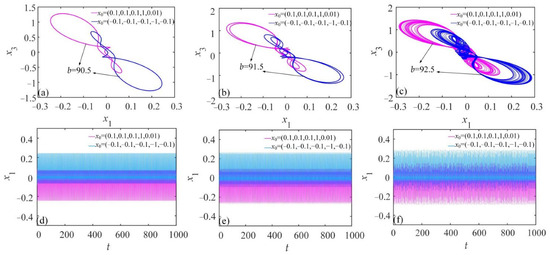
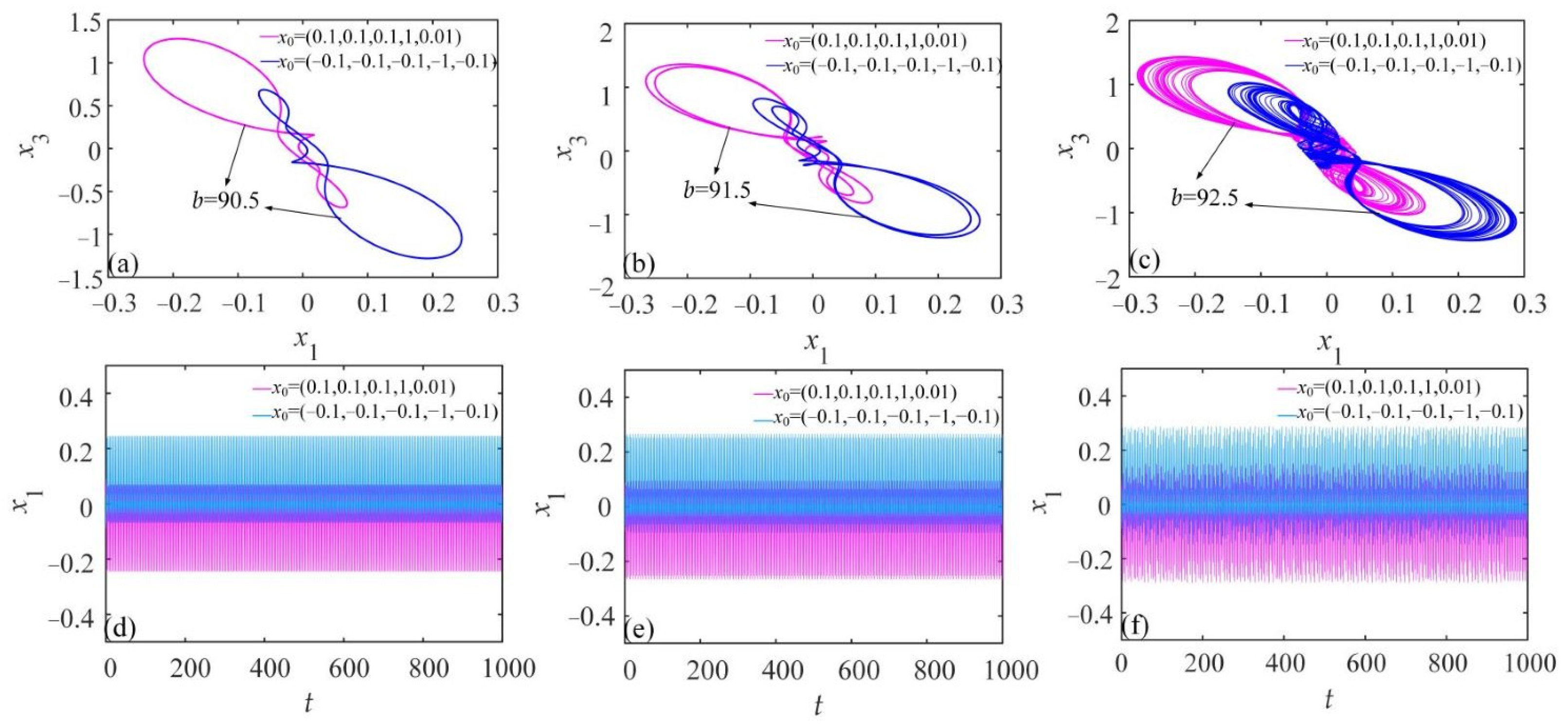
Similarly, changing parameter b, interesting shifts of attractor coexistence arise. Fixing parameter a = 6, q = 0.95, and choosing initial values x₀ as (0.1, 0.1, 0.1, 1, 0.1) and (−0.1, −0.1, −0.1, −1, −0.1), respectively, as template parameter b is altered, the attractor coexistence phase diagram and time sequence diagram are depicted in Figure 16. When b = 90.5, coexisting limit loops symmetric about the origin are partially twisted. Correspondingly, the time series are regular, and the magnitudes of limit loops are in symmetry with the time axis. As b increases to 91.5, two pairs of limit loops coexist. When b grows to 92.5, two twisted scroll chaotic attractors coupled symmetrically coexist. In the meantime, the time series corresponding to the two initial values are irregularly merged.

Figure 16. Attractor coexistence about template parameter b with q = 0.985, a = 6. Pink represents x₀ = (0.1, 0.1, 0.1, 1, 0.01) and blue represents x₀ = (−0.1, −0.1, −0.1, −1, −0.1): (a–c) x₁ − x₃ phase plane; (d–f) time sequences.

3.3.3. Coexisting Hyperchaotic Attractor with Order q

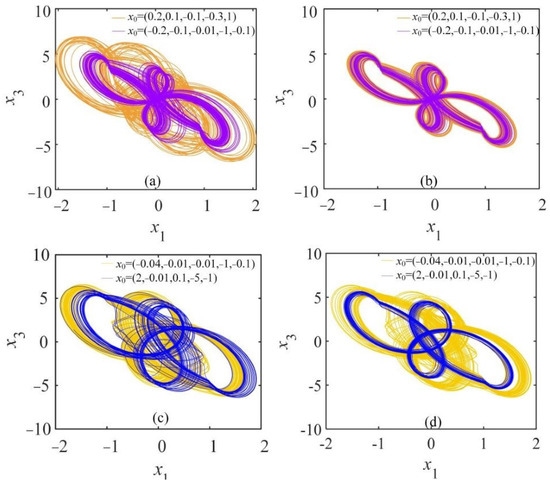
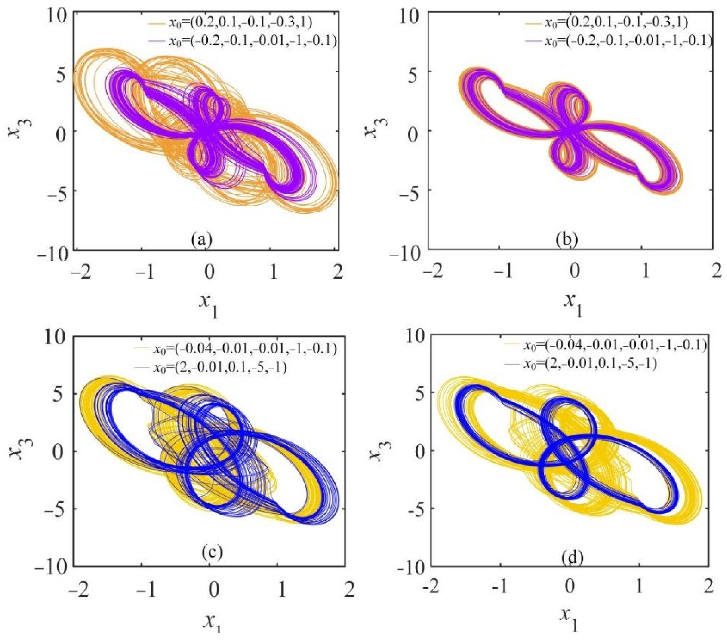
In addition to the coexistence of chaotic attractors found in the system, hyperchaotic attractor coexistence has been discovered as well. Setting parameter a = 12, b = 201, selecting initial values x0 as (0.2, 0.1, −0.1, −0.3, 1) and (−0.2, −0.1, −0.01, −1, −0.1), respectively, as the value of q changes in the hyperchaotic range, the hyperchaotic attractor coexistence occurs. When q = 0.9, two hyperchaotic attractors of different sizes coexist in Figure 17a. As q increases to 9.25, a pair of similar hyperchaotic attractors coexist in the diagram Figure 17b. Then, when q = 0.94 and q = 0.92, setting parameter a = 13, b = 200, and selecting initial values x₀ as (−0.04, −0.01, −0.01, −1, −0.1) and (2, −0.01, 0.1, −5, −1), the hyperchaotic attractor coexistence phase diagram are displayed in Figure 17c,d. Clearly, hyperchaotic attractor coexistence varies with the change of order q.

Figure 17. Hyperchaotic attractor coexistence: (a) q = 0.9, when a = 12, b = 201,orange represents x₀ = (0.2, 0.1, −0.1, −0.3, 1) and pink represents x₀ = (−0.2, −0.1, −0.01, −1, −0.1); (b) q = 0.925, when a = 12, b = 201; (c) q = 0.94, when a = 13,b = 200; (d) q = 0.92, when a = 13, b = 200, yellow represents x₀ = (−0.04, −0.01, −0.01, −1, −0.1) and blue represents x₀ = (2, −0.01, 0.1, −5, −1).

3.4. State Transition

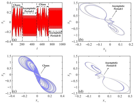
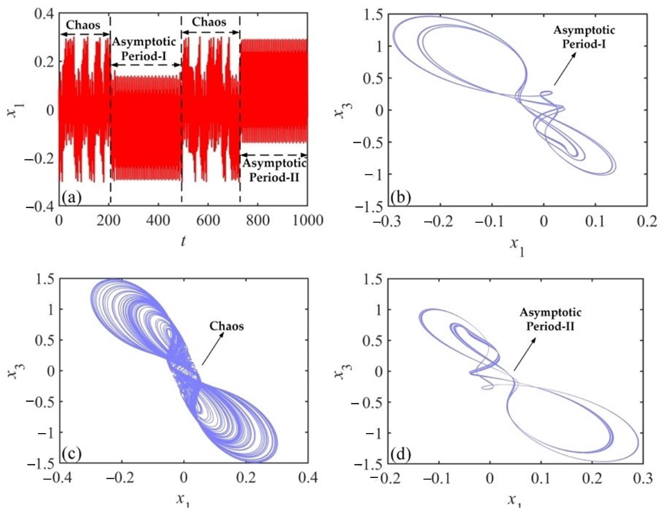
The state transition is a common phenomenon in systems that are capable of generating chaos. The state transition is associated with a shift of dynamical behaviors. Chaotic and asymptotic periodic states of fractional order systems are interchanged in this process. Transient chaos lasts for a relatively short time, and it can occur in the course of a state transition. When the parameters are modified as the order q = 0.985, a = 6, b = 93.093, and the initial value is (0.1, 0.1, 0.1, 1.5, 0.1), state transitions between different dynamical states have occurred in the system.

With a sampling time h = 0.01 and a total number of samples N = 100,000, the time sequence about variable x₁ is presented in Figure 18a. Obviously, two episodes of transient chaos have appeared in the system during these 1000 s. When 0 s < t < 200 s, the system behaves as its first temporary chaotic state. As 200 s < t < 500 s, there is an asymptotic periodic state (Asymptotic Period-I) that undergoes a transition from the chaotic condition. When 500 s < t < 725 s, the chaotic attractor reappears in the form of Figure 18c. When 725 s < t < 1000 s, the system transforms into another asymptotic periodic state (Asymptotic Period-II). The attractor phase diagrams for the two asymptotic periodic states are drawn in Figure 18b,d, observing the attractor at asymptotic period-I is apparently different from asymptotic period-II.

Figure 18. State transition in CNN system: (a) Time sequence of x₁; (b) Asymptotic period-I attractor trajectory about the x₁ − x₃ plane; (c) The chaos attractor trajectory about the x₁ − x₃ plane; (d) Asymptotic period-II attractor trajectory about the x₁ − x₃ plane.

3.5. Complexity of CNN System

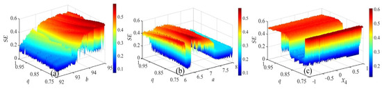
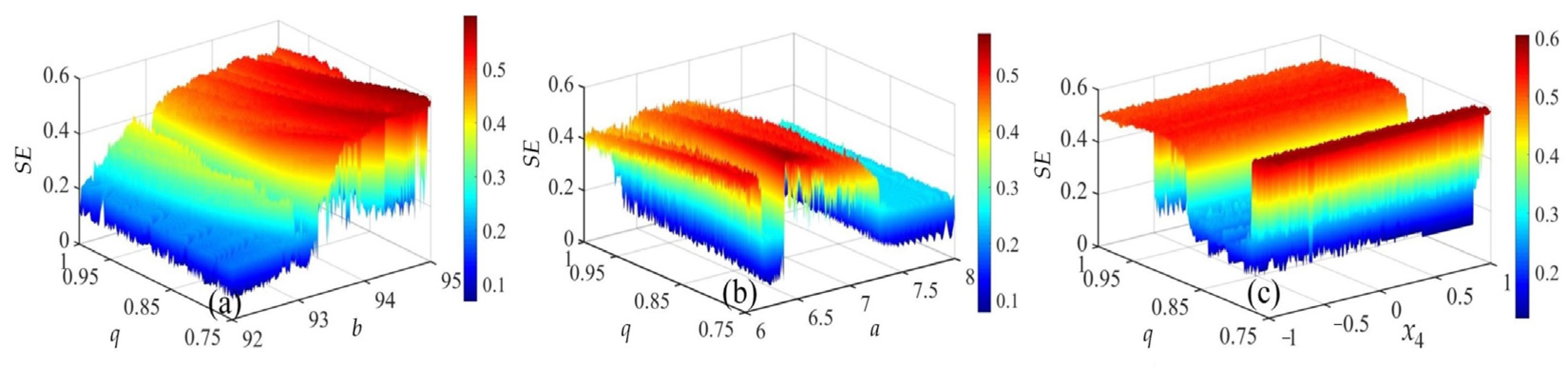
Complexity is another common way to describe the dynamical behaviors of chaotic systems. The value of complexity can be obtained by a multitude of algorithms for measuring the degree to how near chaotic sequences are to random sequences. The spectral entropy (SE) method calculates complexity values by combining the energy distribution and the Shannon entropy. The SE is a fast and real-time method of calculation. The three-dimensional SE complexity diagram is directly illustrated in Figure 19.

Figure 19. Complexity of different parameters plane: (a) 3D complexity diagram for q ∈ [0.75, 1], a ∈ [6, 8], b = 100; (b) 3D complexity diagram for q ∈ [0.75, 1], b ∈ [92, 95], a = 6; (c) 3D complexity diagram for initial value x₄ ∈ [−1, 1], a = 6, b = 95.

The parameter a, b, initial value x₄ or order q value ranges form a numerical plane region, with complexity values expressed as colored height levels. When the color of the region is closer to red, the complexity is higher, indicating that chaotic series gets closer to random number sequences. In contrast, when the color becomes more blue, the complexity is lower. Three-dimensional diagrams reflect the complexity corresponding to any point in the numerical plane in the CNN system. To a certain extent, it offers a guideline for picking the suitable system parameter and order. In practice, sequences of larger complexity are chosen for encryption applications.

4. DSP Implementation of the Fractional-Order CNN System

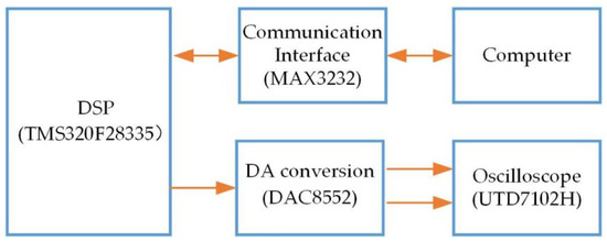
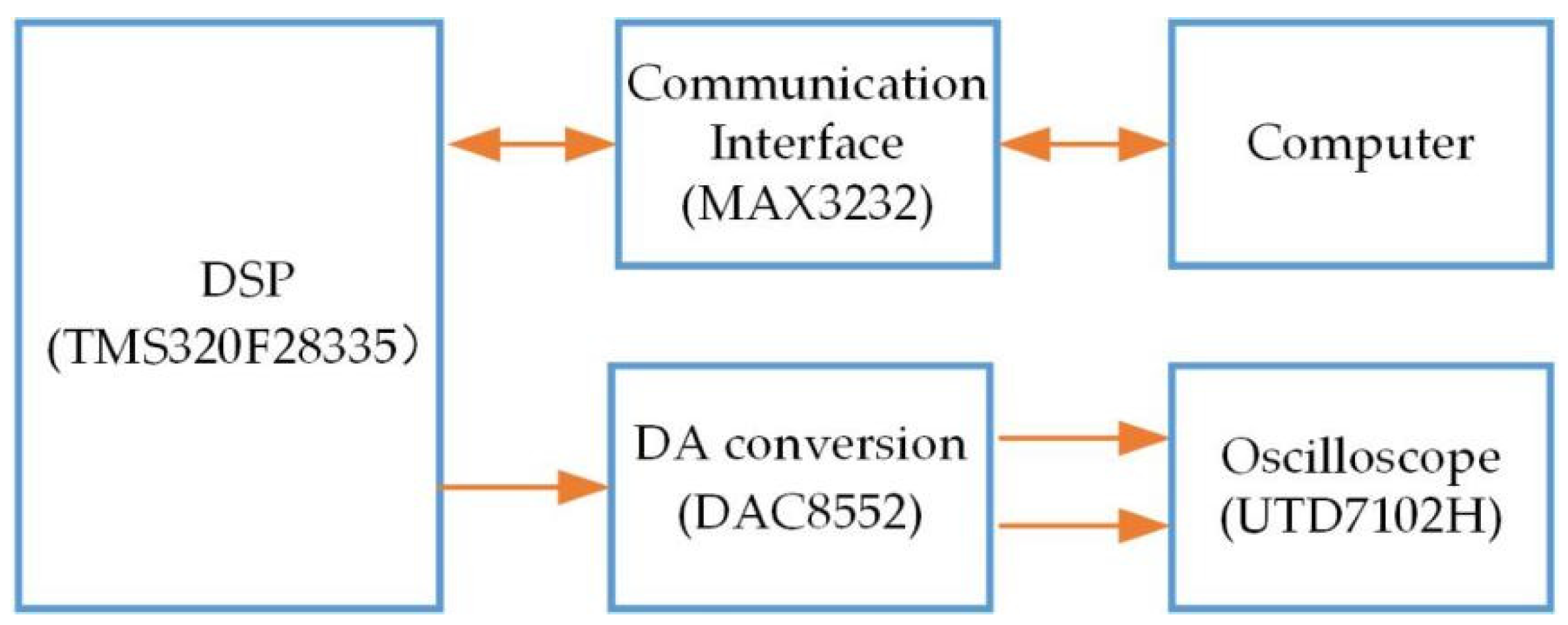
There is a growing trend to implement fractional-order chaotic systems using digital processing techniques in integrated circuits [23,49,50]. DSP implementation of chaotic systems is relatively easy and inexpensive. The DSP core chip type used is 32-bit TMS320F28335, which has an internal floating-point computing unit. Powerful digital signal processing capability makes it a great advantage in implementing fractional-order dynamical systems. The design of the system hardware structure follows the module as shown in Figure 20. Dual-channel DA converter DAC8552 converts DSP-generated chaotic sequences to analog signals. The analog signal output is displayed as an attractor phase diagram in the oscilloscope UTD7102H. The communication interface MAX3232 is responsible for connecting the DSP to the computer. The integrated development environment for DSP implementation on the computer is Code Composer Studio 6.0.0.

Figure 20. Hardware block diagram of DSP implementation.

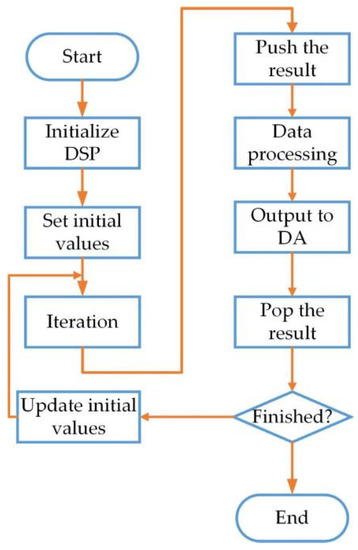
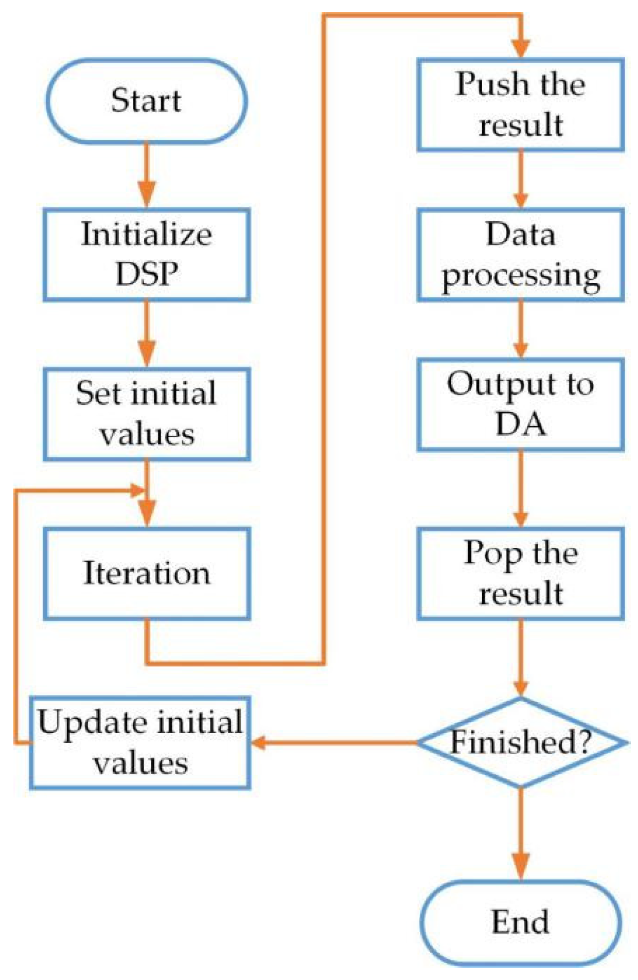
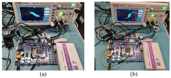
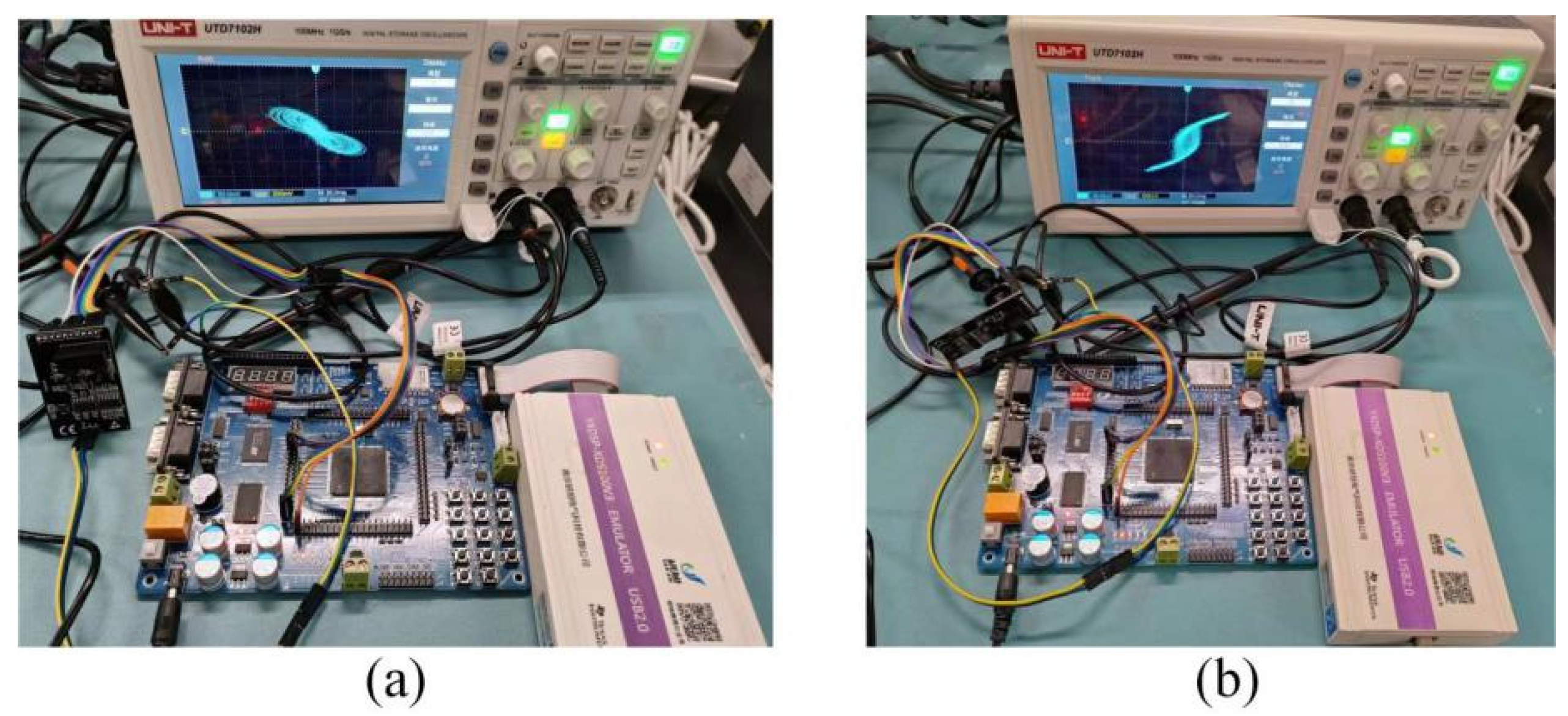
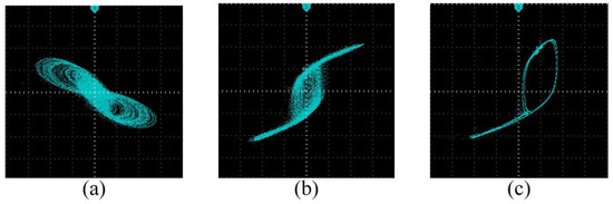
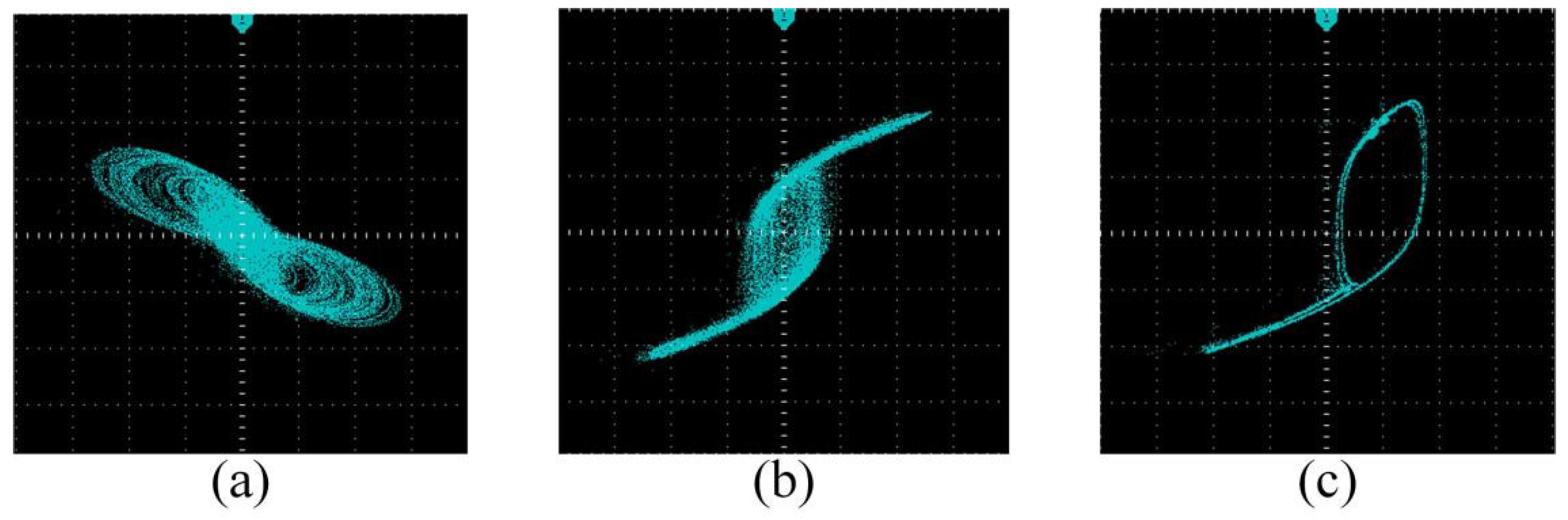
The concrete software design process is depicted in Figure 21. First of all, DSP is initialized and with parameters and initial values properly set. Subsequently, the result of each computation is pushed into the stack for iterative operation. The data go through the processing of adding positive integers and amplifying. Then, data results are transferred to the DA converter and displayed in the form of attractor phase diagrams in oscilloscope. According to Figure 20, the physical diagram of the hardware connection for this experiment is shown in Figure 22. During this experiment, the same parameters and initial conditions are set as the Figure 11. After debugging, chaotic and asymptotic periodic attractors in a long-time mode are presented in the oscilloscope as is shown in Figure 23. It is evident that the DSP realization results of the system are in accordance with simulation results.

Figure 21. DSP implementation process.

Figure 22. DSP hardware connection with q = 0.95, a=7.25, b = 100, x₀ = (0.1, 0.01, 0.1, 1, 0.1): (a) x₁ − x₃ plane; (b) x₁ − x₄ plane.

Figure 23. Attractors result based on the DSP with q = 0.95, b = 100, x₀ = (0.1, 0.01, 0.1, 1, 0.1): (a) x₁ − x₃ plane when a = 7.25; (b) x₁ − x₄ plane when a = 7.25; (c) x₁ − x₄ plane when a = 7.48.

5. Conclusions

In this paper, a new fractional-order CNN system with a hyperbolic tangent activation function is constructed and analyzed. ADM is used to solve this system accurately and efficiently. The equilibrium point is also calculated and clarified to demonstrate the stability of the system. The phase diagram, bifurcation diagram, Lyapunov Exponent spectrum (LEs), and spectral entropy (SE) complexity algorithm are used to analyze the dynamical characteristics of the fractional-order CNN system. As the order q, template parameters a,b, and initial values x₀ are varied, the study results indicate the system exhibits complex dynamical behaviors. The hyperchaotic attractor occurs in the process of changing the order. Changing the template parameters in the system, various kinds of asymptotic periodic and chaotic attractors appear. The influence of different parameters on the system state is different. Many types of coexistence phenomena have also been discovered, including symmetric attractor coexistence about the origin and hyperchaotic attractor coexistence. Surprisingly, when adjusting parameters, state transition phenomena appear as well. The three-dimensional complexity is altered when parameters are adjusted, indicating that the system can generate chaotic pseudo-random sequences with large complexity. This feature ensures high security and reliability in the application of secure communications and image encryption. The results of the SE complexity algorithm provide a theoretical basis for selecting the appropriate parameters. Digital circuit design and implementation is finished based on DSP development board, which confirms the digital feasibility of the fractional-order CNN system. In the following work, the system can be applied to the encryption field such as image, audio and video.

References

- Lin, H.; Wang, C.; Chen, C.; Sun, Y.; Zhou, C.; Xu, C.; Hong, Q. Neural bursting and synchronization emulated by neural networks and circuits. IEEE Trans. Circuits Syst. I Regul. Pap. 2021, 68, 3397–3410. [Google Scholar] [CrossRef] [Scilit]
- Chen, M.; Qi, J.; Xu, Q.; Bao, B. Quasi-period, periodic bursting and bifurcations in memristor-based FitzHugh-Nagumo circuit. AEUE-Int. J. Electron. Commun. 2019, 110, 152840. [Google Scholar] [CrossRef] [Scilit]
- Ma, T.; Mou, J.; Yan, H.; Cao, Y. A new class of hopfield neural network with double memristive synapses and its DSP implementation. Eur. Phys. J. Plus 2022, 137, 1135. [Google Scholar] [CrossRef] [Scilit]
- Ma, J.; Tang, J. A review for dynamics in neuron and neuronal network. Nonlinear Dyn. 2017, 89, 1569–1578. [Google Scholar] [CrossRef] [Scilit]
- Yang, F.; Wang, X. Dynamic characteristic of a new fractional-order chaotic system based on the hopfield neural network and its digital circuit implementation. Phys. Scr. 2021, 96, 035218. [Google Scholar] [CrossRef] [Scilit]
- Chua, L.O.; Yang, L. Cellular neural networks: Theory. IEEE Trans. Circuits Syst. 1988, 35, 1257–1271. [Google Scholar] [CrossRef] [Scilit]
- Di Marco, M.; Forti, M.; Tesi, A. Complex dynamics in nearly symmetric three-cell cellular neural networks. Int. J. Bifurc. Chaos 2002, 12, 1267–1293. [Google Scholar] [CrossRef] [Scilit]
- Makoto, I. RTD-based cellular neural networks with multiple steady states. Int. J. Bifurc. Chaos 2001, 11, 2913–2959. [Google Scholar]
- Chen, F.; Li, J.; Chen, F. Chaos for discrete-time RTD-based cellular neural networks. Int. J. Bifurc. Chaos 2007, 17, 4395–4401. [Google Scholar] [CrossRef] [Scilit]
- Zou, F.; Nossek, J.A. Bifurcation and chaos in cellular neural networks. IEEE Trans. Circuits Syst. I Regul. Pap. 1993, 40, 166–173. [Google Scholar] [CrossRef] [Scilit]
- Wang, L.; Liu, W.; Shi, H.; Zurada, J.M. Cellular neural networks with transient chaos. IEEE Trans. Circuits Syst. II Express Briefs 2007, 54, 440–444. [Google Scholar] [CrossRef] [Scilit]
- Chen, F.; Li, J. Hypechaos in RTD-based cellular neural networks. Int. J. Bifurc. Chaos 2008, 18, 3439–3446. [Google Scholar] [CrossRef] [Scilit]
- Xiu, C.; Zhou, R.; Liu, Y. New chaotic memristive cellular neural network and its application in secure communication system. Chaos Solitons Fractals Interdiscip. J. Nonlinear Sci. Nonequilibrium Complex Phenom. 2020, 141, 110316. [Google Scholar] [CrossRef] [Scilit]
- Gao, X.; Mou, J.; Banerjee, S.; Zhang, Y. Color-gray multi-image hybrid compression-encryption scheme based on BP neural network and knight tour. IEEE Trans. Cybern. 2023, 53, 5037–5047. [Google Scholar] [CrossRef] [Scilit] [PubMed]
- Sha, Y.; Mou, J.; Wang, J.; Banerjee, S.; Sun, B. Chaotic image encryption with Hopfield neural network. Fractals 2023, 31, 2340107. [Google Scholar] [CrossRef] [Scilit]
- Chua, L.O.; Yang, L. Cellular neural networks: Applications. IEEE Trans. Circuits Syst. 1988, 35, 1273–1290. [Google Scholar] [CrossRef] [Scilit]
- Kumar, A.; Das, S.; Yadav, V.K.; Rajeev; Cao, J.; Huang, C. Synchronizations of fuzzy cellular neural networks with proportional time-delay. Aims Math. 2021, 6, 10620–10642. [Google Scholar] [CrossRef] [Scilit]
- Norouzi, B.; Mirzakuchaki, S. An image encryption algorithm based on DNA sequence operations and cellular neural network. Multimed. Tools Appl. 2017, 76, 13681–13701. [Google Scholar] [CrossRef] [Scilit]
- Zhang, R.; Yu, L.; Jiang, D.; Ding, W.; Song, J.; He, K.; Ding, Q. A novel plaintext-related color image encryption scheme based on cellular neural network and Chen’s chaotic system. Symmetry 2021, 13, 393. [Google Scholar] [CrossRef] [Scilit]
- Wang, X.; Su, Y.; Luo, C.; Wang, C. A novel image encryption algorithm based on fractional order 5D cellular neural network and Fisher-Yates scrambling. PLoS ONE 2020, 15, e0236015. [Google Scholar] [CrossRef] [Scilit]
- Du, F.; Lu, J. Finite-time synchronization of fractional-order delayed fuzzy cellar neural networks with parameter uncertainties. IEEE Trans. Fuzzy Syst. 2022, 31, 1769–1779. [Google Scholar] [CrossRef] [Scilit]
- Han, X.; Mou, J.; Xiong, L.; Ma, C.; Liu, T.; Cao, Y. Coexistence of infinite attractors in a fractional-order chaotic system with two nonlinear functions and its DSP implementation. Integration 2021, 81, 43–55. [Google Scholar] [CrossRef] [Scilit]
- Qin, C.; Sun, K.; He, S. Characteristic analysis of fractional-order memristor-based hypogenetic jerk system and its DSP implementation. Electronics 2021, 10, 841. [Google Scholar] [CrossRef] [Scilit]
- Ren, L.; Li, S.; Banerjee, S.; Mou, J. A new fractional-order complex chaotic system with extreme multistability and its implementation. Phys. Scr. 2023, 98, 055201. [Google Scholar] [CrossRef] [Scilit]
- Liu, X.; Mou, J.; Wang, J.; Banerjee, S.; Li, P. Dynamical analysis of a novel fractional-order chaotic system based on memcapacitor and meminductor. Fractal Fract. 2022, 6, 671. [Google Scholar] [CrossRef] [Scilit]
- Can, N.H.; Nikan, O.; Rasoulizadeh, M.N.; Jafari, H.; Gasimov, Y.S. Numerical computation of the time non-linear fractional generalized equal width model arising in shallow water channel. Therm. Sci. 2020, 24 (Suppl. 1), 49–58. [Google Scholar] [CrossRef]
- Salama, F.M.; Ali, N.H.M.; Hamid, N.N.A. Fast O (N) hybrid Laplace transform-finite difference method in solving 2D time fractional diffusion equation. J. Math. Comput. Sci. 2021, 23, 110–123. [Google Scholar] [CrossRef] [Scilit]
- Jassim, H.K.; Shareef, M.A. On approximate solutions for fractional system of differential equations with Caputo-Fabrizio fractional operator. J. Math. Comput. Sci. 2021, 23, 58–66. [Google Scholar] [CrossRef] [Scilit]
- Akram, T.; Abbas, M.; Ali, A. A numerical study on time fractional Fisher equation using an extended cubic B-spline approximation. J. Math. Comput. Sci. 2021, 22, 85–96. [Google Scholar] [CrossRef] [Scilit]
- Kang, Y.-M.; Xie, Y.; Lu, J.-C.; Jiang, J. On the nonexistence of non-constant exact periodic solutions in a class of the Caputo fractional-order dynamical systems. Nonlinear Dyn. 2015, 82, 1259–1267. [Google Scholar] [CrossRef] [Scilit]
- Sun, H.; Abdelwahab, A.; Onaral, B. Linear approximation of transfer function with a pole of fractional power. IEEE Trans. Autom. Control 1984, 29, 441–444. [Google Scholar] [CrossRef] [Scilit]
- Diethelm, K.; Ford, N.J.; Freed, A.D. A predictor-corrector approach for the numerical solution of fractional differential equations. Nonlinear Dyn. 2002, 29, 3–22. [Google Scholar] [CrossRef] [Scilit]
- Adomian, G. A new approach to nonlinear partial differential equations. J. Math. Anal. Appl. 1984, 102, 420–434. [Google Scholar] [CrossRef] [Scilit]
- Tavazoei, M.S.; Haeri, M. Unreliability of frequency-domain approximation in recognising chaos in fractional-order systems. IET Signal Process. 2007, 1, 171–181. [Google Scholar] [CrossRef] [Scilit]
- Ma, C.; Mou, J.; Yang, F.; Yan, H. A fractional-order hopfield neural network chaotic system and its circuit realization. Eur. Phys. J. Plus 2020, 135, 100. [Google Scholar] [CrossRef] [Scilit]
- Ma, T.; Mou, J.; Li, B.; Banerjee, S.; Yan, H. Study on the complex dynamical behavior of the fractional-order hopfield neural network system and its implementation. Fractal Fract. 2022, 6, 637. [Google Scholar] [CrossRef] [Scilit]
- Zheng, Y.; Ji, Z. Predictive control of fractional-order chaotic systems. Chaos Solitons Fractals 2016, 87, 307–313. [Google Scholar] [CrossRef] [Scilit]
- Jahanshahi, H.; Zambrano-Serrano, E.; Bekiros, S.; Wei, Z.; Volos, C.; Castillo, O.; Aly, A.A. On the dynamical investigation and synchronization of variable-order fractional neural networks: The Hopfield-like neural network model. Eur. Phys. J. Spec. Top. 2022, 231, 1757–1769. [Google Scholar] [CrossRef] [Scilit]
- Huang, X.; Zhao, Z.; Wang, Z.; Li, Y. Chaos and hyperchaos in fractional-order cellular neural networks. Neurocomputing 2012, 94, 13–21. [Google Scholar] [CrossRef] [Scilit]
- Ilsang, O.; Yongdai, K. Smooth function approximation by deep neural networks with general activation functions. Entropy 2019, 21, 627. [Google Scholar]
- Han, Q.; Liao, X.; Huang, T.; Peng, J.; Li, C.; Huang, H. Analysis and design of associative memories based on stability of cellular neural networks. Neurocomputing 2012, 97, 192–200. [Google Scholar] [CrossRef] [Scilit]
- Nakagawa, M. On the chaos neuron models with chebyshev type activation functions. J. Phys. Soc. Jpn. 2020, 90, 014001. [Google Scholar] [CrossRef] [Scilit]
- Liu, Y.; Song, Z.; Tan, M. Multiple µ-stability and multiperiodicity of delayed memristor-based fuzzy cellular neural networks with nonmonotonic activation functions. Math. Comput. Simul. 2019, 159, 1–17. [Google Scholar] [CrossRef] [Scilit]
- Amanda, C.M.; Paulo, C.R. Hopfield neural network: The hyperbolic tangent and the piecewise-linear activation functions. Neural Netw. 2012, 34, 42–45. [Google Scholar] [CrossRef] [Scilit]
- Ma, T.; Mou, J.; Al-Barakati, A.A.; Jahanshahi, H.; Li, S. Coexistence behavior of a double-MR-based cellular neural network system and its circuit implementation. Nonlinear Dyn. 2023, 111, 11593–11611. [Google Scholar] [CrossRef] [Scilit]
- Rajput, G.; Raut, G.; Chandra, M.; Vishvakarma, S.K. VLSI implementation of transcendental function hyperbolic tangent for deep neural network accelerators. Microprocess. Microsyst. 2021, 84, 104270. [Google Scholar] [CrossRef] [Scilit]
- Shakiba, F.M.; Zhou, M. Novel analog implementation of a hyperbolic tangent neuron in artificial neural networks. IEEE Trans. Ind. Electron. 2020, 68, 10856–10867. [Google Scholar] [CrossRef] [Scilit]
- Arena, P.; Baglio, S.; Fortuna, L.; Manganaro, G. Chua’s circuit can be generated by CNN cells. IEEE Trans. Circuits Syst. I Fundam. Theory Appl. 1995, 42, 123–125. [Google Scholar] [CrossRef] [Scilit]
- Malik, S.A.; Mir, A.H. FPGA realization of fractional order neuron. Appl. Math. Model. 2020, 81, 372–385. [Google Scholar] [CrossRef] [Scilit]
- Sharma, A.; Rawat, T.K. Design and FPGA implementation of lattice wave fractional order digital differentiator. Microelectron. J. 2019, 88, 67–78. [Google Scholar] [CrossRef] [Scilit]
Disclaimer/Publisher’s Note: The statements, opinions and data contained in all publications are solely those of the individual author(s) and contributor(s) and not of MDPI and/or the editor(s). MDPI and/or the editor(s) disclaim responsibility for any injury to people or property resulting from any ideas, methods, instructions or products referred to in the content. |
© 2023 by the authors. Licensee MDPI, Basel, Switzerland. This article is an open access article distributed under the terms and conditions of the Creative Commons Attribution (CC BY) license (https://creativecommons.org/licenses/by/4.0/).