Article

Image Enhancement Model Based on Fractional Time-Delay and Diffusion Tensor

1
School of Mathematics, Harbin Institute of Technology, Harbin 150001, China
2
School of Physics, Harbin Institute of Technology, Harbin 150001, China
*
Author to whom correspondence should be addressed.
Fractal Fract. 2023, 7(8), 569; https://doi.org/10.3390/fractalfract7080569
Submission received: 9 June 2023 / Revised: 20 July 2023 / Accepted: 21 July 2023 / Published: 25 July 2023
(This article belongs to the Special Issue Advances in Fractional Order Derivatives and Their Applications)

Abstract

:
Image enhancement is one of the bases of image processing technology, which can enhance useful features and suppress useless information of images according to the specified task. In order to ensure coherent enhancement for images with oriented flow-like structures, we propose a nonlinear diffusion system model based on time-fractional delay. By combining the nonlinear isotropic diffusion equation with fractional time-delay regularization, we construct a structure tensor. Meanwhile, the introduction of source terms enhances the contrast of the image, making it effective for denoising images with high-level noise. Based on compactness principles, the existence of weak solutions for the model is proved by using the Galerkin method. In addition, various experimental results verify the enhancement ability of the proposed model.

1. Introduction

Image processing technology is widely used in fields such as medical image processing, text recognition and speech recognition, and unmanned driving. As an important part of image processing technology, image enhancement focuses on enhancing the useful information in the image and improving the clarity of the image. In recent years, many enhancement methods for digital images have been proposed, roughly divided into four categories: spatial domain-based methods [1,2], frequency domain-based methods [3,4], deep learning-based methods [5,6], and partial differential equations-based method. The spatial domain-based method has fast computation speed but cannot provide relevant information between pixels. The frequency domain-based method can provide detailed information but it requires a large amount of computation. The image enhancement algorithm based on deep learning can learn the complex transformation of an image, but its training time is long and it lacks interpretability. The method based on partial differential equations has always played a significant role in the field of image processing, which was firstly elaborated by Gabor [7] and Jain [8]. This method is based on strong mathematical theories. Its basic idea is to evolve the initial image through partial differential equations and obtain the enhanced image.
In this paper, we focus on the problem of image enhancement with oriented flow-like structures. These structures usually exist in the fields of fluid mechanics, geology and biology, texture analysis, computer vision and image processing. In the development of image processing using partial differential equations, the most classic model is the PM model proposed by Perona and Malik et al. [9]. Based on the PM model, the integer-order isotropic diffusion equation was developed rapidly, such as the viscoelastic equation and wave equation, which further stimulated the emergence of the anisotropic diffusion equation. Nitzberg [10] and Cottet et al. [11] pioneered the description and analysis of various anisotropic diffusion methods. Furthermore, Weickert’s work about diffusion tensors greatly promoted the research on anisotropic diffusion methods in the field of image processing. They proposed a multi-scale method that successfully completes the connection of interruption lines and the enhancement of flow-like structures. In this model, operators of interest, such as second-order moment matrices and structural tensors, are used to control nonlinear diffusion filtering. Since then, many scholars have conducted extensive research about this method [12,13,14,15,16,17,18]. For examples, Nnolim et al. [17] described a fuzzy image contrast enhancement algorithm based on a modified partial differential equation. The algorithm utilizes multi-scale local global enhancement of logarithmic reflectance and illumination components. The model successfully avoids the numerous steps required by standard DCP based methods and produces good visual effects. Gu et al. [18] proposed a SAR image enhancement method combining the PM nonlinear equation and coherent enhancement partial differential equation. The mixture model not only avoids noise enhancement but also enhances image edges.
Along with the development of image processing for integer-order partial differential equations, fractional-order partial differential equations [19,20,21,22] have also been developed rapidly. For example, Bai et al. [19] proposed a new nonlinear fractional-order anisotropic diffusion equation using spatial fractional derivatives to obtain more natural images. Sharma et al. [20] proposed an image enhancement model based on fractional-order partial differential equations, which can reduce the impact of noise and enhance the contrast of images nonlinearly. Chandra et al. [21] proposed a new image enhancement method based on linear fractional-order meshless partial differential equations to improve the quality of tumor images. The model can maintain fine details of smooth regions while denoising, and can nonlinearly increase the high-frequency information of the image. Ben-loghfyry [23], based on anisotropic diffusion and the time-fractional derivative in the Caputo sense, proposed a new reaction–diffusion equation to restore texture images.
In order to obtain the proposed model in this paper, the four classic models involved are explained below. Weickert studied anisotropic diffusion filters and derived a coherence-enhancing diffusion (CED) equation [24]:
u t = div ( D u ) , ( x , t ) Ω × ( 0 , T ] u ( x , 0 ) = u 0 ( x ) , x Ω u n = 0 , ( x , t ) Ω × ( 0 , T ]
where n is the unit outer normal vector, u 0 is the observed image as the initial data for the diffusion equation, D : = g 1 ( J ) is a diffusion tensor, g 1 is a nonlinear diffusion filter, J is a linear structure tensor obtained by the convolution of u σ u σ and Gaussian kernel G ρ , specifically, J = G ρ ( u σ u σ ) . The nonlinear diffusion filter of the CED model is controlled by a diffusion tensor, which can interrupt lines and enhance oriented flow-like structures. Wang et al. proposed coupled diffusion equations (CDEs) instead of the traditional linear method in image restoration [14]:
u t = div ( g 1 ( J ) u ) , ( x , t ) Ω × ( 0 , T ] J i , j t = div ( g 2 ( | u σ | ) J i , j ) , ( x , t ) Ω × ( 0 , T ] u n = 0 , J 1 , 1 n = J 2 , 2 n = 0 , ( x , t ) Ω × ( 0 , T ] u ( x , 0 ) = u 0 ( x ) , J i , j ( x , 0 ) = ( u 0 u 0 ) i , j , i , j = 1 , 2 , x Ω
where g 2 ( s ) = 1 1 + ( s / K ) 2 . The CEDs combine image restoration with singularity detection and can gradually eliminate the sensitivity of parameters to the image. Diffusion-based image enhancement methods generally use a spatial regularization, while they cannot use enough historical information. To this end, Chen et al. introduced time-delay regularization and then proposed the following model [25]:
u t = div ( L ( v ) u ) λ ( u u 0 ) , ( x , t ) ( 0 , T ] τ v t + v = u σ , ( x , t ) Ω × ( 0 , T ] u ( x , 0 ) = u 0 , v ( x , 0 ) = 0 , x Ω u n = 0 , ( x , t ) Ω × [ 0 , T ]
where τ > 0 , σ 0 . u 0 is the initial image, L = λ 1 L 1 + λ 2 L 2 , L 1 = v v , L 2 = ( v ) ( v ) , λ 1 = 1 1 + k | v | 2 , λ 2 = α | v | 2 1 + k | v | 2 , k > 0 , α > 0 , v = u ˜ , u ˜ is the time-delay regularization of u. For images with high levels of noise, they perform the pre-smoothing by combining spatial regularization at a small scale with time-delay regularization, which is particularly important for preserving textures and edge structures. This method has successfully been applied to Cotte and Ayyadi models [26].
The traditional integer-order partial differential equations cannot describe complex phenomena. To this end, countless scholars have studies on fractional calculus [19,20,21,22,27,28,29,30,31,32,33], which is an extension of integer calculus and has advantages in modeling complex phenomena with memory and genetics. The image enhancement model based on fractional calculus has long-term memory and non-locality, which can fully utilize the past information of the image and describe more complex diffusion progress. For example, Ben-loghfyry et al. proposed a reaction–diffusion equation based on anisotropic diffusion and Caputo’s time-fractional derivative to restore texture images [23]:
α u t = div ( D u ) 2 λ ω , ( x , t ) Ω × ( 0 , T ) β u t = Δ ω ( f ( x ) u ) , ( x , t ) Ω × ( 0 , T ) D u , n = ω n ( x , t ) = 0 , ( x , t ) Ω × ( 0 , T ) u ( x , 0 ) = f ( x ) , ω ( x , 0 ) = ω 0 ( x ) , x Ω
where ( α , β ) ( 0 , 1 ) 2 , Ω R 2 is a bounded area, the boundary Ω is Lipschitz continuous, n is the unit outer normal vector, λ > 0 , f L 2 ( Ω ) , and D : = D ( J ρ ( u σ ) ) is a diffusion matrix based on J ρ . The memory potential of the two coupled time-fractional diffusion equations effectively guarantees the superiority of the model.
In this paper, we propose an image enhancement model coupling a nonlinear anisotropic diffusion equation, a nonlinear isotropic diffusion equation and a fractional time-delay equation. Specifically, the spatial direction of the structure tensor is regularized by nonlinear isotropic diffusion, and the temporal direction of the the structure tensor is regularized by a fractional time-delay equation. Then, the diffusion tensor of the CED is constructed by using the obtained structure tensor. Additionally, we also introduce a source term which changes the diffusion process. The proposed model can better enhance the coherence structure and contrast of images, especially in processing noisy images or low-contrast areas. It should be noted that due to the introduction of source terms, the proposed model is more suitable for handling white noise than other existing models. We prove the existence and uniqueness of weak solutions. The proposed system of image enhancement equations based on fractional time-delay and the diffusion tensor has the following characteristics:
  • The nonlinear isotropic diffusion equation is applied to make use of the spatial information in the image. The fractional time-delay equation is applied to make use of the past information of the image. The diffusion tensor of CED is applied to complete interrupted lines and enhance flow-like structures.
  • The introduced source term is used to make a contrast enhancement between the image and its background by changing the diffusion type and behavior. In addition, this term can also reduce the noise in the image.
  • Based on the theory of partial differential equations and some properties of fractional calculus, we prove the existence and uniqueness of weak solutions.
  • The comparative experimental results verify the superiority of the proposed method. It shows that this model can complete the connection of interrupted lines, enhance the contrast of images, and deepen the fluidity characteristics of various types of lines.
The paper is organized as follows. In Section 2 , we establish an image enhancement model with fractional time-delay regularization and diffusion tensors, and provide a detailed explanation of the model. Section 2.3  deduces the theoretical part of the model, defines the Galerkin estimation of the model and the form of weak solutions, and proves the existence and uniqueness of weak solutions. Section 3 mainly designs a stable and efficient numerical format for the proposed model and conducts numerical experiments on different images. Section 4  summarizes the results.

2. The Proposed Model and Its Theoretical Analysis

2.1. Preliminary Knowledge

Definition 1
([34,35]). Assume that γ is a positive rational number, γ R + , n 1 < γ n , and n 1 is a positive integer. u ( t ) is an integrable function on the interval ( 0 , T ) , then the Caputo-type fractional derivative of u with order γ is
D c γ u ( t ) = 1 Γ ( n γ ) 0 t u ( n ) ( s ) ( t s ) γ n + 1 d s , t > 0
where Γ ( · ) is a gamma function. When γ = n , the Caputo-type fractional order of order γ is a common integer-order derivative of order n, D c γ u ( t ) = u ( n ) ( t ) .
Generally, the sign of a Caputo-type fractional derivative contains information about the boundary point of the integral interval, but only the interval ( 0 , T ) is involved in this paper, so the sign is simplified to D c γ u ( t ) , which represents the right limit of u at t = 0 , which is the derivative of u ( 0 + ) when it exists.
Theorem 1
([36]). Assume that γ ( 0 , 1 ) , H is a Hilbert space and ω : [ 0 , T ] H such that ω ( t ) H 2 is absolutely continuous. Then
D c γ ω ( t ) H 2 2 ω ( t ) , D c γ ω ( t ) H
for each a.e. t ( 0 , T ] .
Proposition 1
([37]). Suppose that u ( t ) and g ( t ) are integrable functions defined on the interval ( 0 , T ) , then
0 T g ( t ) D c γ u ( t ) d t = 0 T u ( t ) D ( t , T ) γ g ( t ) d t + j = 0 n 1 D ( t , T ) γ + j n g ( t ) D n 1 j u ( t ) | 0 T
where D ( t , T ) γ g ( t ) = 1 Γ ( n γ ) ( d d t ) n t T ( t s ) n γ 1 g ( s ) d s is a Riemann–Liouville fractional derivative.

2.2. The Proposed Model

In this subsection, we propose a new image enhancement model based on fractional time-delay regularization and diffusion tensor. Assuming that Ω R n is a bounded region, Ω is a Lipschitz continuous boundary, and the mapping u : Ω R represents a positive real-valued function of the gray image u ( x ) , then we establish the following image enhancement model:
u t = div ( g 1 ( J ) u ) + λ ( u u ˜ ) , ( x , t ) Ω × ( 0 , T ] τ D c γ J i , j + J i , j = v i , j , ( x , t ) Ω × ( 0 , T ] v i , j t = div ( g 2 ( u σ ) v i , j ) , ( x , t ) Ω × ( 0 , T ] g 1 ( J ) u , n = 0 , v 1 , 1 n = v 2 , 2 n = 0 , v 1 , 2 n = v 2 , 1 n = 0 , ( x , t ) Ω × ( 0 , T ] u ( x , 0 ) = u 0 ( x ) , J i , j ( x , 0 ) = 0 , v i , j ( x , 0 ) = ( u 0 u 0 ) i , j , i , j = 1 , 2 , x Ω
where λ > 0 is an adaptive adjustment parameter, u ˜ is the average value of the image, τ > 0 is the time-delay regularization parameter, γ ( 0 , 1 ) is the fractional parameter, u σ = G σ u 0 is the image with Gaussian convolution, J = ( J i , j ) i , j = 1 , 2 is the structural tensor, n is the unit outer normal vector of Ω , g 1 is the diffusion matrix, and g 2 is the diffusion function. D c γ is the Caputo time-fractional derivative, see Definition 1. In the model, the nonlinear isotropic diffusion equation is used to spatially regularize the structure tensor, the fractional time-delay equation is used to temporally regularize the structure tensor, and the coherent enhanced diffusion tensor based on the structure tensor is used to perform anisotropic diffusion.
The interpretation of the terms of our model is as follows:
  • The first equation is an anisotropic diffusion equation, which can enhance flow-like structures and connect interrupted lines. Since the eigenvalues μ i ( i = 1 , 2 ) in J imply the coherent structure, we select κ = μ 1 μ 2 2 as the measure of coherence. More related details can be found in reference [24]. Specifically, the eigenvectors of structural tensors provide optimal choices for local directions, while the corresponding eigenvalues represent local contrast along these directions. By constructing diffusion tensor D with the same eigenvector as J and selecting appropriate eigenvalues for smoothing, it can be ensured that the model can complete the connection of interrupted lines and enhance similar flow structures. The source term in the first equation is used to change the diffusion type and behavior so as to make a contrast enhancement between the target image and the background and enhance the texture structure; more details are referred to in [38].
  • The second equation performs as a fractional time-delay regularization, which considers the past information of the image. Meanwhile, the long-range dependency of this equation can avoid excessive smoothing.
  • The final equation is based on a structure tensor; this equation is an isotropic diffusion equation, which performs well when dealing with the discontinuity. Let s = | u σ | , and choose the diffusion function g 2 ( s ) = 1 1 + ( s / K ) 2 , where K is a threshold value. Alternatively, we can choose the diffusion function as g 2 ( s ) = 1 ε + ( s ) 2 , where ε is a smaller positive number. The diffusion coefficient changes with the local features of the image, thereby preserving the edge information of the image and avoiding texture and edge information to be blurred.
Comparing with the existing methods, the key points of the proposed model lie in the construction of the diffusion tensor, the introduction of the fractional-order time delay, and the instruction of the source term. Most existing models rely on the spatial regularization of structural tensor, but these methods cannot extract the past information of images during the diffusion process. Chen et al. [25] proposed the concept of time-delay regularization, which compensates for the shortcomings of spatial regularization, but its application is not widespread. To this end, the proposed model in this paper regularizes the structural tensor in space using nonlinear isotropic diffusion, and regularizes the structural tensor in time using the time-delay method. Moreover, the two diffusion methods can extract feature values and better enhance the coherence structure of the image. Furthermore, extending the model from the integer order to fractional order greatly enriches the theoretical research value and applicability of the model. In addition, introducing the source term into the model ensures that the image only has black color and white color, where the black color represents the flowing structure, and white color represents the background. It can only restore the original image and enhance the contrast loss of pure diffusion filters and is also suitable for processing white noise.

2.3. The Theoretical Analysis of the Proposed Model

Let
L 0 u = div ( g 1 ( J ) u ) λ u L 1 J i , j = 1 τ J i , j , i , j = 1 , 2 L 2 v i , j = div ( g 2 ( | u σ | ) v i , j ) , i , j = 1 , 2
where L 0 , L 1 , and L 2 denote three operators and τ > 0 . Then we can convert the model (3) into the following form:
u t + L 0 u = λ ( u u ˜ ) , ( x , t ) Ω × ( 0 , T ] D c γ J i , j + L 1 J i , j = 1 τ v i , j , ( x , t ) Ω × ( 0 , T ] v i , j t = L 2 v i , j , ( x , t ) Ω × ( 0 , T ] g 1 ( J ) u , n = 0 , v 1 , 1 n = v 2 , 2 n = 0 , v 1 , 2 n = v 2 , 1 n = 0 , ( x , t ) Ω × ( 0 , T ] u ( x , 0 ) = u 0 ( x ) , J i , j ( x , 0 ) = 0 , v i , j ( x , 0 ) = ( u 0 u 0 ) i , j , i , j = 1 , 2 , x Ω
Assume u 0 L 2 ( Ω ) , ( u 0 u 0 ) i , j L 2 ( Ω ) ( i , j = 1 , 2 ) ; the function g 1 ( J ) C ( R 2 × 2 , R 2 × 2 ) keeps the uniform positive definiteness and the symmetry of J
g 1 ( J 1 ) g 2 ( J 2 ) L ( Ω ) J 1 J 2 L 2 ( Ω )
Now, we give a definition in the following form:
B 0 [ u , ϕ ; t ] : = Ω g 1 ( J ) u · ϕ d x λ Ω u ϕ d x B 1 [ J i , j , ϕ i , j ; t ] : = Ω J i , j ϕ i , j d x B 2 [ v i , j , ψ i , j ; t ] : = Ω g 2 ( | u σ | ) v i , j ψ i , j d x
for ϕ , ϕ i , j , ψ i , j H 1 ( Ω ) , a.e. t ( 0 , T ] . For fixed time t ( 0 , T ] , the bilinear forms are B 0 [ u , ϕ ; t ] , B 1 [ J i , j , ϕ i , j ; t ] , B 2 [ v i , j , ψ i , j ; t ] . Define mappings
u : [ 0 , T ] H 1 ( Ω ) , J i , j : [ 0 , T ] H 1 ( Ω ) , v i , j : [ 0 , T ] H 1 ( Ω ) , i , j = 1 , 2
by
[ u ( t ) ] ( x ) : = u ( x , t ) [ J i , j ( t ) ] ( x ) : = J i , j ( x , t ) , i , j = 1 , 2 [ v i , j ( t ) ] ( x ) : = v i , j ( x , t ) , x Ω , 0 t T
Denote H 1 ( Ω ) as the dual space of H 1 ( Ω ) . If  f H 1 ( Ω ) , which means that f is a bounded linear functional on H 1 ( Ω ) , the norm is
f H 1 ( Ω ) : = sup f , u | u H 1 ( Ω ) , u H 1 ( Ω ) 1
where · , · stands for the dual product of H 1 ( Ω ) and H 1 ( Ω ) . ( · , · ) stands for the inner product in H 1 ( Ω ) . According to [39], the space H 1 ( Ω ) satisfies the following properties: (i) Suppose f H 1 ( Ω ) , there exists functions f 0 , f 1 , , f n L 2 ( Ω ) such that
f , u = Ω f 0 v + i = 1 n f i v x i d x , v H 1 ( Ω )
(ii) For u H 1 ( Ω ) , v L 2 ( Ω ) H 1 ( Ω ) ,we have
( v , u ) L 2 ( Ω ) = v , u
For simplicity, when (i) holds, we denote f = f 0 i = 1 n f x i i . Therefore, the Galerkin estimate of the equation system is
u , ϕ + B 0 [ u , ϕ ; t ] = λ ( u ˜ , ϕ ) ( D c γ J i , j , ϕ i , j ) + B 1 [ J i , j , ϕ i , j ; t ] = 1 τ ( v i , j , ϕ i , j ) , i , j = 1 , 2 v i , j , ψ i , j + B 2 [ v i , j , ψ i , j ; t ] = 0 , i , j = 1 , 2
where ϕ , ϕ i , j , ψ i , j H 1 ( Ω ) , B 0 [ u , ϕ ; t ] , B 1 [ J i , j , ϕ i , j ; t ] , B 2 [ v i , j , ψ i , j ; t ] are the time-dependent bilinear forms.

2.4. The Existence of Weak Solutions

Definition 2.
Functions
u L 2 ( 0 , T ; H 1 ( Ω ) ) , u L 2 ( 0 , T ; ( H 1 ( Ω ) ) ) v i , j L 2 ( 0 , T ; H 1 ( Ω ) ) , v i , j L 2 ( 0 , T ; ( H 1 ( Ω ) ) ) J i , j L ( 0 , T ; H 1 ( Ω ) ) , D c γ J i , j L 2 ( 0 , T ; ( H 1 ( Ω ) ) )
are named the weak solution of (3) if the following hold.
(i) Functions u, v i , j , J i , j satisfy the following system:
u , ϕ + B 0 [ u , ϕ ; t ] = λ ( u ˜ , ϕ ) ( D c γ J i , j , ϕ i , j ) + B 1 [ J i , j , ϕ i , j ; t ] = 1 τ ( v i , j , ϕ i , j ) , i , j = 1 , 2 v i , j , ψ i , j + B 2 [ v i , j , ψ i , j ; t ] = 0 , i , j = 1 , 2
for each ϕ, ϕ i , j , ψ i , j H 1 ( Ω ) , ( i , j = 1 , 2 ) , a.e. t ( 0 , T ] .
(ii) u ( x , 0 ) = u 0 ( x ) , J i , j ( x , 0 ) = 0 , v i , j ( x , 0 ) = ( u 0 u 0 ) i , j , i , j = 1 , 2 .
We select a suitable basic space and one of the standard orthogonal bases to construct a finite dimensional approximation solution.
Assume there are some smooth functions ω k = ω k ( x ) , ( k = 1 , 2 , ) , { ω k } k = 1 is the orthogonal basis of space H 1 ( Ω ) , and { ω k } k = 1 is a standard orthogonal basis of space L 2 ( Ω ) . ω k is an eigenfunction of the Laplacian operator with zero Neumann boundary conditions in H 1 ( Ω ) , and the corresponding eigenvalues { λ k } are arranged in a non-decreasing sequence. That is
Δ ω k = λ k ω k , x Ω ω k n = 0 , x Ω
( ω k , ω k ) : = Ω ω k 2 d x = 1 , 0 < λ 1 λ 2
Then the space span { ω k } k = 1 has density in H 1 ( Ω ) . We define u n ( t , x ) : [ 0 , T ] H 1 ( Ω ) , J i , j n ( t , x ) : [ 0 , T ] H 1 ( Ω ) , v i , j n ( t , x ) : [ 0 , T ] H 1 ( Ω ) by
u n ( t , x ) : = k = 1 n d k n ( t ) ω k ( x )
v i , j n ( t , x ) : = k = 1 n ( c i , j ) k n ( t ) ω k ( x )
J i , j n ( t , x ) : = 1 Γ ( γ ) 0 t ( t s ) γ 1 1 τ ( v i , j n J i , j n ) d s
where n is a positive integer, the coefficients d k n ( t ) , ( c i , j ) k n ( t ) , ( i , j = 1 , 2 ) , ( 0 t T ,   k = 1 , 2 , , n ) need to satisfy
d k n ( 0 ) = ( u 0 , ω k ) ( c i , j ) k n ( 0 ) = ( ( u 0 u 0 ) i , j , ω k ) , ( k = 1 , 2 , , n )
and
( u n ) , ϕ + B 0 [ u n , ϕ ; t ] = λ ( u ˜ , ϕ ) ( D c γ J i , j n , ϕ i , j ) + B 1 [ J i , j n , ϕ i , j ; t ] = 1 τ ( v i , j , ϕ i , j ) , i , j = 1 , 2 ( v i , j n ) , ψ i , j + B 2 [ v i , j n , ψ i , j ; t ] = 0 , i , j = 1 , 2
There is a huge difference when dealing with the Caputo fractional derivative instead of the classical one. In the proposed model, the most important issue is how to deal with the function J i , j n involving the singular kernel ( t s ) γ 1 . The following lemma and theorem are presented to answer this question.
Lemma 1.
For any positive integer n, there exist functions u n ( t , x ) , v i , j n ( t , x ) , J i , j n ( t , x ) in the form of (5)–(7), and these functions satisfy the initial value condition (8) and the system (9).
Proof. 
Assuming that u n ( t , x ) , v i , j n ( t , x ) , J i , j n ( t , x ) can be represented as (5)–(7), { ω k } k = 1 is the standard orthogonal basis of spatial L 2 ( Ω ) , it can be obtained that
( u n ( t ) ) , ω k = ( d k n ( t ) ) ( v i , j n ( t ) ) , ω k = ( ( c i , j ) k n ( t ) )
furthermore,
B 0 [ u , ω k ; t ] = l = 1 n B 0 [ ω l , ω k ; t ] d k n ( t ) , ( k = 1 , 2 , , n ) B 2 [ v i , j , ω k ; t ] = l = 1 n B 2 [ ω l , ω k ; t ] ( c i , j ) k n ( t ) , ( k = 1 , 2 , , n )
Let f k ( t ) : = λ ( u ˜ , ω k ) , then (9) can be transformed into
d k n ( t ) t + l = 1 n B 0 [ ω l , ω k ; t ] d k n = f k ( t ) ( c i , j ) k n ( t ) t + l = 1 n B 2 [ ω l , ω k ; t ] ( c i , j ) k n = 0 d k n ( 0 ) = ( u 0 , ω k ) , k = 1 , 2 , , n ( c i , j ) k n ( 0 ) = ( ( u 0 u 0 ) i , j , ω k ) , k = 1 , 2 , , n
further simplify
F k ( t , d 1 n ( t ) , , d n n ( t ) , ( c i , j ) 1 n ( t ) , , ( c i , j ) n n ( t ) ) : = f k ( t ) l = 1 n B 0 [ ω l , ω k ; t ] d k n F n + k ( t , d 1 n ( t ) , , d n n ( t ) , ( c i , j ) 1 n ( t ) , , ( c i , j ) n n ( t ) ) : = l = 1 n B 2 [ ω l , ω k ; t ] ( c i , j ) k n
then, (9) can be transformed into an ordinary differential equation with the coefficients d k n ( t ) and ( c i , j ) k n ( t ) :
d k n ( t ) t = F k t , d 1 n ( t ) , , d n n ( t ) , ( c i , j ) 1 n ( t ) , , ( c i , j ) n n ( t ) ( c i , j ) k n ( t ) t = F n + k ( t , d 1 n ( t ) , , d n n ( t ) , ( c i , j ) 1 n ( t ) , , ( c i , j ) n n ( t ) ) d k n ( 0 ) = ( u 0 , ω k ) ( c i , j ) k n ( 0 ) = ( ( u 0 u 0 ) i , j , ω k )
where i , j = 1 , 2 , k = 1 , 2 , , n . Since g 1 and g 2 are both continuous, we can deduce that the functions F k are continuous. Peano’s theorem implies that for any n, the (10) has a solution { d k n ( t ) , ( c i , j ) k n ( t ) } k = 1 n .
Therefore, there exist functions u n ( t , x ) , v i , j n ( t , x ) , J i , j n ( t , x ) in the form of (5)–(7), and these functions satisfy the initial value condition (8) and the system (9) for a.e. t ( 0 , T ] .    □
Lemma 2 (Consistent Estimation Inequality).
There exists a constant C, only depending on Ω, T, g 1 , g 2 and G σ such that
max 0 t T u n L 2 ( Ω ) + max 0 t T J i , j n H 1 ( Ω ) + max 0 t T v i , j n L 2 ( Ω ) + u n L 2 ( 0 , T ; H 1 ( Ω ) ) + v i , j L 2 ( 0 , T ; H 1 ( Ω ) ) + ( u n ) L 2 0 , T ; ( H 1 ( Ω ) ) + ( v i , j n ) L 2 0 , T ; ( H 1 ( Ω ) ) C u 0 L 2 ( Ω ) + ( u 0 u 0 ) i , j L 2 ( Ω ) + u ˜ L 2 ( 0 , T ; L 2 ( Ω ) )
Proof. 
(i) max 0 t T u n L 2 ( Ω ) estimation. Multiply the first equation of (9) by ( d i , j ) k n ( t ) , sum for k = 1 , 2 , n . By virtue of (5), we can obtain the following equation:
( u n ) , u n + B 0 [ u n , ϕ n ; t ] = λ ( u ˜ , u n ) , a . e . 0 < t T
Because g 1 ( J n ) C ( R 2 × 2 , 2 × 2 ) keeps the uniform positive definiteness and the symmetry of J, we can obtain
β u n H 1 ( Ω ) 2 B 0 [ u n , u n ; t ] + γ u n L 2 ( Ω ) 2
where β > 0 , γ 0 . Then (11) can be formulated as
d d t u n L 2 ( Ω ) 2 + 2 β u n H 1 ( Ω ) 2 ( λ + 2 γ ) u n L 2 ( Ω ) 2 + λ u ˜ L 2 ( Ω ) 2
for a.e. t ( 0 , T ] . Applying the Gronwall inequality yields the following estimation:
max 0 t T u n L 2 ( Ω ) 2 C u 0 L 2 ( Ω ) 2 + u ˜ L 2 ( 0 , T ; L 2 ( Ω ) ) 2
(ii) max 0 t T v i , j n L 2 ( Ω ) estimation. Multiply the first equation of (9) by ( c i , j ) k n ( t ) and sum for k = 1 , 2 , n . According to (6), we obtain the following equation:
( ( v i , j n ) , v i , j n ) + B 2 [ v i , j n , v i , j n ; t ] = 0 , i , j = 1 , 2 , a . e . 0 < t T
Since
( ( v i , j n ) , v i , j n ) = d d t 1 2 v i , j n L 2 ( Ω ) 2 a . e . 0 < t T
bring (15) into (14) and integrate from 0 to t, and we obtain
1 2 v i , j n L 2 ( Ω ) 2 1 2 v i , j n ( 0 ) L 2 ( Ω ) 2 + 0 T B 2 [ v i , j n , v i , j n ; t ] d x = 0
Let u n L 2 ( 0 , T ; L 2 ( Ω ) ) L ( 0 , T ; L 2 ( Ω ) ) such that
u n L ( 0 , T ; L 2 ( Ω ) ) u 0 L 2 ( Ω )
Due to g 2 , G σ C , we can gain that g 2 ( G σ u n ) L ( 0 , T ; C ( Ω ) ) . Since g 2 is monotonically decreasing and greater than zero, then we have g 2 ( u σ n ) = g 2 ( G σ u n ) z 0 0 . Therefore, we have B 2 [ v i , j n , v i , j n ; t ] z 0 0 . Based on (16), there holds
v i , j n L 2 ( Ω ) 2 v i , j n ( 0 ) L 2 ( Ω )
Thus, we have
max 0 t T v i , j n L 2 ( Ω ) 2 ( u 0 u 0 ) i , j L 2 ( Ω ) 2
(iii)  v i , j L 2 ( 0 , T ; H 1 ( Ω ) ) estimation. By (ii), we know that
d d t v i , j n L 2 ( Ω ) 2 + 2 z 1 v i , j H 1 ( Ω ) 2 2 z 1 v i , j L 2 ( Ω ) 2
Integrating Equation (18) from 0 to T yields that
v i , j n L 2 ( Ω ) 2 | t = T + 2 z 1 v i , j L 2 ( 0 , T ; H 1 ( Ω ) ) 2 2 z 1 0 T v i , j L 2 ( Ω ) 2 d s + v i , j n ( 0 ) L 2 ( Ω ) 2
According to the Gronwall inequality in the integral form, it can be deduced that
v i , j n L 2 ( Ω ) 2 | t = T ( 1 + 2 z 0 T e 2 z 0 T ) ( u 0 u 0 ) i , j L 2 ( Ω ) 2
Combining (18) and (19), it can be obtained that
v i , j L 2 ( 0 , T ; H 1 ( Ω ) ) 2 C ( u 0 u 0 ) i , j L 2 ( Ω ) 2 , i , j = 1 , 2
(iv) ( v i , j n ) L 2 ( 0 , T ; ( H 1 ( Ω ) ) ) estimation. Based on the properties of g 2 , it can be seen that there exists a constant α 0 such that
Ω g 2 ( u σ ) v i , j n ψ i , j ) d x α 0 v i , j n H 1 ( Ω ) ψ i , j H 1 ( Ω )
Giving ψ i , j H 1 ( Ω ) and ψ i , j H 1 ( Ω ) 1 , we can represent it as ψ i , j = ψ i , j 1 + ψ i , j 2 , where ψ i , j 1 span { ω k } k = 1 n and ( ψ i , j 2 , ω k ) = 0 , k = 1 , 2 , , n . Because { ω k } k = 1 is orthogonal in H 1 ( Ω ) , there is
ψ i , j 1 H 1 ( Ω ) ψ i , j H 1 ( Ω ) 1
By (9), it can be obtained that
( ( v i , j n ) , ψ i , j 1 ) + B 2 [ v i , j n ψ i , j 1 ; t ] = 0 , i , j = 1 , 2
Since ψ i , j 1 H 1 ( Ω ) 1 ,
( v i , j n ) , ψ i , j = ( ( v i , j n ) , ψ i , j ) = ( ( v i , j n ) , ψ i , j 1 ) = B 2 [ v i , j n , ψ i , j 1 ; t ] = 0 | ( v i , j n ) , ψ i , j | | B 2 [ v i , j n , ψ i , j 1 ; t ] | α 0 v i , j n H 1 ( Ω ) ψ i , j H 1 ( Ω ) α 0 v i , j n H 1 ( Ω )
Thus,
( v i , j n ) ( H 1 ( Ω ) ) = sup ψ i , j H 1 ( Ω ) , ψ i , j H 1 ( Ω ) 1 | ( v i , j n ) , ψ i , j | α 0 v i , j n H 1 ( Ω )
( v i , j n ) L 2 ( 0 , T ; ( H 1 ( Ω ) ) ) 2 = 0 T ( v i , j n ) ( H 1 ( Ω ) ) 2 d t α 0 0 T v i , j n H 1 ( Ω ) 2 d t α 0 v i , j n L 2 ( 0 , T ; H 1 ( Ω ) ) C ( u 0 u 0 ) i , j L 2 ( Ω ) 2
Therefore,
( v i , j n ) L 2 ( 0 , T ; ( H 1 ( Ω ) ) ) 2 C ( u 0 u 0 ) i , j L 2 ( Ω ) 2
(v) max 0 t T J i , j n H 1 ( Ω ) estimation. According to the following fractional time-delay ordinary differential equation
τ D c γ J i , j + J i , j = v i , j , ( x , t ) Ω × ( 0 , T ] J i , j ( x , 0 ) = 0 , i , j = 1 , 2 , x Ω
It can be obtained that
J i , j n : = 1 Γ ( γ ) 0 t ( t s ) γ 1 1 τ ( v i , j n J i , j n ) d s
To estimate the inequality, we divide the interval ( 0 , T ] equally, the length between the divided cells is a, which is denoted as ( k a , ( k + 1 ) a ] , and the equation within the interval is
τ D c γ J i , j + J i , j = v i , j , t ( k a , ( k + 1 ) a ] J i , j ( x , 0 ) = J i , j ( k a ) , i , j = 1 , 2 , x Ω
The solution of the equation in the interval ( k a , ( k + 1 ) a ] is
J i , j n ( t ) = J i , j n ( k a ) + 1 Γ ( γ ) k a ( k + 1 ) a ( t s ) γ 1 1 τ ( v i , j n J i , j n ) d s = J i , j n ( k a ) + 1 τ Γ ( γ ) k a ( k + 1 ) a ( t s ) γ 1 v i , j n ( s ) d s + 1 τ Γ ( γ ) k a ( k + 1 ) a ( t s ) γ 1 J i , j n ( s ) d s
Estimating inequalities involves
J i , j n ( t ) H 1 ( Ω ) = J i , j n ( k a ) H 1 ( Ω ) + 1 τ Γ ( γ ) k a ( k + 1 ) a ( ( k + 1 ) a s ) γ 1 v i , j n ( s ) H 1 ( Ω ) d s + 1 τ Γ ( γ ) k a ( k + 1 ) a ( ( k + 1 ) a s ) γ 1 J i , j n ( s ) H 1 ( Ω ) d s J i , j n ( k a ) H 1 ( Ω ) + 1 τ Γ ( γ ) max 0 t T v i , j n ( t ) H 1 ( Ω ) k a ( k + 1 ) a ( ( k + 1 ) a s ) γ 1 d s + 1 τ Γ ( γ ) max 0 t T J i , j n ( t ) H 1 ( Ω ) k a ( k + 1 ) a ( ( k + 1 ) a s ) γ 1 d s = J i , j n ( k a ) H 1 ( Ω ) + 1 γ τ Γ ( γ ) a γ max 0 t T v i , j n ( t ) H 1 ( Ω ) + max 0 t T J i , j n ( t ) H 1 ( Ω )
Taking the maximum value at both ends of the inequality simultaneously, it has
1 1 γ τ Γ ( γ ) a γ max 0 t T J i , j n ( t ) H 1 ( Ω ) J i , j n ( k a ) H 1 ( Ω ) + 1 γ τ Γ ( γ ) a γ max 0 t T v i , j n ( t ) H 1 ( Ω )
We can choose a such that 1 1 γ τ Γ ( γ ) a γ < 1 . Because  J i , j n ( k a ) = 0 in the interval ( 0 , T ]  and
max 0 t T v i , j n H 1 ( Ω ) 2 C 1 ( u 0 u 0 ) i , j L 2 ( Ω ) 2
we set
C = 1 γ τ Γ ( γ ) a γ C 1 1 1 γ τ Γ ( γ ) a γ
Therefore,
max 0 t T J i , j n H 1 ( Ω ) C ( u 0 u 0 ) i , j L 2 ( Ω ) 2
(vi) u n L 2 ( 0 , T ; H 1 ( Ω ) ) estimation. By integrating Equation (14) from 0 to T, we have
u n L 2 ( Ω ) 2 | t = T + 2 β u n L 2 ( 0 , T ; H 1 ( Ω ) ) 2 ( λ + 2 γ ) 0 T u n L 2 ( Ω ) 2 d t + λ u ˜ L 2 ( 0 , T ; L 2 ( Ω ) ) 2 + u n ( 0 ) L 2 ( Ω ) 2
Therefore
u n L 2 ( 0 , T ; H 1 ( Ω ) ) 2 C u 0 L 2 ( Ω ) 2 + u ˜ L 2 ( 0 , T ; L 2 ( Ω ) ) 2
(vii) ( u n ) L 2 ( 0 , T ; ( H 1 ( Ω ) ) ) estimation. Giving ϕ H 1 ( Ω ) and ϕ H 1 ( Ω ) 1 , we can represent it as ϕ = ϕ 1 + ϕ 2 , where ϕ 1 span { ω k } k = 1 n and ( ϕ 2 , ω k ) = 0 , k = 1 , 2 , , n . Because { ω k } k = 1 is orthogonal in H 1 ( Ω ) , then we have  
ϕ 1 H 1 ( Ω ) ϕ H 1 ( Ω ) 1
By (5), it can be obtained that
( u n ) L 2 ( 0 , T ; ( H 1 ( Ω ) ) ) 2 = 0 T ( u n ) ( H 1 ( Ω ) ) 2 d t C 0 T u n H 1 ( Ω ) 2 + u ˜ L 2 ( Ω ) 2 d t C u 0 L 2 ( Ω ) 2 + u ˜ L 2 ( 0 , T ; L 2 ( Ω ) ) 2
Therefore,
( u n ) L 2 ( 0 , T ; ( H 1 ( Ω ) ) ) 2 C u 0 L 2 ( Ω ) 2 + u ˜ L 2 ( 0 , T ; L 2 ( Ω ) ) 2
Combining the inequalities estimated by (17), (20)–(22), (13), (23) and (24), we obtain a consistent estimation inequality.    □
In order to prove the existence of weak solutions for (3), we need to analyze whether the sequence J i , j n has a subsequence with weak/strong convergence property in the corresponding space.
Lemma 3.
Let F ( t ) = { J i , j n ( t ) } n N , where N is the index set, J i , j n : [ 0 , T ] X L 2 ( Ω ) , then F ( t ) is a relatively compact set in C ( 0 , T ; L 2 ( Ω ) ) .
Proof. 
(i) Prove that { J i , j n | n N , t [ 0 , T ] } is relatively compact in L 2 ( Ω ) . According to step (v) of the consistent estimation inequality, we can obtain
max 0 t T J i , j n H 1 ( Ω ) C ( u 0 u 0 ) i , j L 2 ( Ω ) 2
Because F ( t ) is uniformly bounded in L 2 ( Ω ) ,
J i , j n C ( [ 0 , T ] ; H 1 ( Ω ) ) C
It means that F ( t ) is bounded in H 1 ( Ω ) . Therefore, { J i , j n | n N , t [ 0 , T ] } is relatively compact in L 2 ( Ω ) .
(ii) Proof of the equicontinuity of F ( t ) . For  ε > 0 , with  t 1 as the initial value diffused to t 2 , then
J i , j n ( t 2 ) = J i , j n ( t 1 ) + 1 τ Γ ( γ ) t 1 t 2 ( t 2 s ) γ 1 ( v i , j n ( s ) J i , j n ( s ) ) d s
then for ε > 0 , δ = v i , j n ( s ) J i , j n H 1 ( Ω ) ε τ γ Γ ( γ ) , when | t 1 t 2 | < δ , we have
J i , j n ( t 2 ) J i , j n ( t 1 ) H 1 ( Ω ) 1 Γ τ ( γ ) t 1 t 2 ( t 2 s ) γ 1 v i , j n ( s ) J i , j n ( s ) H 1 ( Ω ) d s 1 τ γ Γ ( γ ) v i , j n J i , j n H 1 ( Ω ) | t 2 t 1 | 1 τ γ Γ ( γ ) v i , j n J i , j n H 1 ( Ω ) · τ γ Γ ( γ ) δ v i , j n J i , j n H 1 ( Ω )
Therefore J i , j n ( t 2 ) J i , j n ( t 1 ) H 1 ( Ω ) < ε , which means F ( t ) is equicontinuous. Finally, combining (i)–(ii) and according to the Arela–Ascoli lemma, F ( t ) is a relatively compact set in C ( 0 , T ; L 2 ( Ω ) ) .    □
Theorem 2.
Under the assumption that u 0 L 2 ( Ω ) , ( u 0 u 0 ) i , j L 2 ( Ω ) , there exists a weak solution of (3).
Proof. 
(i) According to the consistent estimation inequality, the sequences { u n } n = 1 , { v i , j n } n = 1 are bounded in L 2 ( 0 , T ; H 1 ( Ω ) , { ( u n ) } n = 1 , { ( v i , j n ) } n = 1 are bounded in L 2 ( 0 , T ; ( H 1 ( Ω ) ) ) and { J i , j n } n = 1 are bounded in L ( 0 , T ; H 1 ( Ω ) ) .
According to the weak/strong sequence compactness in L p ( Ω ) and the compact embedding theorem in Sobolev spaces, there exist subsequences { u n k } k = 1 { u n } k = 1 , { v i , j n k } k = 1 { v i , j n } k = 1 . According to lemma (3), there exist subsequences { J i , j n k } k = 1 { J i , j n } k = 1 and functions
u L 2 ( 0 , T ; H 1 ( Ω ) ) , u L 2 ( 0 , T ; H 1 ( Ω ) ) v i , j L 2 ( 0 , T ; H 1 ( Ω ) ) , v i , j L 2 ( 0 , T ; ( H 1 ( Ω ) ) ) J i , j L ( 0 , T ; H 1 ( Ω ) ) , D c γ J i , j L 2 ( 0 , T ; ( H 1 ( Ω ) ) )
such that
u n k u in L 2 ( 0 , T ; H 1 ( Ω ) ) ( u n k ) u in L 2 ( 0 , T ; ( H 1 ( Ω ) ) ) v i , j n k v i , j in L 2 ( 0 , T ; H 1 ( Ω ) ) ( v i , j n k ) v i , j in L 2 ( 0 , T ; ( H 1 ( Ω ) ) ) J i , j n k J i , j in C ( 0 , T ; H 1 ( Ω ) ) D c γ J i , j n k D c γ J i , j in L 2 ( 0 , T ; ( H 1 ( Ω ) ) )
(ii) Fixing a positive integer N, choosing functions ϕ , ϕ i , j , ψ i , j C 1 ( [ 0 , T ] ; H 1 ( Ω ) ) satisfies
ϕ ( t ) = l = 1 N α l ( t ) ω l ( x ) ϕ i , j ( t ) = l = 1 N α i , j l ( t ) ω l ( x ) ψ i , j ( t ) = l = 1 N β i , j l ( t ) ω l ( x ) , i , j = 1 , 2
where { α l } l = 1 N , { α i , j l } l = 1 N , { β i , j l } l = 1 N are the given smooth functions. Choose n N , multiplying (9) by { α l } l = 1 N , { α i , j l } l = 1 N , { β i , j l } l = 1 N , and taking the summation for l = 1 , 2 , , N , integrate from 0 to t
0 T [ ( u n ) , ϕ + B 0 [ u n , ϕ ; t ] ] d t = 0 T [ λ ( u ˜ , ψ ) d t 0 T [ ( D c γ J i , j n , ϕ i , j ) + B 1 [ J i , j n , ϕ i , j , t ] ] d t = 1 τ 0 T [ ( v i , j n , ϕ i , j ) d t , i , j = 1 , 2 0 T [ ( v i , j n ) , ψ i , j + B 2 [ v i , j n , ψ i , j ; t ] ] d t = 0 , i , j = 1 , 2
Let n = n k , and take the limit on both ends of (25),
0 T [ u , ϕ + B 0 [ u , ϕ ; t ] ] d t = 0 T λ ( u ˜ , ψ ) d t
0 T [ ( D c γ J i j , ϕ i , j ) + B 1 [ J i , j , ϕ i , j ; t ] ] d t = 1 τ 0 T ( v i , j , ϕ i , j ) d t , i , j = 1 , 2
0 T [ v i , j , ψ i , j + B 2 [ v i , j , ψ i , j ; t ] ] d t = 0 , i , j = 1 , 2
Since ϕ , ϕ i , j , ψ i , j are dense in H 1 ( Ω ) , there holds ϕ , ϕ i , j , ψ i , j L 2 ( 0 , T ; H 1 ( Ω ) ) . Hence,
u , ϕ + B 0 [ u , ϕ ; t ] = λ ( u ˜ , ψ ) ( D c γ J i , j , ϕ i , j ) + B 1 [ J i , j , ϕ i , j ; t ] = 1 τ ( v i , j , ϕ i , j ) , i , j = 1 , 2 v i , j , ψ i , j + B 2 [ v i , j , ψ i , j ; t ] = 0 , i , j = 1 , 2
for each ϕ , ϕ i , j , ψ i , j H 1 ( Ω ) , a.e. t ( 0 , T ] .
(iii) For ϕ , ϕ i , j , ψ i , j C 1 ( [ 0 , T ] ; H 1 ( Ω ) ) , we have ϕ ( T ) = 0 , ϕ i , j ( T ) = 0 , ψ i , j ( T ) = 0 , ( i , j = 1 , 2 ) . With the partial integration of (27)–(29), we have
0 T [ ϕ , u + B 0 [ u , ϕ ; t ] ] d t = 0 T λ ( u ˜ , ψ ) d t + u ( 0 ) , ϕ ( 0 ) 0 T [ ( D c γ J i , j , ϕ i , j ) + B 1 [ J i , j , ϕ i , j ; t ] ] d t = 1 τ 0 T ( v i , j , ϕ i , j ) d t + T j = 0 n 1 D ( 0 , T ) γ + j n ϕ i , j ( 0 ) D n i j J i , j ( 0 ) 0 T [ ψ i , j , v i , j d t + B 2 [ v i , j , ψ i , j ; t ] ] d t = v i , j ( 0 ) , ψ i , j ( 0 ) i , j = 1 , 2
where D ( 0 , T ) γ + j n ϕ i , j = 1 Γ ( n γ ) d d t n t T ( t s ) n γ 1 ϕ i , j d s .
Similarly, integrating each equation of (26) by parts yields
0 T [ ϕ , u n + B 0 [ u n , ϕ ; t ] ] d t = 0 T λ ( u ˜ , ψ ) d t + u n ( 0 ) , ϕ ( 0 ) 0 T [ ( D c γ J i , j n , ϕ i , j ) + B 1 [ J i , j n , ϕ i , j ; t ] ] d t = 1 τ 0 T ( v i , j , ϕ i , j ) d t + T j = 0 n 1 D ( 0 , T ) γ + j n ϕ i , j ( 0 ) D n i j J i , j n ( 0 ) 0 T [ ψ i , j , v i , j n d t + B 2 [ v i , j n , ψ i , j ; t ] ] d t = v i , j n ( 0 ) , ψ i , j ( 0 ) , i , j = 1 , 2
Let n = n k , k + , and apply (25). There holds
0 T [ ϕ , u + B 0 [ u , ϕ ; t ] ] d t = 0 T λ ( u ˜ , ψ ) d t + u 0 , ϕ ( 0 ) 0 T [ ( D c γ J i , j , ϕ i , j ) + B 1 [ J i , j , ϕ i , j ; t ] ] d t = 1 τ 0 T ( v i , j , ϕ i , j ) d t + T j = 0 n 1 D ( 0 , T ) γ + j n ϕ i , j ( 0 ) · 0 0 T [ ψ i , j , v i , j d t + B 2 [ v i , j , ψ i , j ; t ] ] d t = ( u 0 u 0 ) i , j , ψ i , j ( 0 ) , i , j = 1 , 2
Since ϕ ( 0 ) , ϕ i , j ( 0 ) , ψ i , j ( 0 ) , ( i , j = 1 , 2 ) are arbitrary, according to (30) and (32), we deduce that u ( 0 ) = u 0 , J i , j ( 0 ) = 0 , v i , j ( 0 ) = ( u 0 u 0 ) i , j , i , j = 1 , 2 .    □

2.5. Uniqueness of Weak Solutions

This section studies the uniqueness of the weak solution of the model in the text, and provides a detailed proof as follows.
Theorem 3.
Under the assumption that u 0 L 2 ( Ω ) , ( u 0 u 0 ) i , j L 2 ( Ω ) , there exists a unique weak solution of (3).
Proof. 
Assume that the system (3) has two solutions, respectively, i.e.,  ( u ¯ , J ¯ i , j , v ¯ i , j ) , ( u ^ , J ^ i , j , v ^ i , j ) , ( i , j = 1 , 2 ) . Consider the definition of weak solutions
u ¯ , ϕ + B 0 [ u ¯ , ϕ ; t ] = λ ( u ˜ , ψ ) ( D c γ J ¯ i , j , ϕ i , j ) + B 1 [ J ¯ i , j , ϕ i , j ; t ] = 1 τ ( v ¯ i , j , ϕ i , j ) , i , j = 1 , 2 v ¯ i , j , ψ i , j + B 2 [ v ¯ i , j , ψ i , j ; t ] = 0 , i , j = 1 , 2
where ϕ , ϕ i , j , ψ i , j H 1 ( Ω ) ( i , j = 1 , 2 ) , a . e . t ( 0 , T ] . Similarly, applying (33) to ( u ^ , J ^ i , j , v ^ i , j ) , ( i , j = 1 , 2 ) and subtracting the result of two equations, we have
( u ¯ v ^ ) , ϕ + B 0 [ ( u ¯ v ^ ) , ϕ ; t ] = λ ( u ˜ , ψ ) ( D c γ ( J ¯ i , j J ^ i , j ) , ϕ i , j ) + B 1 [ ( J ¯ i , j J ^ i , j ) , ϕ i , j ; t ] = 1 τ ( ( v ¯ i , j v ^ i , j ) , ϕ i , j ) , i , j = 1 , 2 ( v ¯ i , j v ^ i , j ) , ψ i , j + B 2 [ ( v ¯ i , j v ^ i , j ) , ψ i , j ; t ] = 0 , i , j = 1 , 2
Selecting ϕ = u ¯ u ^ , ϕ i , j = J ¯ i , j J ^ i , j , ψ i , j = v ¯ i , j v ^ i , j and integrating in Ω ,
1 2 d d t u ¯ u ^ L 2 2 + Ω g 1 ( J ¯ ) ( u ¯ u ^ ) · ( u ¯ u ^ ) d x λ u ¯ u ^ L 2 2 = Ω ( g 1 ( J ¯ ) g 1 ( J ^ ) ) u ^ · ( u ¯ u ^ ) d x τ Ω D c γ ( J ¯ i , j J ^ i , j ) · ( J ¯ i , j J ^ i , j ) d x + J ¯ i , j J ^ i , j L 2 2 = Ω ( v ¯ i , j v ^ i , j ) ( J ¯ i , j J ^ i , j ) d x 1 2 d d t v ¯ i , j v ^ i , j L 2 2 + Ω g 2 ( u ¯ σ ) ( v ¯ i , j v ^ i , j ) · ( v ¯ i , j v ^ i , j ) d x = Ω ( g 2 ( u ¯ σ ) g 2 ( u ^ σ ) ) v ^ i , j · ( v ¯ i , j v ^ i , j ) d x
For the first equation in (34), using the smoothness and positive definiteness of g 1 ( J ) , the Cauchy inequality with ε , and the Schwarz inequality, it can be obtained that
1 2 d d t u ¯ u ^ L 2 2 + z 1 ( u ¯ u ^ ) L 2 2 λ u ¯ u ^ L 2 2 Ω ( g 1 ( J ¯ ) g 1 ( J ^ ) ) ( u ^ ) · ( u ¯ u ^ ) d x ( u ¯ u ^ ) L 2 Ω ( g 1 ( J ¯ ) g 1 ( J ^ ) ) u ^ 2 d x 1 2 ( u ¯ u ^ ) L 2 u ^ L 2 i , j = 1 2 g 1 ( J ¯ ) g 1 ( J ^ ) i , j L C ( u ¯ u ^ ) L 2 u ^ L 2 i , j = 1 2 J ¯ i , j J ^ i , j L 2 2 C z 1 i , j = 1 2 J ¯ i , j J ^ i , j L 2 2 u ^ L 2 2 + z 1 2 ( u ¯ u ^ ) L 2 2
Reorganizing the above equation, we obtain
d d t u ¯ u ^ L 2 2 + z 1 ( u ¯ u ^ ) L 2 2 4 C z 1 i , j = 1 2 J ¯ i , j J ^ i , j L 2 2 u ^ L 2 2 + λ u ¯ u ^ L 2 2
Therefore,
d d t u ¯ u ^ L 2 2 M 1 i , j = 1 2 J ¯ i , j J ^ i , j L 2 2 u ^ L 2 2 + λ u ¯ u ^ L 2 2 , M 1 = 4 C z 1
where M 1 > 0 . For  the second equation in (34), by applying theorem (1), we obtain
τ 2 D c γ J ¯ i , j J ^ i , j L 2 2 τ Ω D c γ ( J ¯ i , j J ^ i , j ) · ( J ¯ i , j J ^ i , j ) d x
Further, the second equation in (34) can be transformed into
τ 2 D c γ J ¯ i , j J ^ i , j L 2 2 + J ¯ i , j J ^ i , j L 2 2 Ω ( v ¯ i , j v ^ i , j ) ( J ¯ i , j J ^ i , j ) d x
Thus,
D c γ i , j = 1 2 J ¯ i , j J ^ i , j L 2 2 τ i , j = 1 2 v ¯ i , j v ^ i , j L 2 2 τ i , j = 1 2 J ¯ i , j J ^ i , j L 2 2
Therefore,
D c γ i , j = 1 2 J ¯ i , j J ^ i , j L 2 2 τ i , j = 1 2 v ¯ i , j v ^ i , j L 2 2
For the third equation in (34), similar to the derivation of the first equation, we apply the properties of g 2 , the Schwarz inequality, and the Cauchy inequality with ε ,
1 2 d d t v ¯ i , j v ^ i , j L 2 2 + z 2 ( v ¯ i , j v ^ i , j ) L 2 2 Ω g 2 ( u ¯ σ ) g 2 ( u ^ σ ) v ^ i , j · ( v ¯ i , j v ^ i , j ) d x ( v ¯ i , j v ^ i , j ) L 2 Ω ( g 2 ( u ¯ σ ) g 2 ( u ^ σ ) ) v ^ i , j 2 d x 1 2 C i , j i , j = 1 2 v ^ i , j L 2 u ¯ u ^ L 2 · ( v ¯ i , j v ^ i , j ) L 2 2 C i , j z 2 i , j = 1 2 v ^ i , j L 2 2 · u ¯ u ^ L 2 2 + z 2 2 ( v ¯ i , j v ^ i , j ) L 2 2
After reorganization, it becomes
d d t v ¯ i , j v ^ i , j L 2 2 + z 2 ( v ¯ i , j v ^ i , j ) L 2 2 4 C i , j z 2 i , j = 1 2 v ^ i , j L 2 2 · u ¯ u ^ L 2 2
Therefore,
d d t i , j 2 v ¯ i , j v ^ i , j L 2 2 M 2 i , j = 1 2 v ^ i , j L 2 2 · u ¯ u ^ L 2 2 , M 2 = max i , j 4 C i , j z 2
According to the solution of the fractional-order ordinary differential equation and the formula (37), we obtain  
J ¯ i , j J ^ i , j L 2 2 = 0 t ( t s ) γ 1 D c γ J ¯ i , j J ^ i , j L 2 2 d s 0 t ( t s ) γ 1 τ v ¯ i , j v ^ i , j L 2 2 d s
Dividing the interval ( 0 , t ] equally and assuming that the length between each cell after division is b, each interval can be denoted as ( k b , ( k + 1 ) b ] , k = 0 , , t / b . Let w = max ι ( k b , ( k + 1 ) b ] ( v ¯ i , j v ^ i , j ) ( ι ) . To operate on (39), there are
J ¯ i , j J ^ i , j L 2 2 k b ( k + 1 ) b ( ( k + 1 ) b s ) γ 1 τ v ¯ i , j v ^ i , j L 2 2 d s w 2 k b ( k + 1 ) b ( ( k + 1 ) b s ) γ 1 τ d s C w 2
Integrating (38) from k b to ( k + 1 ) b ,
v ¯ i , j v ^ i , j L 2 2 k b ( k + 1 ) b M 2 i , j = 1 2 v ^ i , j ( s ) L 2 2 · ( u ¯ u ^ ) ( s ) L 2 2 d s
For (40), taking the maximum value at both ends simultaneously, we have
w 2 max s ( k b , ( k + 1 ) b ] 0 s M 2 i , j = 1 2 v ^ i , j ( s ) L 2 2 · ( u ¯ u ^ ) ( s ) L 2 2 d s
Let z = max ι ( k b , ( k + 1 ) b ] u ¯ u ^ , k = 0 , , t / b , then (41) can be transformed into
w ( t ) 2 z ( t ) 2 0 s M 2 v ^ i , j ( s ) L 2 2 d s
Integrating (35) from k b to ( k + 1 ) b
u ¯ u ^ L 2 2 k b ( k + 1 ) b M 1 i , j = 1 2 ( J ¯ i , j J ^ i , j ) ( s ) L 2 2 u ^ ( s ) L 2 2 d s
+ λ k b ( k + 1 ) b ( u ¯ u ^ ) ( s ) L 2 2 d s
For (43), taking the maximum value at both ends simultaneously, we have
z 2 C z 2 max s ( k b , ( k + 1 ) b ] k b ( k + 1 ) b u ^ ( s ) L 2 2 d s + λ k b ( k + 1 ) b z 2 d s 1 C max s ( k b , ( k + 1 ) b ] k b ( k + 1 ) b u ^ ( s ) L 2 2 d s z 2 λ k b ( k + 1 ) b z 2 d s
Because b is the length of the divided interval, it is small enough to make the following equation
1 C max s ( k b , ( k + 1 ) b ] k b ( k + 1 ) b u ^ ( s ) L 2 2 d s 1
hold. Applying the Gronwall inequality in integral form to z yields
z = max ι ( k b , ( k + 1 ) b ] u ¯ u ^ = 0
Hence, u ¯ = u ^ , for a.e. t ( 0 , T ] . Similarly, v ¯ i , j = v ^ i , j and J ¯ i , j = J ^ i , j , for a.e. t ( 0 , T ] . Therefore, there exists a unique weak solution for the model.    □

3. Numerical Algorithms and Experimental Results

3.1. Numerical Algorithm

In this section, we use the finite difference method [40] to give a simple numerical scheme of the model (3). Denote J = J i , j , v = v i , j , ( i , j = 1 , 2 ) . Assume the width and length of the image are N and M, respectively, then
x l = l h x , l = 1 , 2 , , N y k = k h y , k = 1 , 2 , , M t m = m Δ t , m = 1 , 2 , , P
where h x = 1 , h y = 1 and Δ t = T P . Define the grid functions by
u l , k m = u ( x l , y k , t m ) , J l , k m = J ( x l , y k , t m ) v l , k m = v ( x l , y k , t m ) , ( x l , y k ) Ω ¯ h , m = 1 , 2 , , P
The initial condition on grid point ( x l , y k ) is
u l , k 0 = ( u 0 ) l , k , J l , k 0 = 0 , v l , k 0 = ( u 0 u 0 ) l , k
In this section, we use the scheme in [9] to solve the nonlinear isotropic diffusion equation in the proposed model. Firstly, we discretize the left side of the equation by the forward difference method
v l , k t = v l , k m + 1 v l , k m Δ t
Next, for the discretization of the divergence term at the right end of the equation, the Laplacian operator is discretized in four directions: north, south, east, and west. Parameter g 2 uses “half-point” discretization. From the definition of the divergence operator, it is obtained that
div ( g 2 ( | u σ | ) l , k m v l , k m ) = x g 2 v x l , k m + y g 2 v y l , k m
Thus,
v l , k m + 1 = v l , k m + Δ t ( g 2 ) l + 1 , k m + ( g 2 ) l , k m 2 ( v l + 1 , k m v l , k m ) ( g 2 ) l , k m + ( g 2 ) l 1 , k m 2 ( v l , k m v l 1 , k m ) +   Δ t ( g 2 ) l , k + 1 m + ( g 2 ) l , k m 2 ( v l , k + 1 m v l , k m ) ( g 2 ) l , k m + ( g 2 ) l , k 1 m 2 ( v l , k m v l , k 1 m )
where Δ t is the unit time step size, and a large number of experiments have shown that when 0 Δ t 1 / 4 , the numerical format is stable [9].
For the fractional time-delay equation, we will adopt a general numerical discretization scheme proposed by Diego et al. [41], which is based on a simple quadrature formula to approximate the first-type Volterra integral definition of Caputo fractional derivatives. The numerical format of J at grid nodes ( x l , y k , t m ) is given by  
D c γ J l , k m = 1 Γ ( 1 γ ) 0 t m J l , k ( s ) t ( J m s ) γ d s = 1 Γ ( 1 γ ) p = 1 m ( p 1 ) Δ t l Δ t J l , k p J l , k p 1 Δ t + O ( Δ t ) ( m Δ t s ) γ d s = 1 ( 1 γ ) Γ ( 1 γ ) p = 1 m J l , k p J l , k p 1 Δ t + O ( Δ t ) [ ( m p + 1 ) 1 γ ( m p ) 1 γ ] ( Δ t ) 1 γ = 1 ( 1 γ ) Γ ( 1 γ ) 1 ( Δ t ) γ p = 1 m ( J l , k p J l , k p 1 ) [ ( m p + 1 ) 1 γ ( m p ) 1 γ ] + 1 ( 1 γ ) Γ ( 1 γ ) p = 1 m [ ( m p + 1 ) 1 γ ( m p ) 1 γ ] O ( ( Δ t ) 2 γ )
Let σ γ , Δ t = ( Δ t ) γ Γ ( 1 γ ) ( 1 γ ) , ξ p ( γ ) = p 1 γ ( p 1 ) 1 γ , 1 = ξ 1 ( γ ) > ξ 2 ( γ ) > > ξ p ( γ ) , then
γ J l , k m γ u = D c γ J l , k m = σ γ , Δ t p = 1 m ξ p ( γ ) J l , k m p + 1 J l , k m p + 1 Γ ( 1 γ ) 1 1 γ n 1 γ O ( Δ t ) 2 γ = σ γ , Δ t p = 1 m ξ p ( γ ) J l , k m p + 1 J l , k m p + O ( Δ t )
Let ς = Δ t , the first-order approximation method for the Caputo fractional derivative is as follows:
D c γ J l , k m + 1 σ γ , , s p = 1 m + 1 ξ p ( γ ) J l , k ( m + 1 ) p + 1 J l , k ( m + 1 ) p = σ γ , ς J l , k ( m + 1 ) p = 1 m ξ p ( γ ) ξ p + 1 ( γ ) J l , k ( m + 1 ) p ξ n ( γ ) J l , k 0
Thus,
J l , k m + 1 = τ σ γ , ζ τ σ γ , ζ + 1 p = 1 m + 1 ξ p ( γ ) ξ p + 1 ( γ ) J l , k m + 1 p + ξ m ( γ ) J l , k 0 + 1 τ σ γ , ζ + 1 v l , k m + 1 = τ σ γ , ζ τ σ γ , ζ + 1 p = 1 m ξ p ( γ ) ξ p + 1 ( γ ) J l , k m + 1 p + τ σ γ , ζ τ σ γ , ζ + 1 ξ m ( γ ) J l , k 0 + 1 τ σ γ , ζ + 1 v l , k m + 1
In order to ensure that the discretized scheme is rotationally invariant, can avoid fuzzy artifacts (dissipative), and has high accuracy, the filtering method proposed by [42] is used to perform explicit numerical discretization of the coherent enhanced anisotropic diffusion equation. The divergence operator in the anisotropic diffusion equation is written as
div ( D u ) = x d 11 u x + d 12 u y + y d 12 u x + d 22 u y
The total template size of the filter is 5 × 5 , that is, two first-order derivatives with the size of 3 × 3 are applied consecutively to approach the second derivative. Specifically, the derivative operators F x and F y are convolutionally approximated to the first derivative of the original image, respectively. We select the discrete form of the derivative operator as
F x = 1 32 3 0 3 10 0 10 3 0 3 , F y = 1 32 3 10 3 0 0 0 3 10 3
Therefore, the divergence operator is discretized as
div D l , k n u l , k m = F x d 11 F x u l , k m + d 12 F y u l , k m + F y d 12 F x u l , k m + d 22 F y u l , k m
Thus,
u l , k m + 1 = u l , k m + Δ t · D l , k m u l , k m + λ u l , k m u ˜
For λ ( u u ˜ ) , we adaptively choose the parameter λ as
λ ( t ) = p ( I t e r O U R S · Δ t ) 1 4 · t 1 4
where we set 0 < p < 0.1 , I t e r O U R S represents the iteration step size of the proposed model, and Δ t is the time step for isotropic diffusion. Choosing appropriate adaptive parameters λ ( t ) not only completes the interruption of line connections but also improves the contrast of the image.
Based on the numerical discretization schemes of the three equations mentioned above, combined with the setting of boundary conditions and initial conditions, a numerical discretization algorithm for the image enhancement model in the text as shown in Algorithm 1 is obtained.  
Algorithm 1 The proposed model
Input: Initial image u 0 , parameter σ , τ , γ , p, iteration step size I t e r O U R S , time step for isotropic diffusion Δ t , and time step for anisotropic diffusion Δ t .
Initial conditions: v l , k ( x , 0 ) = u 0 u 0 l , k .
For ( m = 1 , , P )
  • Choose the diffusivity g 2 ( t ) = 1 1 + ( t / K ) 2 or g 2 ( t ) = 1 ϵ + t p .
  • v l , k m + 1 = v l , k m + Δ t ( g 2 ) l + 1 , k m + ( g 2 ) l , k m 2 ( v l + 1 , k m v l , k m ) ( g 2 ) l , k m + ( g 2 ) l 1 , k m 2 ( v l , k m v l 1 , k m ) + Δ t ( g 2 ) l , k + 1 m + ( g 2 ) l , k m 2 ( v l , k + 1 m v l , k m ) ( g 2 ) l , k m + ( g 2 ) l , k 1 m 2 ( v l , k m v l , k 1 m ) .
  • J l , k m + 1 = τ σ γ , ζ τ σ γ , ζ + 1 p = 1 m ξ p ( γ ) ξ p + 1 ( γ ) J l , k m + 1 p + τ σ γ , ζ τ σ γ , ζ + 1 ξ m ( γ ) J l , k 0 + 1 τ σ γ , ζ + 1 v l , k m + 1 ;
  • Calculate the eigenvalues and eigenfunctions of the structural tensor J l , k m .
  • Using the component d 11 , d 12 , d 22 of the diffusion tensor D = g 1 ( J ) as a function of the structural tensor J l , k m ;
  • Calculate flux components E 1 : = d 11 F x u + d 12 F y u and E 2 : = d 12 F x u + d 22 F y u .
  • · ( D ( u ) ) = F x E 1 + F y E 2 .
  • u l , k m + 1 = u l , k m + Δ t · D l , k m u l , k m + λ u l , k m u ˜
end
Output: The image u.

3.2. Experimental Results

In this subsection, we attempt to design multiple numerical experiments to justify the efficiency and superiority of the proposed model. We compare the proposed model with several well-known partial differential image enhancement methods, mainly the CED model (1) and CDEs model (2). For all experiments, the best visual effect is selected as the condition to stop iteration. Experiments are implemented in Python.
The test images are shown in Figure 1, which are fingerprint1 with a resolution of 256 × 256 ; fingerprint2 with a resolution of 200 × 200 ; alphabet with a resolution of 400 × 561 ; spring image with a resolution of 400 × 400 ; texture1 with a resolution of 256 × 256 ; texture image 2, with a resolution of 256 × 256 ; weaving diagram with a resolution of 340 × 342 ; the Van Gogh, a Dutch Impressionism painter, painting “15 sunflowers in a vase” with a resolution of 255 × 317 ; Van Gogh’s oil painting “Wheat Field and Cypress Tree” denoted as “cypress” with a rate of 255 × 200 .
The meaning of the experimental parameters for the proposed model, CED model and CDEs model is as follows: σ is the initial image convolution parameter, ρ is a Gaussian kernel parameter, t C E D represents the diffusion time of the CED model, I t e r C E D represents the step size in the iteration for the CED model. t 1 C D E s denotes the diffusion time of structure tensor J in the CDEs model, t 2 C D E s denotes the diffusion time of the anisotropic equation in the CDEs model, and I t e r C D E s represents the iteration step size of the CDEs model. λ is a source item parameter, τ is the delay regularization parameter, γ is a fractional-order parameter, K is the parameter in g 2 -PM, Δ t represents the diffusion time of the model structure tensor J in our model, Δ t denotes the diffusion time of the anisotropic equation in our model, and I t e r O U R S represents the iteration step size of our model. In the specific experiment, K = 80 , α = 0.001 , and more details can be found in the [42]. Select the source term as the average of image u in Ω , which means u ˜ = 1 mean ( Ω ) Ω u d x . The selection of experimental parameters can be found in Table 1, Table 2 and Table 3. Due to the subsequent involvement of numerous fingerprint experiments, it is explained that the fingerprint1 parameters in Table 1, Table 2 and Table 3 refer to Figure 5. The fingerprint2 parameter refers to Figure 7.
Since the proposed model can significantly enhance the contrast of image, we use entropy and contrast to quantitatively analyze the model. The contrast of an image is measured from the darkest area to the brightest area, and the calculation formula is as follows:
C C o n t r a s t = i = 0 L 1 ( z i m ) 2 p ( z i )
where z i is a random variable that represents the grayscale value of pixels in the image, p ( z i ) is the probability of pixels with a grayscale value of z i occupying the entire image, and L represents possible levels of grayscale values. The lower the contrast of the image, the blurrier the image. Entropy is an indicator to measure the information randomness of an image, which reflects the average information contained in the image. The calculation formula is as follows:
H E n t r o p y ( z ) = i = 0 L 1 p ( z i ) log p ( z i )
The rougher areas of the image, the higher the entropy. The smoother the image, the lower the entropy.
In order to verify the importance of the parameters λ , τ , and γ in the proposed model, we give the following three experiments. The results of the numerical experiment about λ , τ , and γ are shown in Figure 2, Figure 3 and Figure 4.
As shown in Figure 2b,c, the interrupted lines in fingerprint1 are connected but it is obviously that the contrast of Figure 2c is higher and clearer. Meanwhile, the contrast between Figure 2c,d is high and the figures are very clear. However, the connection of the interrupted lines in Figure 2d is very poor, retaining many broken lines, similar to the original image. From the above conclusions, we know that the larger the λ , the stronger the enhancement effect. The smaller the λ , the smoother the enhancement effect. Choosing the appropriate value of λ can complete the connection of the interruption lines, while ensuring good contrast in the model. In this experiment, selecting λ = 0.018 has the best effect.
Figure 3 shows the different values of τ in the proposed model. It can be seen from the experiment that Figure 3a,b have more enhancement effects than Figure 3c,d. These worse image enhancement phenomena indicate that the larger τ is chosen in the proposed model, which means that the information of the images is not fully utilized, and the information is lost. The experiment should choose a smaller value of τ with τ = 5 × 10 1 .
In Figure 4, the image enhancement effect of γ with different values is relatively good. The consistency between the experiment and theoretical analysis fully demonstrates that the introduction of fractional time delay not only fully utilizes the information of the image but also expands the applicability of the model. Extending the model from traditional time delay to fractional time delay facilitates further exploration of fractional-order models.
Figure 5 presents the experiment results of the fingerprint1 image. Comparing with the CED model and CDEs model, it can be found that the proposed model has a better enhancement effect. While the proposed model completes the fingerprint1 interrupted line connection, it also increases the contrast of the image, and even the clarity of images is better than that of the original image.
However, due to the source term acting on the entire image in Figure 5, the restoration effect of the local area lines is poor as shown in the red box of Figure 5d. To address this issue, the spiral fingerprint image is divided into multiple small images so that the source term can be adapted to each small image.
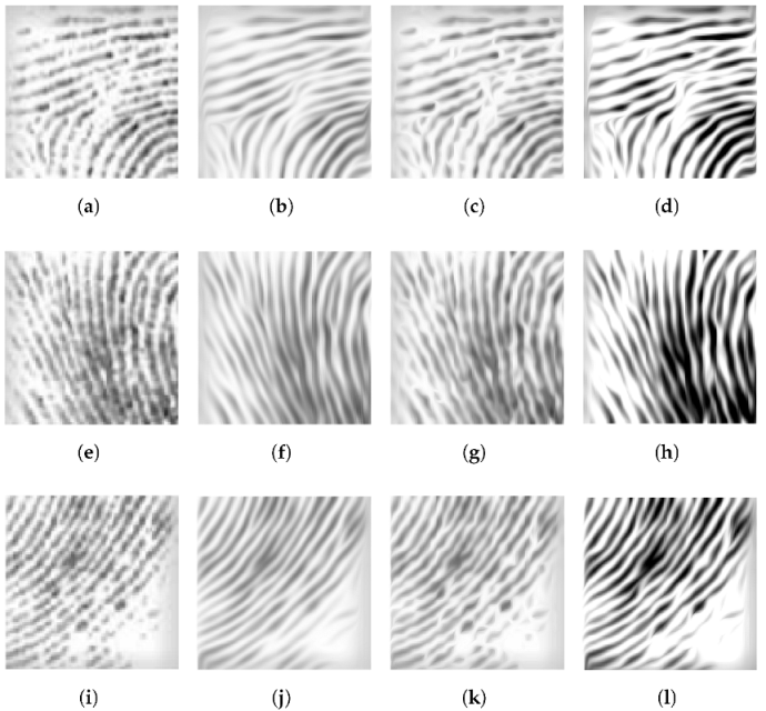
In this experiment, the spiral fingerprint image is divided into 9 subfigures in the ratio of 3 × 3 , represented by the coordinates location ( x , y ) , x , y = 1 , 2 , 3 subfigure. Based on the experimental results of Figure 5, we select the position (1,1) subfigure, position (2,1) subfigure, and position (3,3) subfigure as examples for demonstration. The experimental results are shown in Figure 6, and the parameter settings are the same as those in Figure 5.
Observing Figure 5d and Figure 6d, it is found that there are very short lines in the upper right corner of the “position (1,1) subfigure” of the original image. Observing Figure 5d and Figure 6e, it is found that there is a large gap in the left part of the “position (2,1) subfigure” of the original image, which is manifested by only leaving very short fingerprints similar to points. In Figure 6d,h, the corresponding positions of the subgraphs are restored, and the lines are clearer and more distinct. Observing Figure 6l, it is found that after the contrast in the lower right corner of the “position (3,3) subfigure” of the original image is enhanced, the degree of the flattening of the lines with small gray values relative to Figure 5d is decreased. Experiments showed that subdividing the image, which involves local processing of the image and changing the source terms, can achieve better results. On the other hand, in response to the poor restoration effect of the lines in the lower right and upper left corners of the original spiral fingerprint image, we find that this is not a problem with the model itself but rather due to the large grayscale range of the image; the average of the entire image cannot reflect the characteristics of local regions.
To verify the sensitivity of the model to noise, Gaussian noise with a standard deviation of 50 is added to the dustpan-shaped fingerprint image. The experimental results of the fingerprint2 image without Gaussian noise and with Gaussian noise are observed as shown in Figure 7 and Figure 8.
As shown in Figure 7b,c, the CED model and the CDEs model can complete the interrupted lines, while significantly reducing the contrast between the texture and background. On the contrary, Figure 7d indicates that our model completes the connection of interrupted lines while enhancing the contrast. Looking at Figure 8b,c, it is found that the CED model and the CDEs model are sensitive to noise. Figure 8d shows that the proposed model completely removes noise, and the image restoration effect is very good. This indicates that the proposed model can remove noise while connecting the interrupted lines.
According to the numerical experiments of fingerprint1 and fingerprint2 without/ containing Gaussian noise, Table 4 gives their contrast and entropy of images enhanced by the CED model, CDEs model and OURS model.
Comparing the contrast of different models for the same image, it is found that the proposed model has the highest contrast, indicating that the proposed model effectively improves the contrast of the image and makes it clearer. At the same time, by comparing the information entropy of the same picture with that of different models, it is found that the information entropy of the proposed model is the smallest, which means that the proposed model effectively reduces the chaos of the picture and the image becomes more smooth. The data in the Table 4 use contrast and information entropy to quantitatively demonstrate the effectiveness of the model in enhancing image contrast. In Table 4, the best results are shown in bold face.
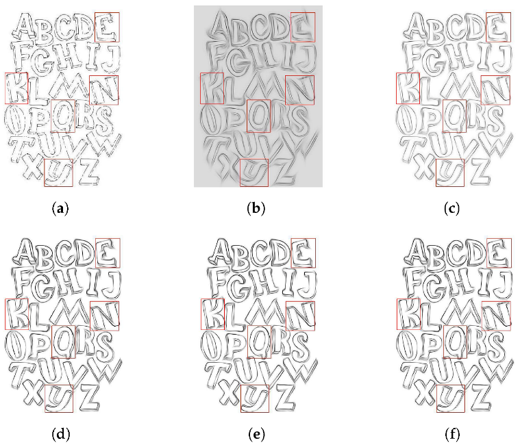
The following will conduct numerical experiments on two letter images and provide experimental results for different numerical formats of the CED model, CDEs model, and OURS model with different γ values, which are shown in Figure 9 and Figure 10.
The three pairs of local blocks shown in red line boxes in Figure 9 show that the proposed model can effectively restore blurry lines, successfully solving the problem of handwriting blurring caused by running out of ink or other reasons during writing. The letters “K, N, E, Q, Y” highlighted by the red lines in Figure 10 indicate that the proposed model achieved good connectivity for broken lines in the shapes of “horizontal, vertical, oblique, and arc”, and the restored image contrast is more pronounced. Figure 9d–f and Figure 10d–f show that different values of fractional-order γ can achieve the best recovery effect for the proposed model.
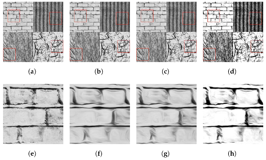
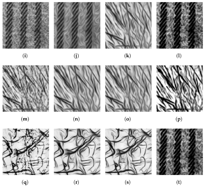
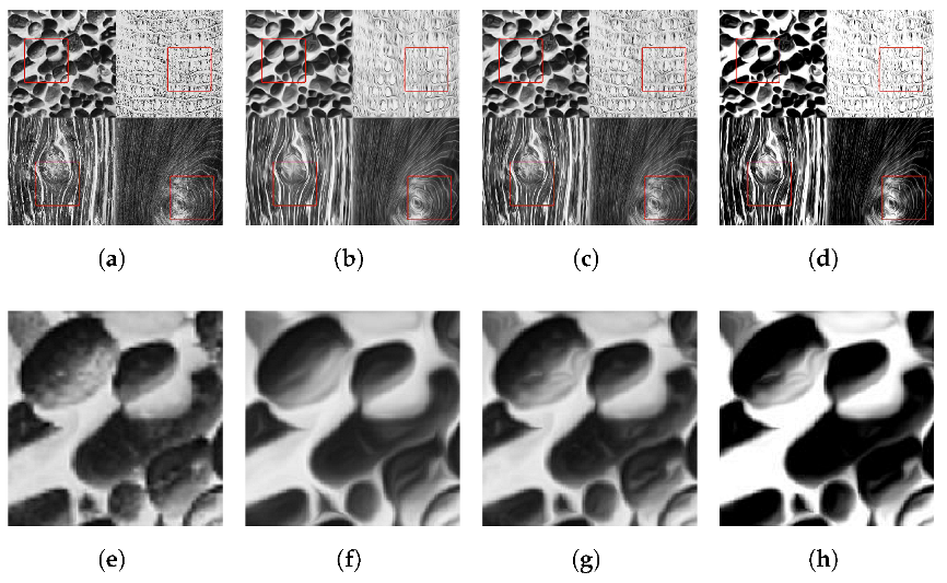
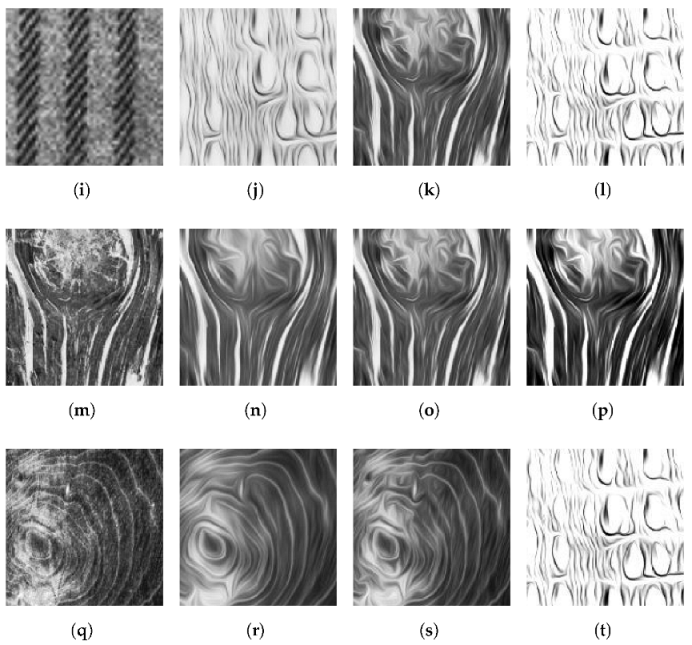
In order to observe the impact of the model on the shape and structure of “horizontal, vertical, oblique, and circular” in the text more intuitively, eight texture images are selected to synthesize two texture maps. Figure 11 and Figure 12 provide the processing results.
The typical “horizontal, vertical, oblique, and circular” shape structures in Figure 11 and Figure 12 have significantly enhanced the flow characteristics of the same type of line. The proposed model further deepens the flow characteristics of the same type of line. The four subimages in Texture1 exhibit the characteristics of spreading along the horizontal, vertical, oblique, and any direction, respectively. Figure 11e–t show the enlarged results of the four subimages in Texture 1. The four subimages in Texture 2 reflect the line features of circular, elliptical, and wavy structures. Figure 12e–t show the enlarged results of the four subimages in Texture 2. Compared with the CED model and CDEs model, the two images of the proposed model have a better enhancement effect, and the contrast of the images is greater, making the images clearer. The enhancement results of the two images further demonstrate the unified texture features of the images.
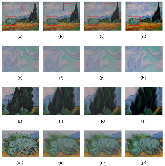
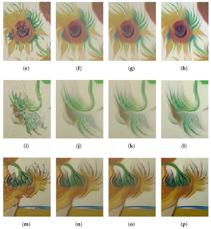
The proposed model is also applicable to color images, and the RGB channels of Van Gogh’s two oil paintings are enhanced separately, and then integrated to obtain the enhanced results.
Figure 13b–d and Figure 14b–d present the restoration results of two paintings under the CED model, CDEs model, and the proposed model. Figure 13e–p and Figure 14e–p, respectively, provide the restoration results of three enlarged images. Observing the cloud in Figure 13h, cypress in Figure 13l, and green plant in Figure 13p, as well as the sunflower with various poses in Figure 14p, it can be found that the proposed model restores the image lines, and the image contrast is more pronounced. Although Van Gogh’s works are not typical texture images, they still have characteristics similar to fluidity. As shown in Figure 13d and Figure 14d, the diffusion of the model further enhances the fluidity of the original image, and the image presents unity and coordination, reflecting the unified “texture scale” of the painting and Van Gogh’s unique painting style.
Numerical experiments show that, compared with the CED model and CDEs model, the proposed model can effectively not only connect blurred and interrupted lines but also enhance the contrast of images. In addition, the model can effectively remove noise. Experiments on grayscale and color image further illustrate that the model can deepen the fluidity characteristics of various types of lines. In the future, we can further develop other image enhancement methods based on the nonlinear structural tensor and try other numerical algorithms to improve the accuracy and efficiency of the algorithm.

4. Conclusions

In the framework of partial differential equations, we propose an image enhancement model based on fractional time-delay regularization and diffusion tensor for images with streamlined structures. The structural tensor is spatially regularization using nonlinear isotropic diffusion and is temporally regularized using fractional delay regularization, which makes the structural tensor nonlinear and stable. The proof of the existence and uniqueness of the solution theoretically ensures the feasibility of the model. Through numerical experiments on various streamlined images, the validity and feasibility of the model in this paper are verified.

Author Contributions

Conceptualization, W.Y. and Y.H.; methodology, all authors; software, Y.H. and W.Y.; validation, Z.Z. and B.W.; formal analysis, W.Y. and B.W.; investigation, Y.H. and W.Y.; resources, Z.Z. and B.W.; data curation, W.Y. and Y.H.; writing—original draft preparation, W.Y. and Y.H.; writing—review and editing, W.Y., Z.Z. and B.W.; visualization, Y.H. and W.Y.; supervision, Z.Z. and B.W.; project administration, Z.Z. and B.W.; funding acquisition, W.Y., Z.Z. and B.W. All authors have read and agreed to the published version of the manuscript.

Funding

This research was funded by the National Natural Science Foundation of China (11971131, 12171123, 61873071, 51476047, 11871133, 12271130, U21B2075), the Fundamental Research Funds for the Central Universities (HIT.NSRIF202202, 2022FRFK060014, 2022FRFK060020), China Postdoctoral Science Foundation (2020M670893), Natural Sciences Foundation of Heilongjiang Province (LH2022A011), and the China Society of Industrial and Applied Mathematics Young Women Applied Mathematics Support Research Project.

Data Availability Statement

The data used to support the findings of this study are available from the corresponding author upon request.

Conflicts of Interest

The authors declare no conflict of interest.

References

  1. Zou, G.; Li, T.; Li, G.; Peng, X.; Fu, G. A visual detection method of tile surface defects based on spatial-frequency domain image enhancement and region growing. In Proceedings of the 2019 Chinese Automation Congress (CAC), Hangzhou, China, 22–24 November 2019; pp. 1631–1636. [Google Scholar]
  2. Bhandari, A.K. A logarithmic law based histogram modification scheme for naturalness image contrast enhancement. J. Ambient. Intell. Humaniz. Comput. 2020, 11, 1605–1627. [Google Scholar] [CrossRef]
  3. Yu, T.; Zhu, M. Image enhancement algorithm based on image spatial domain segmentation. Comput. Inform. 2021, 40, 1398–1421. [Google Scholar] [CrossRef]
  4. Zhao, J.; Fang, Q. Noise reduction and enhancement processing method of cement concrete pavement image based on frequency domain filtering and small world network. In Proceedings of the 2022 International Conference on Edge Computing and Applications (ICECAA), Tamilnadu, India, 13–15 October 2022; pp. 777–780. [Google Scholar]
  5. Fabbri, C.; Islam, M.J.; Sattar, J. Enhancing underwater imagery using generative adversarial networks. In Proceedings of the 2018 IEEE International Conference on Robotics and Automation (ICRA), Brisbane, Australia, 12–15 May 2018; pp. 7159–7165. [Google Scholar]
  6. Huang, J.; Zhu, P.; Geng, M.; Ran, J.; Zhou, X.; Xing, C.; Wan, P.; Ji, X. Range scaling global u-net for perceptual image enhancement on mobile devices. In Proceedings of the European Conference on Computer Vision (ECCV) Workshops, Munich, Germany, 8–14 September 2018. [Google Scholar]
  7. Gabor, D. Information theory in electron microscopy. Lab. Investig. J. Tech. Methods Pathol. 1965, 14, 801–807. [Google Scholar]
  8. Jain, A.K. Partial differential equations and finite-difference methods in image processing, Part 1: Image represent. J. Optim. Theory Appl. 1977, 23, 65–91. [Google Scholar] [CrossRef]
  9. Perona, P.; Malik, J. Scale-space and edge detection using anisotropic diffusion. IEEE Trans. Pattern Anal. Mach. Intell. 1990, 12, 629–639. [Google Scholar] [CrossRef] [Green Version]
  10. Nitzberg, M.; Shiota, T. Nonlinear image filtering with edge and corner enhancement. IEEE Trans. Pattern Anal. Mach. Intell. 1992, 14, 826–833. [Google Scholar] [CrossRef]
  11. Cottet, G.H.; Germain, L. Image processing through reaction combined with nonlinear diffusion. Math. Comput. 1993, 61, 659–673. [Google Scholar] [CrossRef]
  12. Hao, Y.; Yuan, C. Fingerprint image enhancement based on nonlinear anisotropic reverse-diffusion equations. In Proceedings of the 26th Annual International Conference of the IEEE Engineering in Medicine and Biology Society, San Francisco, CA, USA, 1–5 September 2004; Volume 1, pp. 1601–1604. [Google Scholar]
  13. Brox, T.; Weickert, J.; Burgeth, B.; Mrázek, P. Nonlinear structure tensors. Image Vis. Comput. 2006, 24, 41–55. [Google Scholar] [CrossRef] [Green Version]
  14. Wang, W.W.; Feng, X.C. Anisotropic diffusion with nonlinear structure tensor. Multiscale Model. Simul. 2008, 7, 963–977. [Google Scholar] [CrossRef]
  15. Marin-McGee, M.J.; Velez-Reyes, M. A spectrally weighted structure tensor for hyperspectral imagery. IEEE J. Sel. Top. Appl. Earth Obs. And Remote Sens. 2016, 9, 4442–4449. [Google Scholar] [CrossRef]
  16. Marin-McGee, M.; Velez-Reyes, M. Coherence enhancement diffusion for hyperspectral imagery using a spectrally weighted structure tensor. In Proceedings of the 2016 8th Workshop on Hyperspectral Image and Signal Processing: Evolution in Remote Sensing (WHISPERS), Los Angeles, CA, USA, 21–24 August 2016; pp. 1–4. [Google Scholar]
  17. Nnolim, U.A. Partial differential equation-based hazy image contrast enhancement. Comput. Electr. Eng. 2018, 72, 670–681. [Google Scholar] [CrossRef]
  18. Gu, Z.; Chen, Y.; Chen, Y.; Lu, Y. SAR image enhancement based on PM nonlinear diffusion and coherent enhancement diffusion. In Proceedings of the IGARSS 2020—2020 IEEE International Geoscience and Remote Sensing Symposium, Waikoloa, HI, USA, 26 September–2 October 2020; pp. 581–584. [Google Scholar]
  19. Bai, J.; Feng, X.C. Fractional-order anisotropic diffusion for image denoising. IEEE Trans. Image Process. 2007, 16, 2492–2502. [Google Scholar] [CrossRef] [PubMed]
  20. Sharma, D.; Chandra, S.K.; Bajpai, M.K. Image enhancement using fractional partial differential equation. In Proceedings of the 2019 Second International Conference on Advanced Computational and Communication Paradigms (ICACCP), Gangtok, India, 25–28 February 2019; pp. 1–6. [Google Scholar]
  21. Chandra, S.K.; Bajpai, M.K. Fractional mesh-free linear diffusion method for image enhancement and segmentation for automatic tumor classification. Biomed. Signal Process. Control 2020, 58, 101841. [Google Scholar] [CrossRef]
  22. Nnolim, U.A. Forward-reverse fractional and fuzzy logic augmented partial differential equation-based enhancement and thresholding for degraded document images. Optik 2022, 260, 169050. [Google Scholar] [CrossRef]
  23. Ben-loghfyry, A. Reaction-diffusion equation based on fractional-time anisotropic diffusion for textured images recovery. Int. J. Appl. Comput. Math. 2022, 8, 177. [Google Scholar] [CrossRef]
  24. Weickert, J. Coherence-enhancing diffusion filtering. Int. J. Comput. Vis. 1999, 31, 111. [Google Scholar] [CrossRef]
  25. Chen, Y.; Levine, S. Image recovery via diffusion tensor and time-delay regularization. J. Vis. Commun. Image Represent. 2002, 13, 156–175. [Google Scholar] [CrossRef] [Green Version]
  26. Cottet, G.; Ayyadi, M.E. A Volterra type model for image processing. IEEE Trans. Image Process. 1998, 7, 292–303. [Google Scholar] [CrossRef] [Green Version]
  27. Koeller, R. Applications of fractional calculus to the theory of viscoelasticity. Trans. ASME J. Appl. Mech. 1984, 51, 299–307. [Google Scholar] [CrossRef]
  28. Benson, D.A.; Wheatcraft, S.W.; Meerschaert, M.M. Application of a fractional advection-dispersion equation. Water Resour. Res. 2000, 36, 1403–1412. [Google Scholar] [CrossRef] [Green Version]
  29. Butzer, P.L.; Westphal, U. An introduction to fractional calculus. In Applications of Fractional Calculus in Physics; World Scientific: Singapore, 2000; pp. 1–85. [Google Scholar]
  30. Dou, F.; Hon, Y. Numerical computation for backward time-fractional diffusion equation. Eng. Anal. Bound. Elem. 2014, 40, 138–146. [Google Scholar] [CrossRef]
  31. Cuesta-Montero, E.; Finat, J. Image processing by means of a linear integro-differential equation. In Proceedings of the 3rd IASTED International Conference on Visualization, Imaging, and Image Processing, Benalmadena, Spain, 8–10 September 2003; Volume 1. [Google Scholar]
  32. Janev, M.; Pilipović, S.; Atanacković, T.; Obradović, R.; Ralević, N. Fully fractional anisotropic diffusion for image denoising. Math. Comput. Model. 2011, 54, 729–741. [Google Scholar] [CrossRef]
  33. Li, Y.; Liu, F.; Turner, I.W.; Li, T. Time-fractional diffusion equation for signal smoothing. Appl. Math. Comput. 2018, 326, 108–116. [Google Scholar] [CrossRef] [Green Version]
  34. Li, L.; Liu, J.G. Some compactness criteria for weak solutions of time fractional PDEs. SIAM J. Math. Anal. 2018, 50, 3963–3995. [Google Scholar] [CrossRef] [Green Version]
  35. Li, L.; Liu, J.G. A generalized definition of Caputo derivatives and its application to fractional ODEs. SIAM J. Math. Anal. 2018, 50, 2867–2900. [Google Scholar] [CrossRef] [Green Version]
  36. Alikhanov, A. A priori estimates for solutions of boundary value problems for fractional-order equations. Differ. Equ. 2010, 46, 660–666. [Google Scholar] [CrossRef] [Green Version]
  37. Agrawal, O. Fractional variational calculus in terms of Riesz fractional derivatives. J. Phys. A Math. Theor. 2007, 40, 6287. [Google Scholar] [CrossRef]
  38. Dong, G.; Guo, Z.; Zhou, Z.; Zhang, D.; Wo, B. Coherence-enhancing diffusion with the source term. Appl. Math. Model. 2015, 39, 6060–6072. [Google Scholar] [CrossRef]
  39. Evans, L.C. Partial Differential Equations; American Mathematical Society: Providence, RI, USA, 2022; Volume 19. [Google Scholar]
  40. Suri, J.S.; Laxminarayan, S. PDE and Level Sets; Springer Science & Business Media: New York, NY, USA, 2002. [Google Scholar]
  41. Murio, D.A. Implicit finite difference approximation for time fractional diffusion equations. Comput. Math. Appl. 2008, 56, 1138–1145. [Google Scholar] [CrossRef]
  42. Weickert, J.; Scharr, H. A scheme for coherence-enhancing diffusion filtering with optimized rotation invariance. J. Vis. Commun. Image Represent. 2002, 13, 103–118. [Google Scholar] [CrossRef] [Green Version]
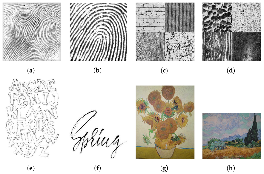
Figure 1. Test figures: (a) fingerprint1; (b) fingerprint2; (c) texture1; (d) texture2; (e) alphabet; (f) spring; (g) sunflowers; (h) cypress.
Fractalfract 07 00569 g001
Figure 2. Different values of λ in the proposed model: (a) fingerprint1; (b) λ = 1.8 × 10 3 ; (c) λ = 1.8 × 10 1 ; (d) λ = 1.8 .
Fractalfract 07 00569 g002
Figure 3. Different values of τ in the proposed model: (a) τ = 5 × 10 3 ; (b) τ = 5 × 10 1 ; (c) τ = 5 × 10 4 ; (d) τ = 5 × 10 5 .
Fractalfract 07 00569 g003
Figure 4. Different values of γ in the proposed model: (a) γ = 0.3 ; (b) γ = 0.5 ; (c) γ = 0.7 ; (d) γ = 0.9 .
Fractalfract 07 00569 g004
Figure 5. Fingerprint1 image: (a) original image; (b) results obtained by CED; (c) results obtained by CDEs; (d) results obtained by OURS.
Fractalfract 07 00569 g005
Figure 6. Experimental results of fingerprint1 with subfigures of “positions (1,1), (2,1), and (3,3)”: (a) (1,1) original subfigure; (b) (1,1) results obtained by CED; (c) (1,1) results obtained by CDEs; (d) (1,1) results obtained by OURS; (e) (2,1) original subfigure; (f) (2,1) results obtained by CED; (g) (2,1) results obtained by CDEs; (h) (2,1) results obtained by OURS; (i) (3,3) original subfigure; (j) (3,3) results obtained by CED; (k) (3,3) results obtained by CDEs; (l) (3,3) results obtained by OURS.
Fractalfract 07 00569 g006
Figure 7. Fingerprint2 image without noise: (a) original image; (b) results obtained by CED; (c) results obtained by CDEs; (d) results obtained by OURS.
Fractalfract 07 00569 g007
Figure 8. Fingerprint2 image with noise: (a) original image; (b) results obtained by CED; (c) results obtained by CDEs; (d) results obtained by OURS.
Fractalfract 07 00569 g008
Figure 9. Spring image: (a) original image; (b) results obtained by CED; (c) results obtained by CDEs; (d) results obtained by OURS with γ = 0.1 ; (e) results obtained by OURS with γ = 0.5 ; (f) results obtained by OURS with γ = 0.7 .
Fractalfract 07 00569 g009
Figure 10. Alphabet image: (a) original image; (b) results obtained by CED; (c) results obtained by CDEs; (d) results obtained by OURS with γ = 0.1 ; (e) results obtained by OURS with γ = 0.5 ; (f) results obtained by OURS with γ = 0.7 .
Fractalfract 07 00569 g010
Figure 11. Texture1 image: (a) original image; (b) results obtained by CED; (c) results obtained by CDEs; (d) results obtained by OURS; (e)/(i)/(m)/(q) enlarged image 01/02/03/04; (f)/(j)/ (n)/(r) enlarged image 01/02/03/04 by CED; (g)/(k)/(o)/(s) enlarged image 01/02/03/04 by CDEs; (h)/(l)/(p)/(t) enlarged image 01/02/03/04 by OURS.
Fractalfract 07 00569 g011aFractalfract 07 00569 g011b
Figure 12. Texture2 image: (a) Original image; (b) results obtained by CED; (c) results obtained by CDEs (d) results obtained by OURS; (e)/(i)/(m)/(q) enlarged image 01/02/03/04; (f)/(j)/(n)/(r) enlarged image 01/02/03/04 by CED; (g)/(k)/(o)/(s) enlarged image 01/02/03/04 by CDEs; (h)/(l)/(p)/(t) enlarged image 01/02/03/04 by OURS.
Fractalfract 07 00569 g012aFractalfract 07 00569 g012b
Figure 13. Cypress image: (a) Original image; (b) results obtained by CED; (c) results obtained by CDEs (d) results obtained by OURS; (e)/(i)/(m) enlarged image 01/02/03; (f)/(j)/(n) enlarged image 01/02/03 by CED; (g)/(k)/(o) enlarged image 01/02/03 by CDEs; (h)/(l)/(p) enlarged image 01/02/03 by OURS.
Fractalfract 07 00569 g013
Figure 14. Sunflowers image: (a) original image; (b) results obtained by CED; (c) results obtained by CDEs; (d) results obtained by OURS; (e)/(i)/(m) enlarged image 01/02/03; (f)/(j)/(n) enlarged image 01/02/03 by CED; (g)/(k)/(o) enlarged image 01/02/03 by CDEs; (h)/(l)/(p) enlarged image 01/02/03 by OURS.
Fractalfract 07 00569 g014aFractalfract 07 00569 g014b
Table 1. This is the parameter selection in CED model experiment.
Test Figures σ ρ t ced Iter CED
fingerprint10.340.3100
fingerprint20.540.5100
spring0.550.280
alphabet0.360.3150
texture10.350.5100
texture20.370.5150
sunflower0.220.650
cypress0.220.650
Table 2. This is the parameter selection in CDEs model experiment.
Test Figures σ t 1 cdes t 2 cdes Iter CDEs
fingerprint10.50.20.330
fingerprint20.50.20.5100
spring0.30.10.250
alphabet0.30.150.390
texture10.50.150.5110
texture20.50.20.5100
sunflower0.20.20.630
cypress0.20.20.630
Table 3. This is the parameter selection in our model experiment.
Test Figures σ λ τ γ Δ t Δ t Iter OURS
fingerprint10.50.0180.50.70.20.3120
fingerprint20.50.0180.50.70.20.5100
spring0.30.020.5(0.1, 0.5, 0.7)0.10.240
alphabet0.50.0250.3(0.1, 0.5, 0.7)0.150.380
texture10.50.020.50.70.150.560
texture20.50.0070.50.10.20.5150
sunflower0.20.020.50.50.20.630
cypress0.20.020.50.50.20.630
Table 4. Contrast and information entropy of two fingerprint images with respect to different models.
Figure 5Figure 5Figure 7Figure 7Figure 8Figure 8
contrastentropycontrastentropycontrastentropy
original43.597.2480.316.6281.396.74
CED35.277.1571.187.2771.317.25
CDEs--71.957.2875.697.15
OURS73.576.49113.563.75119.133.05
Disclaimer/Publisher’s Note: The statements, opinions and data contained in all publications are solely those of the individual author(s) and contributor(s) and not of MDPI and/or the editor(s). MDPI and/or the editor(s) disclaim responsibility for any injury to people or property resulting from any ideas, methods, instructions or products referred to in the content.