Article

The Improved Stochastic Fractional Order Gradient Descent Algorithm

1
School of Mathematics and Statistics, Beijing Technology and Business University, Beijing 100048, China
2
School of Future Technology, Beijing Technology and Business University, Beijing 100048, China
3
School of Artificial Intelligence and Electrical Engineering, Guizhou Institute of Technology, Special Key Laboratory of Artificial Intelligence and Intelligent Control of Guizhou Province, Guiyang 550003, China
*
Author to whom correspondence should be addressed.
Fractal Fract. 2023, 7(8), 631; https://doi.org/10.3390/fractalfract7080631
Submission received: 17 July 2023 / Revised: 11 August 2023 / Accepted: 16 August 2023 / Published: 18 August 2023
(This article belongs to the Special Issue Optimal Control Problems for Fractional Differential Equations)

Abstract

:
This paper mainly proposes some improved stochastic gradient descent (SGD) algorithms with a fractional order gradient for the online optimization problem. For three scenarios, including standard learning rate, adaptive gradient learning rate, and momentum learning rate, three new SGD algorithms are designed combining a fractional order gradient and it is shown that the corresponding regret functions are convergent at a sub-linear rate. Then we discuss the impact of the fractional order on the convergence and monotonicity and prove that the better performance can be obtained by adjusting the order of the fractional gradient. Finally, several practical examples are given to verify the superiority and validity of the proposed algorithm.

1. Introduction

In the field of machine learning, the gradient descent algorithm is one of the most fundamental methods for optimization problems [1,2]. Due to the continuous expansion of the scale of data, the traditional gradient descent algorithms cannot be used effectively to solve the optimization problems in large-scale machine learning [3,4,5]. To deal with this situation, the SGD algorithm was introduced, which is an online optimization algorithm and can be used to reduce the computational complexity by selecting one or several sample gradients randomly to replace the overall gradients in the iteration process [6]. Recently, to improve performance, the traditional SGD algorithm was modified from the different aspects, such as the adaptive gradient algorithm (Adagrad) [7], the Adadelta method [8] and adaptive moment estimation (Adam) [9], where the objective functions were assumed to be convex or strongly convex, which might be not satisfied in applications. Hence, the nonconvex learning algorithm was introduced [10].
In some practical problems, the bounds of the regret need to be minimized as far as possible. Hence, a fractional order gradient was introduced due to its good properties, such as long memory and multiple parameters [11,12]. However, the fractional order algorithm might fail to find the optimum [13]. Hence, some improved fractional order gradient algorithms were proposed by the technology of the truncation of high order terms [14,15,16]. By using a variable initial value strategy and truncation on high order terms, the fractional order gradient descent method was transformed into an adaptive learning rate method, the learning rate of which corresponds to the power of the previous terms. Its long memory property was transformed into a short memory property that can be tolerated. By combining the SGD algorithm and fractional order, some composite algorithms were introduced in machine learning [17,18,19,20,21]. However, the literature above only applied new algorithms with a fractional order gradient to applications without proving its convergence or proving its convergence on a rather specific algorithm, like an RBF neural network; to the best of our knowledge, there are few theoretical works on general fractional online SGD algorithms.
In this paper, we mainly propose three new SGD algorithms with a fractional order gradient for the online optimization problem, under which the bounds of the regret can be lowered by adjusting the fractional order. The main contributions of this paper include the following three aspects.
(1) Three improved stochastic fractional order gradient algorithms are proposed for the online optimization problem combing fractional gradients.
(2) Compared with the results in [20,21], where only simulation results were expressed, this paper proves the convergence of the proposed algorithms in mathematics. In addition, it is shown that the fractional order gradient can relieve the gradient exploding phenomenon, which often occurs in deep learning.
(3) The proposed algorithms are applied to the parameter identification problem and the classification problem to examine the effectiveness of the proposed algorithm.
Notation 1.
Let R n be the Euclidean space with dimension n. N is the natural number of a set, given A R n × m and x R n , A and x are the 2-norm, and | x | is the absolute value vector of each component of x. f ( x ) denotes the gradient of f ( x ) .

2. Materials and Methods

Many researchers have given different definitions of a fractional derivate from different aspects; the Caputo type is the most common in applications due to its integer order initial values condition. Additionally, the Riemann—Liouville type also works in some situations [14]. For a smooth function f ( t ) , the Caputo derivate is defined by
t 0 C D t α f ( t ) = 1 Γ ( n α ) t 0 t f ( n ) ( τ ) ( t τ ) α n + 1 d τ ,
where n 1 < α < n , n N , and Formula (1) can be rewritten in Taylor series as follows:
t 0 C D t α f ( t ) = i = 1 f ( i ) ( t 0 ) Γ ( i + 1 α ) ( t t 0 ) i α , 0 < α < 1 .
Let f ( θ ) be a convex objective function, and the traditional gradient descent algorithm is
θ t + 1 = θ t μ t g t ,
where g t = f ( θ t ) and μ t is the learning rate. Substituting the gradient by the fractional order gradient in (3), we get the following iteration algorithm:
θ t + 1 = θ t μ t θ 0 C D θ t α f ( θ t ) .
To eliminate the effect of the global character of a fractional differential operator, we choose the following variable initial value strategy, i.e.,
θ t + 2 = θ t + 1 μ t θ t C D θ t + 1 α f ( θ t ) .
Adopting the Tayor series of a fractional order differential, we have
θ t + 2 = θ t + 1 μ t i = 0 f ( i + 1 ) ( θ t ) Γ ( i + 2 α ) ( θ t + 1 θ t ) i + 1 α , 0 < α < 1 .
By Reserving the first item and omitting the other items in the summation, we have
θ t + 2 = θ t + 1 μ t f ( θ t + 1 ) Γ ( 2 α ) ( θ t + 1 θ t ) 1 α .
In fact, we can extend algorithm (7) to the case of 1 < α < 2 directly. In the following, we assume 0 < α < 2 . To guarantee the feasibility of ( θ t + 1 θ t ) 1 α , we modify (7) into the following form:
θ t + 2 = θ t + 1 μ t f ( θ t + 1 ) Γ ( 2 α ) | θ t + 1 θ t | 1 α .
Remark 1.
Notice the properties of the gamma function—singularities would occur when the orders of the fractional gradient are taken as other integers α = 3 , 4 , . And the gamma function displays a poor property when the order is closed to its singularities.
For the SGD algorithm, each batch of samples has its own objective function f t ( θ ) . The task of this paper is to propose the SGD algorithm with a fractional order and analyze their convergence.
Let
R ( T ) = t = 1 T f t ( θ t ) m i n θ t = 1 T f t ( θ ) ,
where R ( T ) is the empirical regret function of the optimization problem and f t ( θ ) is the objective sub-function of one batch of samples at present. If R ( T ) / T 0 as T , then we call that algorithm convergent. Next, we will analyze the asymptotic property of R ( T ) ,
R ( T ) = t = 1 T f t ( θ t ) m i n θ t = 1 T f t ( θ t ) = t = 1 T f t ( θ t ) t = 1 T f t ( θ * ) = t = 1 T [ f t ( θ t ) f t ( θ * ) ] ,
where θ * a r g m i n θ t = 1 T f t ( θ ) . We need the following assumptions on parameter space and objective functions in the following analysis [22].
Assumption 1.
Suppose all f i ( θ ) are convex. By using the property of the convex function, we conclude that f ( w ) f ( v ) g , w v , where g = f ( v ) .
Assumption 2.
Suppose that parameters θ * θ d and θ i θ j D , θ i , θ j θ n , where θ d is a bounded and closed set and D > 0 is a positive scalar.
Assumption 3.
Suppose the gradient of the objective function is bounded, i.e., g t G , t , where g t is the gradient of function f t in the tth batch of data.
Remark 2.
In Assumption 1, we assume all objective functions f t ( θ ) are convex. Hence, there must exist a global optimal parameter for the objective function. Assumption 2 implies that the Euclidean distance of any two temporary parameters would not be too long. Most of the results on online optimization require this assumption, because the optimal points of different objective functions can be far apart. Assumption 3 guarantees that the gradient of the objective function is bounded, which is very important for minimizing the empirical regret function [23]. When parameters between iterations are bounded, it can be proved that the gradient is also bounded since the objective function cannot vary too severely during a bounded interval. An example is Gaussian kernel function f ( x ) = e x p ( x 2 ) . In addition, in machine learning, Assumption 3 can also be satisfied by clipping the gradient [24].

3. Main Results

In this section, we will analyze the convergence of the proposed three online algorithms with fractional order α .

3.1. Standard SGD with Fractional Order Gradient

θ t + 2 = θ t + 1 μ t f ( θ t + 1 ) Γ ( 2 α ) ( | θ t + 1 θ t | + δ ) 1 α .
To avoid the phenomena that the before and after iteration values are the same, we add a small positive parameter δ to the format of the algorithm to improve the performance.
Theorem 1.
Under Assumptions 1–3, Algorithm 1 is convergent, and the bound of R ( T ) can be adjusted by fractional order α .
Proof. 
By Formula (10), we have
θ t + 1 θ * = θ t θ * μ t α f t ( θ t ) θ t + 1 θ * = θ t θ * μ t Γ ( 2 α ) g t ( | θ t θ t 1 | + δ ) 1 α θ t + 1 θ * 2 = θ t θ * μ t Γ ( 2 α ) g t ( | θ t θ t 1 | + δ ) 1 α 2 .
Then,
g t , θ t θ * = Γ ( 2 α ) 2 μ t θ t + 1 θ * 2 θ t θ * 2 | θ t θ t 1 | + δ 1 α + μ t 2 Γ ( 2 α ) g t 2 | θ t θ t 1 | + δ 1 α .
By applying the property of convex objective function f t ( θ t ) f t ( θ * ) g t , θ * θ t and the definition of R(T), we have R ( T ) t = 1 T g t , θ * θ t . Together with (11), we have
R ( T ) t = 1 T Γ ( 2 α ) 2 μ t θ t + 1 θ * 2 θ t θ * 2 | θ t θ t 1 | + δ 1 α + t = 1 T μ t 2 Γ ( 2 α ) g t 2 | θ t θ t 1 | + δ 1 α .
The first summation term of (12) can be enlarged by rearranging the order of the term as follows:
t = 1 T Γ ( 2 α ) 2 μ t θ t + 1 θ * 2 θ t θ * 2 | θ t θ t 1 | + δ 1 α Γ ( 2 α ) δ α 1 2 [ θ 1 θ * 2 μ 1 + t = 2 T ( 1 μ t 1 μ t 1 ) θ t θ * 2 2 θ T + 1 θ * 2 2 μ T ] Γ ( 2 α ) δ α 1 2 [ 1 μ 1 D 2 + D 2 t = 2 T ( 1 μ t 1 μ t 1 ) + 0 ] Γ ( 2 α ) D 2 δ α 1 2 μ T .
By adopting Assumption 3, we can get the bounds of the regret function from different situations.
When fractional order 0 < α 1 :
R ( T ) D 2 δ α 1 2 μ T + t = 1 T μ t 2 g t 2 θ t θ t 1 + δ 1 α D 2 δ α 1 Γ ( 2 α ) 2 μ T + G 2 ( D + δ ) 1 α 2 Γ ( 2 α ) t = 1 T μ t .
When fractional order 1 < α < 2 :
R ( T ) D 2 ( D + δ ) α 1 Γ ( 2 α ) 2 μ T + t = 1 T μ t 2 Γ ( 2 α ) g t 2 | θ t θ t 1 | + δ 1 α D 2 ( D + δ ) α 1 Γ ( 2 α ) 2 μ T + G 2 δ 1 α 2 Γ ( 2 α ) t = 1 T μ t .
And the bounds of the regret function on 0 < α < 2 can be summarized as
R ( T ) D 2 δ α 1 Γ ( 2 α ) 2 μ T + G 2 ( D + δ ) 1 α 2 Γ ( 2 α ) t = 1 T μ t , 0 < α 1 , D 2 ( D + δ ) α 1 Γ ( 2 α ) 2 μ T + G 2 δ 1 α 2 Γ ( 2 α ) t = 1 T μ t , 1 < α < 2 .
Let T ; the convergence of Algorithm 1 is decided by 1 μ T T and t = 1 T μ t T . When we take the polynomial decay rate, such as μ t = C t p , p 0 , especially when p = 1 2 , R ( T ) obtains its optimal bound O ( T ) for 1 μ T T = C T and t = 1 T C t 1 + 1 T d t t = 2 T 1 . Therefore, R ( T ) / T = O ( 1 T ) 0 ; hence, Algorithm 1 is convergent.    □
Algorithm 1 SGD with fractional order.
1:
Initialize α , μ 0 , t m a x , t = 0 and θ 0 ;
2:
Calculate θ 1 under ordinary SGD: θ 1 = θ 0 μ 0 f 0 ( θ 0 ) ;
3:
Update the parameters by θ t + 2 = θ t + 1 μ t + 1 f ( θ t + 1 ) Γ ( 2 α ) ( | θ t + 1 θ t | + δ ) 1 α and μ t = μ 0 t ;
4:
Increase t to t m a x until all batches of samples have been used.
Remark 3.
Compared with the integer order algorithm, fractional term ( | θ t + 1 θ t | + δ ) 1 α Γ ( 2 α ) would accelerate the convergence of algorithms. When 0 < α 1 , a larger value of fractional term ( | θ t + 1 θ t | + δ ) 1 α Γ ( 2 α ) leads to an increase in learning rate when θ t + 1 and θ t differ significantly and the difference is close to D at the beginning of iterations; the situation is the opposite when 1 < α < 2 . In particular, when D < 0.5 , D 1 α Γ ( 2 α ) is an incremental function of 0 < α < 1.5 .
Remark 4.
When learning rate μ t = μ 0 / t p , R ( T ) = O ( T m a x ( p , 1 p ) ) . And if we take μ t as a constant, R ( T ) / T = O ( 1 ) , the algorithm still works for other some situations in [20,25].
Remark 5.
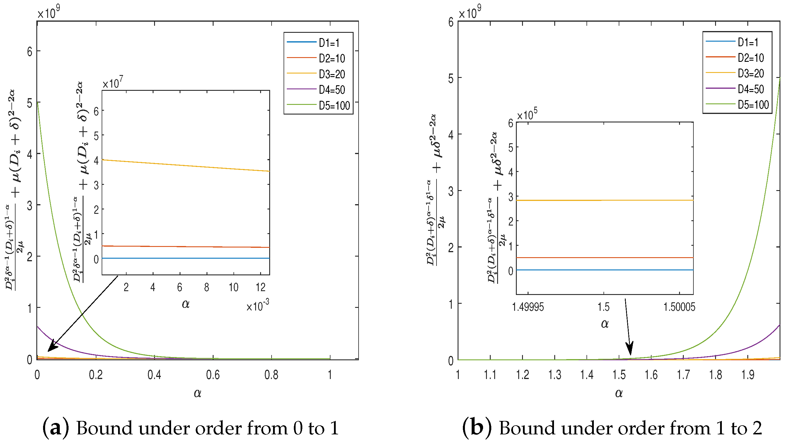
The bound of the regret function mainly depends on the summation part of Formula (16). When we take parameters δ = 10 3 and D in the algorithm of different orders, we find that the monotonicity of the regret function would vary as a fractional order. It is shown that the larger fractional order brings a smaller loss of function when 0 < α 1 , while the result is the opposite when 1 < α < 2 until the order is close to 2. We usually take the normalization of the training data to reduce the effect of data magnitude. Hence, the value of D used in Figure 1 is meaningful where the monotonicity of the coefficient is shown in Figure 1.

3.2. Adagrad Algorithm with Fractional Order

Notation 2.
For the Adagrad algorithm with a fractional order, we need to split parameters and variables by its dimension as θ t = [ θ t , 1 , , θ t , d ] T , g t = [ g t , 1 , , g t , d ] T and μ t = [ μ t , 1 , , μ t , n ] T .
Theorem 2.
Under Assumptions 1–3, Algorithm 2 is convergent, where · is the Hadamard product between vectors and μ is a constant.
Proof. 
We split the objective function according to its dimension:
t = 1 T g t , θ t θ * = t = 1 T i = 1 d g t , i ( θ t , i θ i * ) = i = 1 d t = 1 T g t , i ( θ t , i θ i * ) .
We get the same form of R ( T ) with Theorem 1 when 0 < α 1 :
R ( T ) i = 1 d [ t = 1 T Γ ( 2 α ) 2 μ t , i ( θ t , i θ i * ) 2 ( θ t + 1 , i θ i * ) 2 ( θ t + 1 , i θ t , i ) 1 α + t = 1 T μ t , i 2 Γ ( 2 α ) g t , i 2 ( θ t + 1 , i θ t , i ) 1 α ] ;
hence,
R ( T ) i = 1 d [ D i 2 δ α 1 2 μ s = 1 T g s , i 2 θ s , i θ s 1 , i 2 2 α + μ ( D i + δ ) 1 α 2 i = 1 T g t , i 2 g s , i 2 θ s , i θ s 1 , i 2 2 α ] .
The first term of Formula (19) can be enlarged to
s = 1 T g s , i 2 θ s , i θ s 1 , i 2 2 α G i D i 1 α T .
For the last term, we have
t = 1 T g t , i 2 ( | θ t , i θ t 1 , i | + δ ) 2 2 α s = 1 t g s , i 2 ( θ s , i θ s 1 , i ) 2 2 α = t = 1 T 2 g t , i 2 ( | θ t , i θ t 1 , i | + δ ) 2 2 α s = 1 t g s , i 2 ( θ s , i θ s 1 , i ) 2 2 α + s = 1 t g s , i 2 ( θ s , i θ s 1 , i ) 2 2 α g 1 , i 2 ( | θ 1 , i θ 0 , i | + δ ) 2 2 α g 1 , i 2 ( θ 1 , i θ 0 , i ) 2 2 α + t = 2 T 2 g t , i 2 ( | θ t , i θ t 1 , i | + δ ) 2 2 α s = 1 t g s , i 2 ( θ a , i θ a 1 , i ) 2 2 α + s = 1 t 1 g s , i 2 ( θ s , i θ s 1 , i ) 2 2 α g 1 , i 2 ( | θ 1 , i θ 0 , i | + δ ) 2 2 α + t = 2 T ( 2 s = 1 t g s , i 2 ( | θ s , i θ s 1 , i | + δ ) 2 2 α 2 s = 1 t 1 g s , i 2 ( | θ s , i θ s 1 , i | + δ ) 2 2 α ) 2 s = 1 T g s , i 2 ( | θ s , i θ s 1 , i | + δ ) 2 2 α 2 G i ( D + δ ) 1 α T .
Finally, combining Formula (21) and the estimation of the first term of R ( T ) , we have
R ( T ) i = 1 d [ D i 2 G i δ α 1 ( D i + δ ) 1 α 2 μ T ] + i = 1 d [ μ ( D i + δ ) 2 2 α G i T ] . = i = 1 d G i ( [ D i 2 δ α 1 ( D i + δ ) 1 α 2 μ + μ ( D i + δ ) 2 2 α ] T .
Similarly, we get the bound of R ( T ) when 1 < α < 2 :
R ( T ) i = 1 d G i ( [ D i 2 ( D i + δ ) α 1 δ 1 α 2 μ + μ δ 2 2 α ] T .
Similar to the proof in Theorem 1, let T , R ( T ) T = O ( 1 T ) 0 , which means Adagrad with fractional order is convergent.    □
Algorithm 2 Adagrad with fractional order.
1:
Initialize α , μ 0 , t m a x , t = 0 and θ 0 ;
2:
Calculate θ 1 under ordinary SGD: θ 1 = θ 0 μ 0 f 0 ( θ 0 ) ;
3:
Update the parameters by θ t + 1 = θ t μ t Γ ( 2 α ) · g t | θ t θ t 1 | + δ 1 α and μ t , i = μ Γ ( 2 α ) s = 1 t g s , i 2 θ s , i θ s 1 , i 2 2 α ;
4:
Increase t to t m a x until all batches of samples have been used.
Remark 6.
The learning rate of Algorithm 2 is related to its history gradient information. When the number of iterations is increasing, the value of the summation of the former gradient is hard to compute; meanwhile, the step size decreases so that new samples become less important. Once we take fractional order α into the algorithm, history gradient accumulation can be relieved by selecting a bigger order but the extra cost of the computation of the fractional gradient would increase.
Remark 7.
Different from Algorithm 1, the fractional gradient part of adaptive step size μ t does not need a parameter δ to avoid singularity due to the accumulation of the square of the history gradient. Actually, parameter δ might damage the convergence of the algorithm, especially when 1 < α < 2 as shown in Figure 2.

3.3. SGD with Momentum and Fractional Order Gradient

Theorem 3.
Under Assumptions 1–3, Algorithm 3 with momentum is convergent.
Algorithm 3 mSGD with fractional order
1:
Initialize α , μ 0 , β 0 , t m a x , t = 0 and θ 0 , m 0 = 0 ;
2:
Calculate θ 1 under ordinary SGD: θ 1 = θ 0 μ 0 f 0 ( θ 0 ) ;
3:
Update the parameters by θ t + 1 = θ t μ t m ^ t , m t = β t m t 1 + ( 1 β t ) g t | θ t θ t 1 | + δ 1 α Γ ( 2 α ) and m ^ t = m t 1 i = 1 t β i ; μ t + 1 = μ 0 t + 1 , β t + 1 = β 0 t + 1 ;
4:
Increase t to t m a x until all batches of samples have been used.
Proof. 
For simplicity, denote h t , i = g t , i ( | θ i , t θ i , t 1 | + δ ) 1 α Γ ( 2 α ) . The proposed algorithm can be expressed in the form of a component.
θ i , t + 1 = θ i , t μ t m ^ i , t = θ i , t μ t m i , t 1 i = 1 t β i = θ i , t μ t β t m i , t 1 + ( 1 β t ) h t , i 1 i = 1 t β i .
Similar to [9], we set β i c < 1 as a decreasing sequence which means momentum m i would be close to h i .
Let θ i , t + 1 = θ i , t μ t β t m i , t 1 + ( 1 β t ) h t , i 1 s = 1 t β s , γ t = μ t 1 s = 1 t β s . So the gradient term can be separated as below:
θ i + 1 , t = θ i , t γ t ( β t + ( 1 β t ) h t , i ) ( θ i , t + 1 θ i * ) 2 = [ ( θ i , t + 1 θ i * ) γ t ( β m i , t 1 + ( 1 β ) h t , i ) ] 2 h t , i ( θ i , t θ i * ) = ( θ i , t θ i * ) 2 ( θ i , t + 1 θ i * ) 2 2 γ t ( 1 β t ) β t 1 β t m i , t 1 ( θ i , t 1 θ i * ) + γ t m i , t 2 2 ( 1 β t ) .
The first term of Formula (25) can be changed into
g t , i ( θ i , t θ i * ) = Γ ( 2 α ) t = 1 T ( θ i , t θ i * ) 2 ( θ i , t + 1 θ i * ) 2 2 γ t ( 1 β t ) ( | θ i , t θ i , t 1 | + δ ) 1 α = Γ ( 2 α ) t = 1 T [ ( θ i , t θ i * ) 2 ( θ i , t + 1 θ i * ) 2 ] ( 1 s = 1 t β s ) 2 μ t ( 1 β t ) ( | θ i , t θ i , t 1 | + δ ) 1 α Γ ( 2 α ) t = 1 T ( θ i , t θ i * ) 2 ( θ i , t + 1 θ i * ) 2 2 μ t ( 1 β 1 ) ( | θ i , t θ i , t 1 | + δ ) 1 α Γ ( 2 α ) δ α 1 [ ( θ 1 , i θ i * ) 2 2 μ 1 ( 1 β 1 ) ( θ T + 1 , i θ i * ) 2 2 μ T ( 1 β 1 ) ] + Γ ( 2 α ) t = 2 T δ α 1 ( θ i , t θ i * ) 2 · [ 1 2 μ t ( 1 β 1 ) 1 2 μ t 1 ( 1 β 1 ) ] Γ ( 2 α ) δ α 1 [ D i 2 2 μ t ( 1 β 1 ) D i 2 2 μ t 1 ( 1 β 1 ) ] + Γ ( 2 α ) D i 2 δ α 1 2 μ 1 ( 1 β 1 ) Γ ( 2 α ) D i 2 δ α 1 2 μ T ( 1 β 1 ) .
The third inequality in (26) holds for β t < < β 1 and the second term of Formula (25) can be changed into:
Γ ( 2 α ) t = 1 T β t 1 β t m i , t 1 ( θ t , i θ i * ) ( | θ i , t θ i , t 1 | + δ ) 1 α Γ ( 2 α ) t = 1 T β t δ α 1 1 β t | m i , t 1 | D i .
As for the momentum term, we have
m i , t = β t β t 1 β 1 m i , 0 + β t β t 1 ( 1 β 1 ) h 1 , i + + ( 1 β t ) h t , i = s = 1 t ( 1 β s ) ( k = s + 1 t β k ) h s , i .
| m t , i | s = 1 t ( 1 β s ) ( r = s + 1 t β r ) | h s , i | 1 Γ ( 2 α ) s = 1 t ( 1 β s ) ( r = s + 1 t β r ) G i ( D i + δ ) 1 α 1 Γ ( 2 α ) ( 1 s = 1 t β s ) G i ( D i + δ ) 1 α 1 Γ ( 2 α ) G i ( D i + δ ) 1 α .
Therefore, the second term of Formula (25) can be enlarged as:
t = 1 T β t 1 β t m i , t 1 ( θ t , i θ i * ) G i D i δ α 1 ( D i + δ ) 1 α t = 1 T β t 1 β t .
As for the third term, we have
t = 1 T γ t 2 ( 1 β t ) m i , t 2 t = 1 T γ t 2 ( 1 β t ) · s = 1 t ( ( 1 β s ) ( r = s + 1 t β r ) h s , i ) 2 1 Γ 2 ( 2 α ) t = 1 T γ t 2 ( 1 β t ) · s = 1 t ( ( 1 β s ) 2 ( r = s + 1 t β r ) ) 2 G i 2 ( D i + δ ) 2 2 α . 1 Γ 2 ( 2 α ) t = 1 T μ t 2 ( 1 β t ) ( 1 s = 1 t β s ) · s = 1 t ( r = s + 1 t β r ) ) 2 G i 2 ( D i + δ ) 2 2 α .
Finally, we get the bound of the regret function of SGD with momentum and a fractional gradient order.
R ( T ) Γ ( 2 α ) i = 1 d D i 2 δ α 1 2 μ T ( 1 β 1 ) + i = 1 d G i D i δ α 1 ( D i + δ ) 1 α t = 1 T β t 1 β t + 1 Γ 2 ( 2 α ) i = 1 d G i 2 ( D i + δ ) 2 2 α t = 1 T μ t 2 ( 1 β t ) ( 1 s = 1 t β s ) s = 1 t r = s + 1 t ( c ) 2 Γ ( 2 α ) i = 1 d D i 2 δ α 1 2 μ T ( 1 β 1 ) + ( i = 1 d G i D i δ 2 2 α ) ( t = 1 T β t 1 β 1 ) + 1 Γ 2 ( 2 α ) ( i = 1 d G i 2 ( D i + δ ) 2 2 α ) t = 1 T μ t 2 ( 1 β 1 ) 2 ( 1 c ) ,
where β t c < 1 . The result is similar when 1 < α < 2 . It is shown that the bound has a connection with 1 T μ T , t = 1 T β t T , t = 1 T μ t T and fractional order α . If we take β t as β 1 t , the order of magnitude of the regret function will be maintained in O ( T ) , then R ( T ) / T = O ( 1 T ) 0 , as T . □
Remark 8.
In theoretical analysis, the three algorithms above have the same convergence speed O ( 1 T ) . But in practical engineering, SGD with momentum has the fastest convergence speed for its history gradient information, which would be shown in the simulation. For the fractional gradient condition, we can take the order by comparing the effects of β t and μ t .

4. Simulations

In this section, we will solve two practical problems using the proposed stochastic fractional order gradient descent method to demonstrate the convergence and the relationship between convergence speed and fractional order. The neural network training and all other experiments are conducted on a computer with a GeForce RTX 4060 Laptop GPU and Intel i7 CPU @ 2.6 GHz.

4.1. Example 1

In this example, we will solve a system identification problem to examine the effectiveness of the proposed algorithm. The target model is an auto-regressive (AR) model with its coefficients to be recognized.
y ( k ) = i = 1 p a i y ( k i ) + ξ ( k ) ,
where y ( k i ) is the output of the system at time of k i and ξ ( k ) is the stochastic noise sequence. a i are parameters to be estimated. Our goal is to determine the coefficients of the model. The regret function of the system is
J k ( θ ^ ) = 1 2 ( y ( k ) ϕ T ( k ) · θ ^ ( k ) ) 2 ,
where θ ^ ( k ) = ( a ^ 1 ( k ) , , a ^ p ( k ) ) T and ϕ ( k ) = ( y ( k 1 ) , , y ( k p ) ) T . For each sample { y ( k ) , θ ^ ( k ) , ϕ ( k ) } , the objective functions can be seen as the online optimization problem. Therefore, applying Algorithm 1 to the system, the algorithm degrades into the LMS algorithm. The iteration formula of the algorithm can be written as:
θ ^ ( k + 1 ) = θ ^ ( k ) + μ k Γ ( 2 α ) ( y ( k ) ϕ T ( k ) · θ ^ ( k ) ) ϕ ( k ) · | θ ^ ( k ) θ ^ ( k 1 ) | + δ 1 α .
In particular, when α = 1 , Formula (35) was turned into
θ ^ ( k + 1 ) = θ ^ ( k ) + μ k ( y ( k ) ϕ T ( k ) · θ ^ ( k ) ) ϕ ( k ) ,
which became an ordinary LMS algorithm. We take μ k = 0.1 k as the learning rate and analyze the convergence of the parameters under noise. We consider an AR model with order p = 2 :
y ( k ) = 1.5 y ( k 1 ) 0.7 y ( k 2 ) + ξ ( k ) ,
when the noise sequence is Gaussian white noise with mean value 0 and variance 0.5.
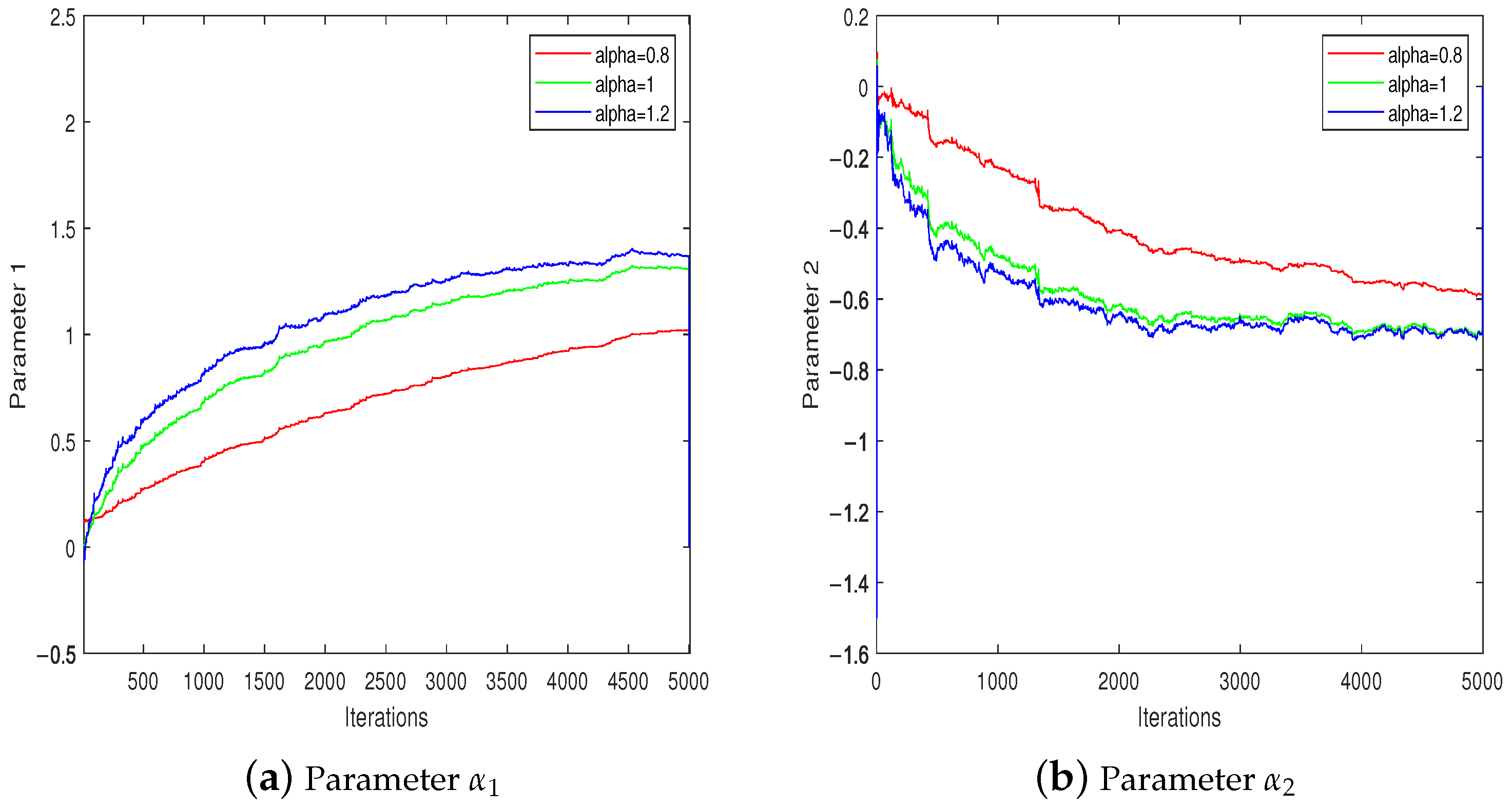
The numerical simulation results are shown in Figure 3, Figure 4 and Figure 5, where the abscissa is the number of iterations. It is shown that the parameters of the AR model could be identified by the algorithms proposed in this article and the figures reflect the effectiveness of the algorithm and that the larger fractional order would bring a faster convergence speed. Meanwhile, the problem of gradient accumulation in the Adagrad method can be relieved by a bigger fractional order as Figure 6 shows.
As Figure 4 and Figure 5 shows, compared with existing algorithms with an integer order gradient—like standard SGD, Adagrad, where μ = 0.1 , and the momentum method, where β t = 0.1 k —the fractional counterpart performs better on convergence but the accuracy is not outstanding for the disturbance of noise. In particular, SGD with momentum and a fractional order has a better result than the other algorithms in terms of convergence speed. That is to say, the fractional gradient SGD method can be applied to other mature algorithms and is likely to perform better than them.

4.2. Example 2

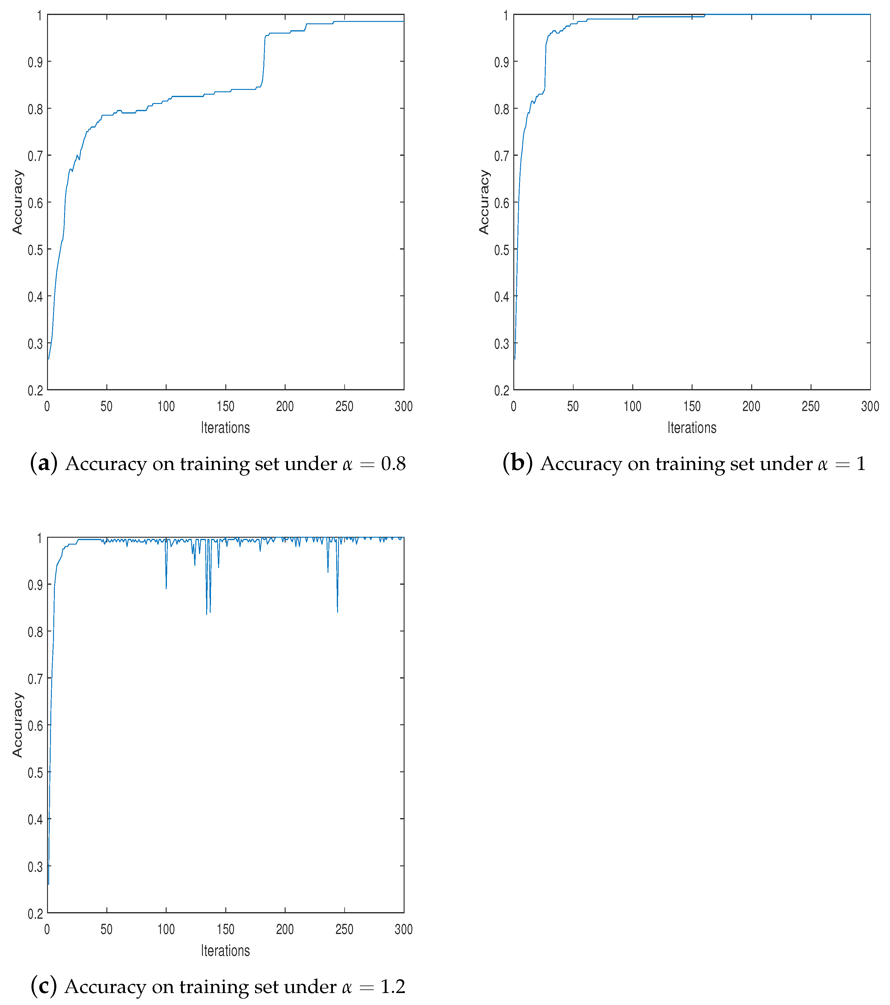
A deep BP neural network with a fractional gradient order is built to test the validity of the proposed algorithm. The data we adopted are from the well-known MNIST dataset, which contains 60,000 handwritten numeral images for training [20]. Each sample of the dataset can be seen as a matrix of 28 28 and the label of each sample is a vector of 10 1 , where the element being 1 is the classification result. The main application of the fractional order gradient is the process of error back propagation, where each layer of the network updates its value of weights from the error between samples and the network weights trained before, and this can be seen as a typical online optimization problem. The batch size set here is 200 and the maximum of number of iterations is 300, which can be checked in Figure 7. The designed network consists of 5 layers which have 64 nodes in a hidden layer and 10 nodes in an output layer. Under the fractional order gradient information, the update of the weight matrix between layers can be described as
W k + 2 = W k + 1 1 Γ ( 2 α ) η n i = 1 n E W k + 1 i ( | W k + 1 i W k i | + δ ) 1 α ,
where E = 1 2 j = 1 l i = 1 n l ( a i j l o i j ) 2 with L 2 regularization, η is the learning rate, and n is the sample size of each batch; set η = 3 k .
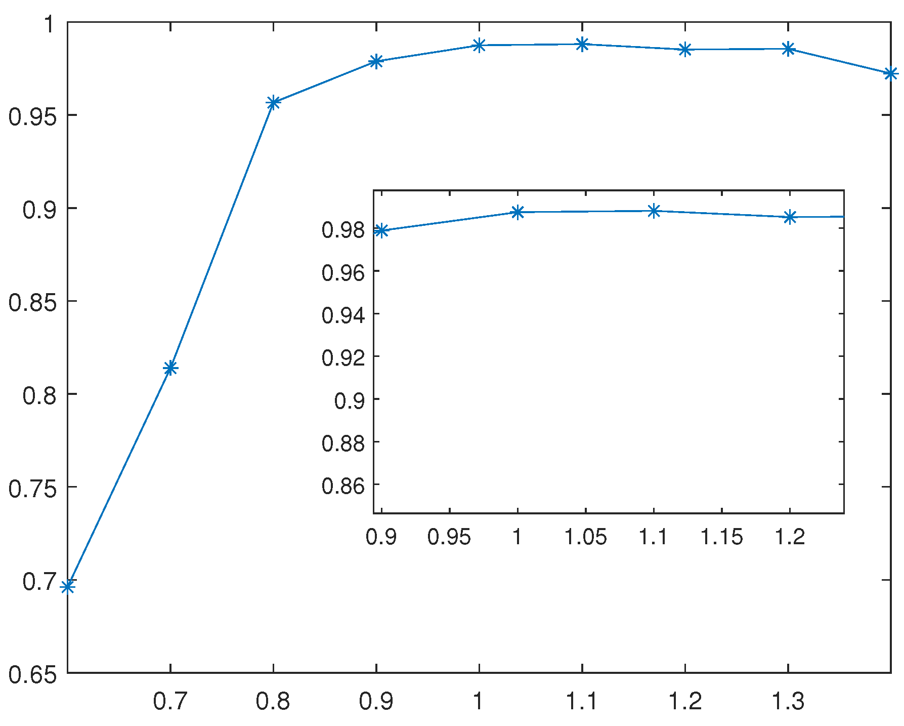
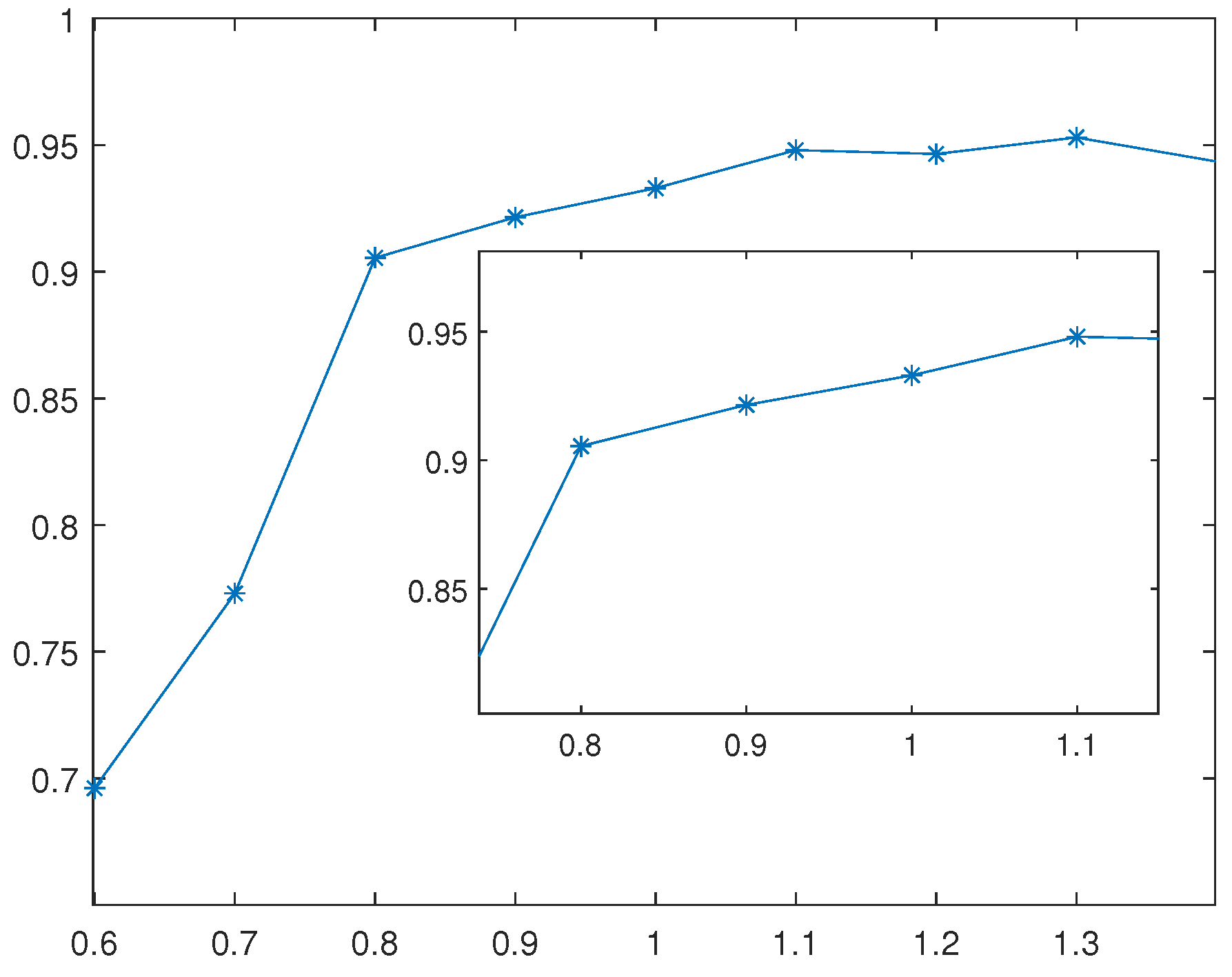
The results are shown in Figure 7, Figure 8 and Figure 9, which reveal the effectiveness of SGD with a fractional order gradient. The degrees of accuracy on the test set are 90.55%, 93.3%, and 94.4%, respectively. The neural network under order 1.2 has a faster convergence speed and higher accuracy on the test set, which is consistent with Theorem 1. Figure 8 shows that order 1.1 has the highest accuracy and other orders larger than 1 would achieve better results than the integer order.

5. Conclusions

In this article, we proposed some improved stochastic fractional order gradient descent algorithms for the online optimization problem; the convergence is given, where the objective functions were assumed to be convex and the gradients were assumed to be bounded. The bounds of the empirical regret functions of the improved SGD with a fractional order were built based on several assumptions, and the proposed algorithm can relieve the gradient exploding problem. Finally, it was shown how the fractional order affects the convergence of the algorithm by way of two practical applications including system identification and classification.
Future work will include studying the variable fractional order stochastic gradient descent algorithm and developing the decentralized version of FOSGD to accommodate larger-scale datasets. While the setting in this article considers an invariable fractional order in a centralized algorithm, which cannot give scope to the advantage of the fractional algorithm, developing the decentralized version with a variable fractional order is in our future agenda.

Author Contributions

Conceptualization, Y.Y.; methodology, Y.Y.; validation, Y.Y. and L.M.; formal analysis, Y.Y.; investigation, Y.Y.; data curation, Y.H.; writing—original draft preparation, Y.Y. and L.M.; writing—review and editing, Y.Y., L.M., Y.H. and F.L.; visualization, Y.H.; funding acquisition, L.M. All authors have read and agreed to the published version of the manuscript.

Funding

This research was funded by the NNSF of China (Grant No. 61973329).

Institutional Review Board Statement

Not applicable.

Informed Consent Statement

Not applicable.

Data Availability Statement

Not applicable.

Acknowledgments

This work is supported by the NNSF of China (Grant No. 61973329) and Project of Beijing Municipal University Teacher Team Construction Support Plan(No. BPHR20220104).

Conflicts of Interest

The authors declare no conflict of interest.

Abbreviations

The following abbreviations are used in this manuscript:
SGDStochastic Gradient Descent
FOGDFractional Order Gradient Descent

References

  1. Jordan, M.I.; Mitchell, T.M. Machine learning: Trends, perspectives, and prospects. Science 2015, 349, 255–260. [Google Scholar] [CrossRef] [PubMed]
  2. Ruder, S. An overview of gradient descent optimization algorithms. arXiv 2016, arXiv:1609.04747. [Google Scholar]
  3. Bottou, L.; Bousquet, O. The tradeoffs of large scale learning. Adv. Neural Inf. Process. Syst. 2007, 20, 1–8. [Google Scholar]
  4. Bottou, L.; Curtis, F.E.; Nocedal, J. Optimization methods for large-scale machine learning. SIAM Rev. 2018, 60, 223–311. [Google Scholar] [CrossRef]
  5. Dean, J.; Corrado, G.; Monga, R.; Chen, K.; Devin, M.; Mao, M.; Ranzato, M.; Senior, A.; Tucker, P.; Yang, K.; et al. Large scale distributed deep networks. Adv. Neural Inf. Process. Syst. 2012, 25, 1223–1231. [Google Scholar]
  6. Zinkevich, M. Online convex programming and generalized infinitesimal gradient ascent. In Proceedings of the 20th International Conference on Machine Learning (ICML-03), Washington, DC, USA, 21–24 August 2003; pp. 928–936. [Google Scholar]
  7. Duchi, J.; Hazan, E.; Singer, Y. Adaptive subgradient methods for online learning and stochastic optimization. J. Mach. Learn. Res. 2011, 12, 2121–2159. [Google Scholar]
  8. Zeiler, M.D. Adadelta: An adaptive learning rate method. arXiv 2012, arXiv:1212.5701. [Google Scholar]
  9. Kingma, D.P.; Ba, J. Adam: A method for stochastic optimization. arXiv 2014, arXiv:1412.6980. [Google Scholar]
  10. Lei, Y.; Hu, T.; Li, G.; Tang, K. Stochastic gradient descent for nonconvex learning without bounded gradient assumptions. IEEE Trans. Neural Netw. Learn. Syst. 2019, 31, 4394–4400. [Google Scholar] [CrossRef]
  11. Wei, Y.; Kang, Y.; Yin, W.; Wang, Y. Generalization of the gradient method with fractional order gradient direction. J. Frankl. Inst. 2020, 357, 2514–2532. [Google Scholar] [CrossRef]
  12. Shin, Y.; Darbon, J.; Karniadakis, G.E. Accelerating gradient descent and Adam via fractional gradients. Neural Netw. 2023, 161, 185–201. [Google Scholar] [CrossRef]
  13. Yin, C.; Chen, Y.; Zhong, S.m. Fractional-order sliding mode based extremum seeking control of a class of nonlinear systems. Automatica 2014, 50, 3173–3181. [Google Scholar] [CrossRef]
  14. Chen, Y.; Gao, Q.; Wei, Y.; Wang, Y. Study on fractional order gradient methods. Appl. Math. Comput. 2017, 314, 310–321. [Google Scholar] [CrossRef]
  15. Chen, Y.; Wei, Y.; Wang, Y.; Chen, Y. Fractional order gradient methods for a general class of convex functions. In Proceedings of the 2018 Annual American Control Conference (ACC), Milwaukee, WI, USA, 27–29 June 2018; IEEE: Manhattan, NY, USA, 2018; pp. 3763–3767. [Google Scholar]
  16. Liu, J.; Zhai, R.; Liu, Y.; Li, W.; Wang, B.; Huang, L. A quasi fractional order gradient descent method with adaptive stepsize and its application in system identification. Appl. Math. Comput. 2021, 393, 125797. [Google Scholar] [CrossRef]
  17. Xue, H.; Shao, Z.; Sun, H. Data classification based on fractional order gradient descent with momentum for RBF neural network. Netw. Comput. Neural Syst. 2020, 31, 166–185. [Google Scholar] [CrossRef]
  18. Mei, J.J.; Dong, Y.; Huang, T.Z. Simultaneous image fusion and denoising by using fractional-order gradient information. J. Comput. Appl. Math. 2019, 351, 212–227. [Google Scholar] [CrossRef]
  19. Zhang, H.; Mo, L. A Novel LMS Algorithm with Double Fractional Order. Circuits Syst. Signal Process. 2023, 42, 1236–1260. [Google Scholar] [CrossRef]
  20. Wang, J.; Wen, Y.; Gou, Y.; Ye, Z.; Chen, H. Fractional-order gradient descent learning of BP neural networks with Caputo derivative. Neural Netw. 2017, 89, 19–30. [Google Scholar] [CrossRef]
  21. Sheng, D.; Wei, Y.; Chen, Y.; Wang, Y. Convolutional neural networks with fractional order gradient method. Neurocomputing 2020, 408, 42–50. [Google Scholar] [CrossRef]
  22. Lacoste-Julien, S.; Schmidt, M.; Bach, F. A simpler approach to obtaining an O (1/t) convergence rate for the projected stochastic subgradient method. arXiv 2012, arXiv:1212.2002. [Google Scholar]
  23. Shalev-Shwartz, S.; Singer, Y.; Srebro, N. Pegasos: Primal estimated sub-gradient solver for svm. In Proceedings of the 24th International Conference on Machine Learning, New York, NY, USA, 20–24 June 2007; pp. 807–814. [Google Scholar]
  24. Chen, X.; Wu, S.Z.; Hong, M. Understanding gradient clipping in private SGD: A geometric perspective. Adv. Neural Inf. Process. Syst. 2020, 33, 13773–13782. [Google Scholar]
  25. Yu, Z.; Sun, G.; Lv, J. A fractional-order momentum optimization approach of deep neural networks. Neural Comput. Appl. 2022, 34, 7091–7111. [Google Scholar] [CrossRef]
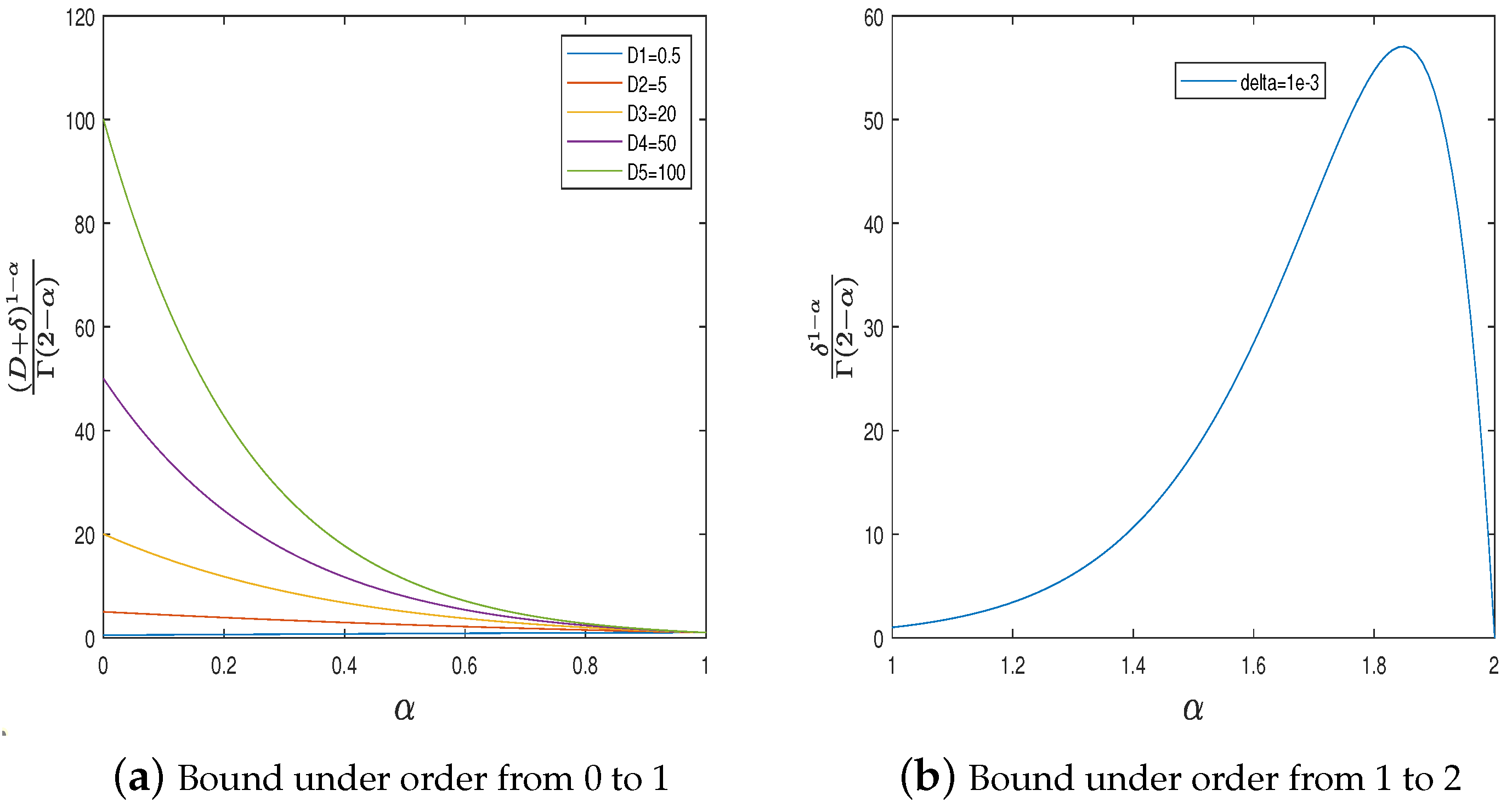
Figure 1. Bound of regret under different orders.
Fractalfract 07 00631 g001
Figure 2. Bound of regret under different orders.
Fractalfract 07 00631 g002
Figure 3. Standard SGD with fractional gradient.
Fractalfract 07 00631 g003
Figure 4. Adagrad method with fractional gradient.
Fractalfract 07 00631 g004
Figure 5. Momentum method with fractional gradient.
Fractalfract 07 00631 g005
Figure 6. Sum of history gradients.
Fractalfract 07 00631 g006
Figure 7. Accuracy on training set under different orders.
Fractalfract 07 00631 g007
Figure 8. Accuracy on train set under orders from 0.6 to 1.4.
Fractalfract 07 00631 g008
Figure 9. Accuracy on test set under orders from 0.6 to 1.4.
Fractalfract 07 00631 g009
Disclaimer/Publisher’s Note: The statements, opinions and data contained in all publications are solely those of the individual author(s) and contributor(s) and not of MDPI and/or the editor(s). MDPI and/or the editor(s) disclaim responsibility for any injury to people or property resulting from any ideas, methods, instructions or products referred to in the content.