Article

Scaling Analysis of Time-Reversal Asymmetries in Fully Developed Turbulence

by
François G. Schmitt
Laboratoire d’Océanologie et de Géosciences, CNRS, University Littoral Cote d’Opale, University Lille, UMR 8187, LOG, F 62930 Wimereux, France
Fractal Fract. 2023, 7(8), 630; https://doi.org/10.3390/fractalfract7080630
Submission received: 27 July 2023 / Revised: 15 August 2023 / Accepted: 16 August 2023 / Published: 18 August 2023

Abstract

:
In fully developed turbulence, there is a flux of energy from large to small scales in the inertial range until the dissipation at small scales. It is associated with irreversibility, i.e., a breaking of the time reversal symmetry. Such turbulent flows are characterized by scaling properties, and we consider here how irreversibility depends on the scale. Indicators of time-reversal symmetry for time series are tested involving triple correlations in a non-symmetric way. These indicators are built so that they are zero for a time-reversal symmetric time series, and a departure from zero is an indicator of irreversibility. We study these indicators applied to two fully developed turbulence time series, from flume tank and wind tunnel databases. It is found that irreversibility occurs in the inertial range and has scaling properties with slopes close to one. A maximum value is found around the injection scale. This confirms that the irreversibility is associated with the turbulent cascade in the inertial range and shows that the irreversibility is maximal at the injection scale, the largest scale of the turbulent cascade.

1. Introduction

Fully developped turbulence is a prototype of complex system possessing many degress of freedoms, huge fluctuations and long-range correlations. In this system, the energy is injected at a large scale, is transferred from large to small scales through the so-called Richardson–Kolmogorov energy cascade, and is dissipated at small scales [1,2]. The scales between the injection and dissipation scales belong to the inertial range, a range of scales of special interest since the early works of the Russian school in turbulence [3,4]. For example, in the inertial range, the Fourier spectral density of the velocity field is scaling with an exponent of −5/3; velocity time series are long-range power-law correlated, and the structure functions (increments of the velocity time series of the form Δ U = U ( x + ) U ( x ) where U is one component fo the velocity field, x is the position and an increment belonging to the inertial range) are intermittent and possess multifractal properties [1,5].
Turbulent flows are also irreversible. Irreversibility in turbulence has been quantitatively studied mainly through the concept of time reversibility: for a time-reversible system, the statistics of the process are invariant by changing the time arrow, i.e., the change of t to t . This has been studied in turbulence by considering the time reversibility of subgrid scales models [6], coherent structures in wall turbulence [7], by following Lagrangian tracers and their dispersion backward and forward [8], by considering the power along Lagrangian trajectories [9,10,11,12,13,14], or by considering their links with singularities, especially using the Eulerian acceleration [15,16]. Time reversibility for nonlinear time series has also been considered in other fields, such as statistical physics [17,18], economy [19,20,21,22] or geosciences [23].
Here, we consider turbulent time series from fully developed turbulence and apply, among the different methods that can be found in the literature, a method involving triple correlations. This has been first proposed by Pomeau [17] in statistical physics, and a similar approach has been later published also in the field of econometrics by Ramsey and Rothamn [19]. Below, in the next section, we first present these methods and propose a straightforward generalization; we further present the two databases of measured fully developed turbulence to which these methods are applied. The next sections present the results and discussions.

2. Material and Methods

2.1. Methods: Tiple Correlations as Indicators of Time-Reversal Asymmetries

Let us consider here one component of the velocity field measured in a wind tunnel or a flume tank: using the usual Taylor hypothesis of frozen turbulence, one-point measurements of the velocity field in time U ( t ) provide statistical information in the Eulerian framework. We consider the zero-mean streamwise velocity u ( t ) = U ( t )     < U > , where < U > is the time average. We assume that this quantity is stationary. The autocorrelation function C u ( τ ) = < u ( t ) u ( t + τ ) > does not depend on t and depends only on τ . By considering a change in time t = t , the new correlation estimated on u * ( t ) = u ( t ) when time moves backward is C u * ( τ ) = < u * ( t ) u * ( t + τ ) > = < u ( t ) u ( t τ ) > . It can be computed by adding 2 t + τ to both terms, providing C u * ( τ ) = < u ( t + τ ) u ( t ) > = C u ( τ ) . This recalls that by construction, the autocorrelation is always invariant by the change in time direction, and that this indicator cannot be used to detect time-reversal asymmetries.
However, triple correlations can be introduced, and with a convenient choice of increments, the time-reversal symmetries can be considered, as proposed some time ago by Pomeau [17,18]. Let us note the triple correlation:
G + ( τ ) = < u ( t ) u ( t + 2 τ ) u ( t + 3 τ ) > .
The same expression applied to the time reversed process u * provides G ( τ ) = < u * ( t ) u * ( t + 2 τ ) u * ( t + 3 τ ) > = < u ( t ) u ( t 2 τ ) u ( t 3 τ ) > . By adding to both terms 2 t + 3 τ , one obtains
G ( τ ) = < u ( t + 3 τ ) u ( t + τ ) u ( t ) > .
The two expressions G + and G are not identical, and their difference P o = G + G can be taken as an indicator of time-reversal symmetry. For a linear or reversible process, this indicator is indentically null.
Another indicator has been proposed in the econometry literature. Ramsey and Rothman [19] have proposed to consider g + ( τ ) = < u 2 ( t ) u ( t + τ ) > . Applying the same procedure as above, we see that g ( τ ) = < u 2 ( t + τ ) u ( t ) > , which is a different expression from g + , and hence, here also the following indicator of time-reversal asymmetry can be proposed:
R R ( τ ) = g + g = < u 2 ( t ) u ( t + τ ) > < u ( t ) u 2 ( t + τ ) > .
This indicator has also been considered later in turbulence [15].
Finally, let us propose here a straightforward generalization. Let us note for s > r the general expression of the triple correlation:
Φ + ( r , s ) = < u ( t ) u ( t + r ) u ( t + s ) > .
By considering the triple correlation Φ ( r , s ) applied on u * , we obtain Φ ( r , s ) = < u ( t ) u ( t r ) u ( t s ) > , which provides, after adding 2 t + s to both terms, Φ ( r , s ) = < u ( t + s ) u ( t + s r ) u ( t ) > . The general indicator can then be written, by taking s = ρ r , ρ 1 , as follows:
Ψ ( r , ρ r ) = < u ( t ) u ( t + r ) u ( t + ρ r ) > < u ( t ) u ( t + ( ρ 1 ) r ) u ( t + ρ r ) > .
We see that ρ = 3 corresponds to Pomeau’s indicator Ψ ( r , 3 r ) = P o ( r ) and ρ = 1 corresponds to the Ramsey–Rothman indicator: R R ( r ) = Ψ ( r , r ) . Below, we first apply these two indicators to fully developed turbulence time series, and then we also apply the general indicator for different values of ρ from 1 to 100.

2.2. Presentation of the Databases

For the test of the above-mentioned indicators, two fully developed turbulence databases were chosen. The first one is recorded using the IFREMER wave and current flume tank (Boulogne-sur-mer, France). The flow turbulent velocity is measured using a Laser Doppler Velocimeter during three hours with an irregular sampling rate that goes up to 900 Hz. The working section of the system is 4 m in width by 2 m in depth and 18 m in length. The streamwise flow velocity has a mean value of < U > = 0.8 m/s, a turbulence intensity (ratio of the standard deviation of the streamwise component to its mean value) of 20%, a dissipation rate value of ϵ = 1.79 × 10 2 m 2 s 3 and a Taylor-based Reynolds number of R λ = 487 [24]. The data are freely available through the SEANOE depository [25]. We consider here the data resampled at a fixed resolution of 100 Hz and a number of datapoints of N = 2 19 .
The second database is a wind tunnel database of turbulence velocity time series obtained from an experimental homogeneous and nearly isotropic turbulent flow from Johns Hopkins University [26]. We consider here time series recorded at downstream x / M = 20, where M is the mesh size. The sampling frequency is f 0 = 40 kHz, the mean velocity < U > = 12 m/s, the rms velocity is 1.85 m/s and the Taylor-based Reynolds number R λ = 720 . The total duration analyzed is 30 s, and the number of data points per channel is 1.2 × 10 6 . Since there are 120 realizations and four channels, the total number of data points at this location is 5.76 × 10 8 . The scaling properties of this time series have already been studied using different methods and found to be visible over two decades [27,28].
As a first analysis of both these datasets, Fourier spectral analysis is shown in the log–log plot in Figure 1, where f 0 in both cases is the sampling frequency (100 Hz for the flume tank and 40 kHz for the wind tunnel databases). A dotted line of slope 5 / 3 is shown for reference: in both cases, a scaling property is visible over more than two decades.
Let us introduce here the classical structure functions of order 2: < Δ u 2 > where Δ u = u ( t + τ ) u ( t ) (structure functions in time and we are still using Taylor’s frozen turbulence hypothesis). Direct calculation shows that 1 C u ( τ ) = < Δ u 2 > / ( 2 σ u 2 ) . In the framework of intermittent multifractal turbulence, < Δ u 2 > τ α with α 2 / 3 . Hence, the plot of 1 C u ( τ ) shows, in real space, the scaling properties of the structure functions and also their scaling range. This is displayed in Figure 2 for both databases: the scaling range is still clearly visible, with an amplitude which is slightly smaller in the real space compared to the spectral space (this has been studied and explained in other works [5]). The scale range from r = 10 r 0 to 400 r 0 (where r 0 is the time resolution of the measurements) is here the visible scaling inertial range, which is used further for triple correlation analyses.

3. Results: Triple Correlation Analyses and Time Reversal Symmetries

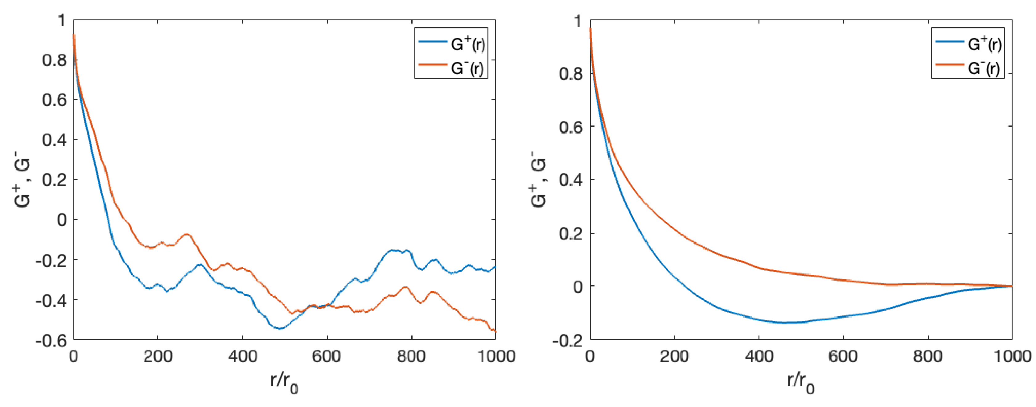
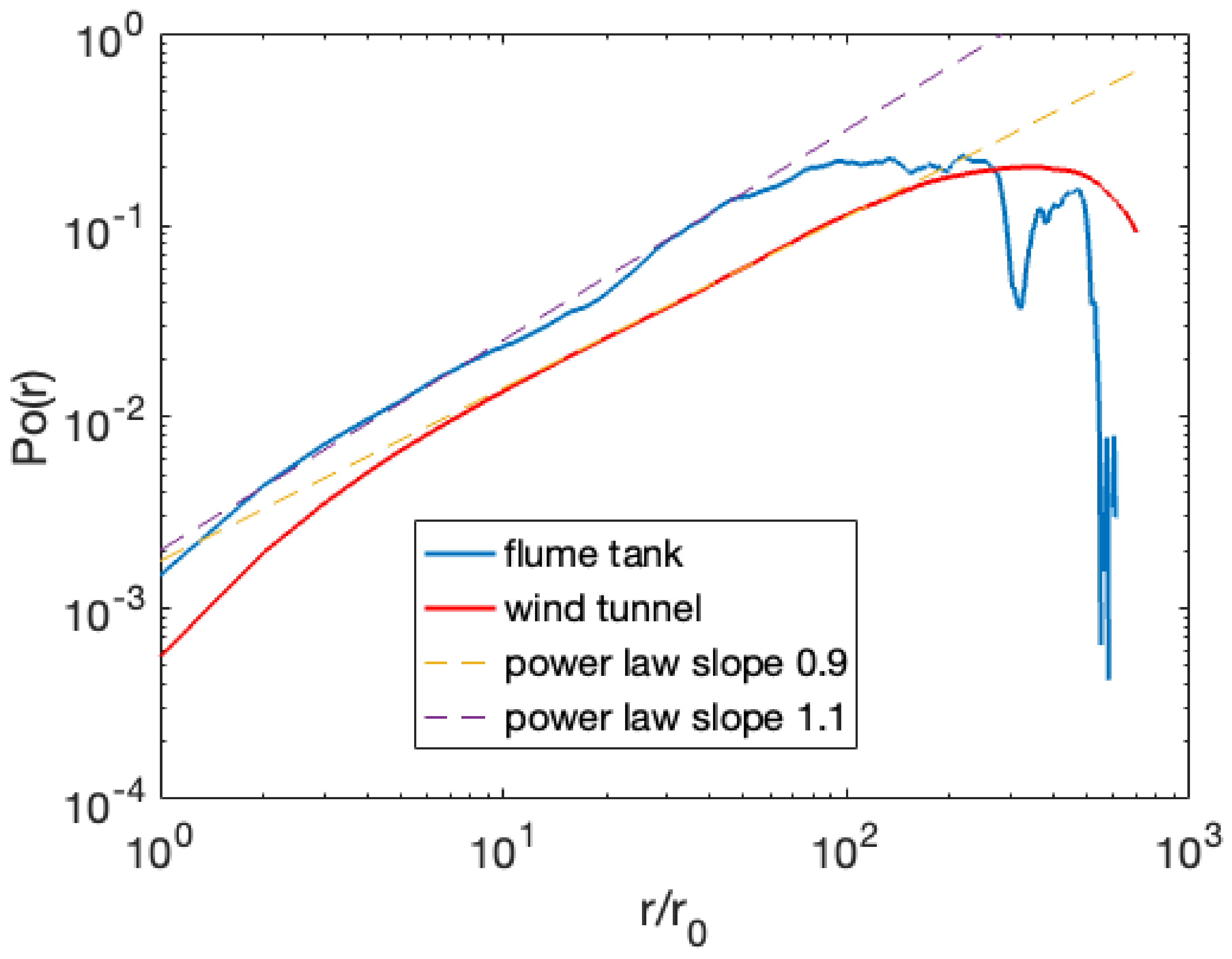
We first display the two indicators G + and G corresponding to Equations (1) and (2), normalized by the third-order moment < u 3 > , in Figure 3a,b. It is visible that these two functions do not coincide in both cases, indicating a time-reversal asymmetry. They join at a large scale. Since there are more data for the wind tunnel case, the curves are smoother for this database. In order to emphasize the scaling properties, their difference (still with the normalization of the third-order moment) P o = G + G is represented in the log–log plot in Figure 4. It is seen in both cases that a scaling behaviour is found with slopes of approximately 0.9 for the wind tunnel and 1.1 for the flume tank databases. The scaling ranges seem to be slightly different from the structure functions. Furthermore, in both cases, a maximum value is reached after which the indicator decreases. This maximum value is approximately the same as the upper bound of the scaling range.
We next consider the indicators corresponding to the Ramsey–Rothman indicator g + and g and the indicator R R given by Equation (3). This is shown in Figure 5a,b and Figure 6. First, as for the previous indicator, the two curves are clearly different, indicating time-reversal asymmetry. They join at a large scale whose value is larger than that for the previous indicator. Their difference, shown in Figure 6, is also scaling with scaling exponents that seem to be the same as those for P o . In both plots, there is a maximum value and a decrease in the indicator before reaching the value of zero.
After these first results, we can consider the generalized indicator Ψ ( r , ρ r ) given by Equation (5). We perform this by representing Ψ ( r , ρ r ) vs. r for different values of ρ from 1 to 100. This is illustrated in Figure 7a,b for both databases displayed for four different values of s: s = 3 , 5, 10 and 20. A common feature is found for both curves: their scaling slope is the same (the curves are parallel); there is a maximum value after which the curve is decreasing, and this maximal value is found for smaller values of r as s increases; finally, the maximum value of the indicator is increasing when s is increasing.
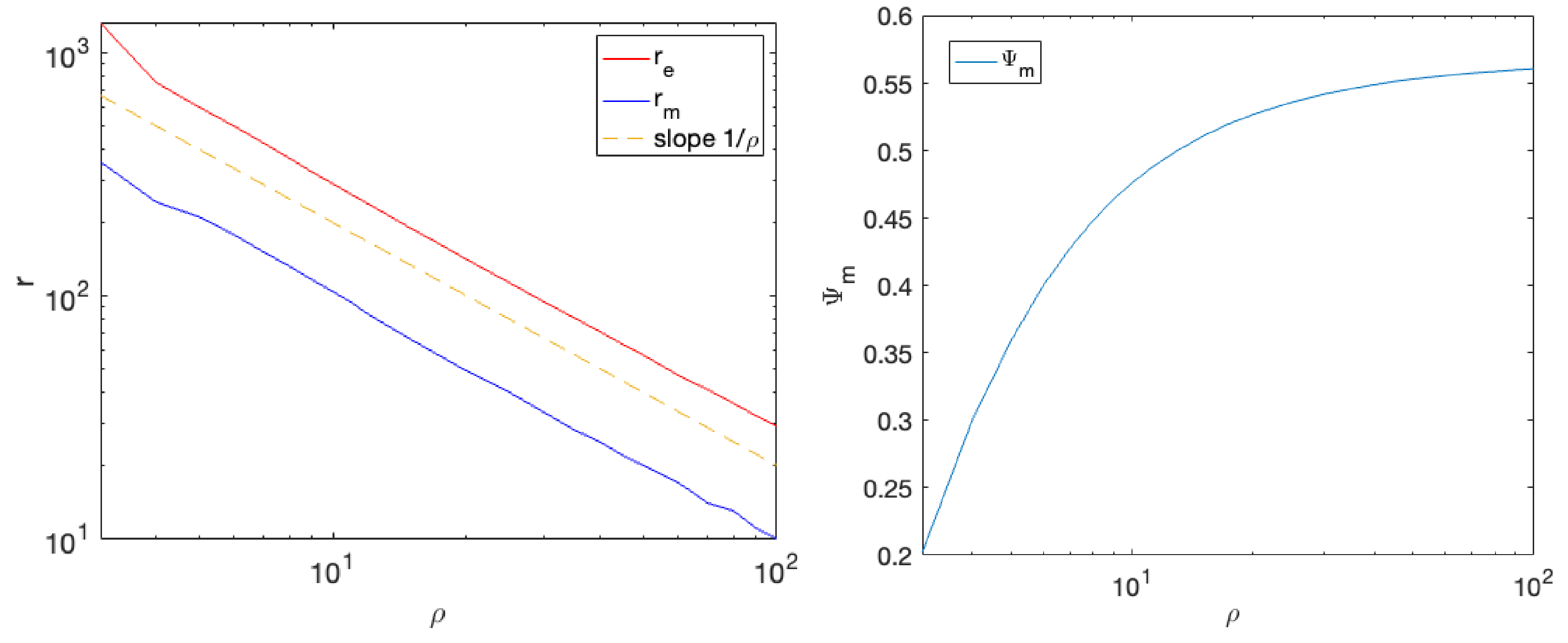
In each case, we record the maximum value Ψ max = max r { Ψ ( r , ρ r ) } , the location of this maximal value r m such that Ψ ( r m , ρ r m ) = Ψ max and also the location for which the indicator is first reaching 0: Ψ ( r e , ρ r e ) = 0 . These variables are shown in Figure 8a,b (only for the wind tunnel database, but the results are the same for the flume tank database). It is found that both positions r m and r e are inversely proportional to ρ . The maximum value Ψ max is increasing with ρ and reaching a plateau for large values of ρ .

4. Discussion and Conclusions

We considered here two databases of fully developed turbulence: flume tank and wind tunnel databases. In each case, there are scaling properties of different turbulent quantities, such as the power spectrum with slope 5 / 3 and structure functions of Order 2 with slope 2 / 3 over a given range of scales corresponding to the inertial range (Figure 1 and Figure 2). Using these databases, several indicators based on triple correlation functions have been estimated: Figure 4 and Figure 6 show two first indicators proposed, respectively, by Pomeau [17] and by Ramsey and Rothman in the finance framework [19] (let us note here that the R R indicator from Equation (3) has already been estimated in turbulence by Josserand et al. [15] in a work devoted to the energy cascade in turbulence). The fact that the forward and backward terms are not equal is a clear indication of time-symmetry breaking. Figure 4 and Figure 6 show that these indicators have some scaling properties, with different slopes for the flume tank and wind tunnel databases. These slopes are found to be close to one in each case. These indicators of time-reversal asymmetry are scaling in the inertial range: they increase with the scale r and they decrease at a large scale which is close to the outer scale of the inertial range. The slight difference in scaling slopes found here could be explained by differences in Reynolds numbers. The slope close to one of these third-order moments could also be related to the energy balance equation in the analogy with the exponent one found for the third-order structure function in the inertial range.
We also introduced a more general indicator, still based on triple correlations Ψ ( r , ρ r ) , and by changing the value of ρ from 3 to 100, we found a similar behaviour with a scaling range, smaller for larger values of ρ , a maximum value of the indicator, and a large scale which is decreasing with the increasing values of ρ : in fact, the product ρ × r m is constant, and what is illustrated here is the fact that when increasing ρ , the values of r for which there is irreversibility are decreasing because the product must stay inside the inertial range.
In the Navier–Stokes equations, the only term which is not time reversible is the viscous dissipation term. This is one fundamental source of irreversibility, but for fully developed turbulence, the dissipation occurs at small scales, whereas we found here that the irreversibility, as shown by the indicators of time-reversal asymmetry, is larger in the inertial range than at viscous scales. The irreversibility is even more visible around the outer scale of the inertial range. This result is compatible with those of previous works: it is often mentioned that one of Kolmogorov’s 1941 results [29], the famous ‘−4/5’ law, i.e., < U ( x + ) U ( x ) 3 > = 4 5 ϵ in the inertial range, is indicative of irreversibility: a non-zero third moment means that time reversibility is broken [30], and since this law is valid in the inertial range, our quantitative and experimental result is in agreement with this theoretical relation. Using other methods, previous works also found that the irreversibility of turbulent flows is occuring in the inertial range through the turbulent cascade [9,11,31].
An interesting discussion around this was proposed in a recent paper [32] that recalled that the source of irreversibility in the Navier–Stokes equations is viscosity, so that, e.g., Euler equations (Navier–Stokes without the viscous term) are reversible. However, even from the Euler equations, there are nonlinear terms that generate what can be called “statistical irreversibility“ corresponding to the chaotic properties of the flow at larger scales. This has been also shortly discussed by Davidson in his monograph [33]: the arrow of time, i.e., irreversibility was seen as coming from the nonlinear terms of Navier–Stokes equations, and from these terms, statistically, the behaviour is chaotic and irreversible. The indicators which are tested here provide a quantitative confirmation of these qualitative comments and show also that this statistical irreversibility is dominant in the inertial range, displaying the most visible effect around the injection scale of the turbulence. Another interpretation may be to consider that at the outer scale of the turbulence, boundary conditions contribute to violate the symmetries of the Navier–Stokes equations, contributing to irreversibility, and that symmetries are progressively restored statistically during the cascade process until reaching the smaller scales.
As perspectives of this work, we can mention the objective of obtaining such results from the Navier–Sokes equations. Indeed, the results presented here are fully experiment-based and there are, to our knowledge, no theoretical attempts able to explain these results from the basic equations; a possible starting point could be the energy balance equation, as mentioned above. Finally, we may also emphasize the fact that there are many time series from natural sciences that seem (from visual inspection) to have time-reversal asymmetries. The indicators here are interesting and easy-to-apply candidates to provide quantitative assessments of irreversibilities in recorded time series.

Funding

This research received no external funding.

Data Availability Statement

The two databases that are used here are freely available online.

Acknowledgments

Comments and suggestions by reviewers are acknowledged.

Conflicts of Interest

The author declares no conflict of interest.

References

  1. Frisch, U. Turbulence: The Legacy of A.N. Kolmogorov; Cambridge University Press: Cambridge, UK, 1995. [Google Scholar]
  2. Pope, S.B. Turbulent Flows; Cambridge University Press: Cambridge, UK, 2000. [Google Scholar]
  3. Kolmogorov, A.N. Local structure of turbulence in an incompressible fluid at very high Reynolds numbers. Dokl. Akad. Nauk SSSR 1941, 30, 299–303. [Google Scholar] [CrossRef]
  4. Obukhov, A.M. Spectral energy distribution in a turbulent flow. Dokl. Akad. Nauk SSSR 1941, 32, 22–24. [Google Scholar]
  5. Schmitt, F.G.; Huang, Y. Stochastic Analysis of Scaling Time Series: From Turbulence Theory to Applications; Cambridge University Press: Cambridge, UK, 2016. [Google Scholar]
  6. Fang, L.; Bos, W.J.T.; Shao, L.; Bertoglio, J.-P. Time reversibility of Navier-Stokes turbulence and its implication for subgrid scale models. J. Turbul. 2012, 13, 1–14. [Google Scholar] [CrossRef]
  7. Iacobello, G.; Chowdhuri, S.; Ridolfi, L.; Rondoni, L.; Scarsoglio, S. Coherent structures at the origin of time irreversibility in wall turbulence. Comm. Phys. 2023, 6, 91. [Google Scholar]
  8. Jucha, J.; Xu, H.; Pumir, A.; Bodenschatz, E. Time-reversal-symmetry breaking in turbulence. Phys. Rev. Lett. 2014, 113, 054501. [Google Scholar] [CrossRef]
  9. Xu, H.; Pumir, A.; Falkovich, G.; Bodenschatz, E.; Shats, M.; Xia, H.; Francois, N.; Boffetta, G. Flight-crash events in turbulence. Proc. Natl. Acad. Sci. USA 2014, 111, 7558–7563. [Google Scholar] [CrossRef]
  10. Xu, H.; Pumir, A.; Bodenschatz, E. Lagrangian view of time irreversibility of fluid turbulence. Sci. China-Phys. Mech. Astron. 2016, 59, 614702. [Google Scholar] [CrossRef]
  11. Pumir, A.; Xu, H.; Bodenschatz, E.; Grauer, R. Single-particle motion and vortex stretching in three-dimensional turbulent flows. Phys. Rev. Lett. 2016, 116, 124502. [Google Scholar] [CrossRef]
  12. Vencini, M.; Biferale, L.; Boffetta, G.; De Pietro, M. Time irreversibility and multifractality of power along single particle trajectories in turbulence. Phys. Rev. Fluids 2017, 2, 104604. [Google Scholar] [CrossRef]
  13. Bhatnagar, A.; Gupta, A.; Mitra, D.; Pandit, R. Heavy inertial particles in turbulent flows gain energy slowly but lose it rapidly. Phys. Rev. E 2018, 97, 033102. [Google Scholar] [CrossRef]
  14. Picardo, J.R.; Bhatnagar, A.; Ray, S.S. Lagrangian irreversibility and Eulerian dissipation in fully developed turbulence. Phys. Rev. Fluids 2020, 5, 042601. [Google Scholar] [CrossRef]
  15. Josserand, C.; Le Berre, M.; Lehner, T.; Pomeau, Y. Turbulence: Does energy cascade exist? J. Stat. Phys. 2017, 167, 596–625. [Google Scholar] [CrossRef]
  16. Le Berre, M.; Pomeau, Y. Singularities in turbulent flows: How to observe them? Phys. D 2023, 443, 133563. [Google Scholar] [CrossRef]
  17. Pomeau, Y. Symétrie des fluctuations dans le renversement du temps. J. Phys. 1982, 43, 859–867. [Google Scholar] [CrossRef]
  18. Pomeau, Y. Time in science: Reversibility vs. irreversibility. Lect. Notes Phys. 2004, 644, 425–436. [Google Scholar]
  19. Ramsey, J.B.; Rothman, P. Time irreversibility and business cycle asymmetry. J. Money Credit Bank. 1996, 28, 1–21. [Google Scholar] [CrossRef]
  20. Cheng, Q. On time-reversibility of linear processes. Biometrika 1999, 86, 483–486. [Google Scholar] [CrossRef]
  21. Chen, Y.T.; Chou, R.Y.; Kuan, C.M. Testing time reversibility without moment restrictions. J. Econom. 2000, 95, 199–218. [Google Scholar] [CrossRef]
  22. Psaradakis, Z. Assessing time-reversibility under minimal assumptions. J. Time Ser. Anal. 2008, 29, 881–905. [Google Scholar] [CrossRef]
  23. Telesca, L.; Flores-Marquez, E.L.; Ramirez-Rojas, A. Time-reversibility in seismic sequences: Application to the seismicity of Mexican subduction zone. Physica A 2018, 492, 1373–1381. [Google Scholar] [CrossRef]
  24. Duran Medina, O.; Schmitt, F.G.; Calif, R.; Germain, G.; Gaurier, B. Turbulence analysis and multiscale correlations between synchronized flow velocity and marine turbine power production. Renew. Energy 2017, 112, 314–327. [Google Scholar] [CrossRef]
  25. Gaurier, B.; Germain, G.; Facq, J.-V.; Bacchetti, T.; Duran-Medina, O. Experimental measurements of a synchronized flow velocity and a marine current turbine power production. SEANOE 2018. [Google Scholar] [CrossRef]
  26. Kang, H.; Chester, S.; Meneveau, C. Decaying turbulence in an active-grid-generated flow and comparisons with large-eddy simulation. J. Fluid Mech. 2003, 480, 129–160. [Google Scholar] [CrossRef]
  27. Huang, Y.X.; Schmitt, F.G.; Lu, Z.M.; Liu, Y.L. An amplitude-frequency study of turbulent scaling intermittency using Empirical Mode Decomposition and Hibert Spectral Analysis. Europhys. Lett. 2008, 84, 40010. [Google Scholar] [CrossRef]
  28. Huang, Y.X.; Schmitt, F.G.; Lu, Z.M.; Liu, Y.L. Autocorrelation function of velocity increments time series in fully developed turbulence. Europhys. Lett. 2009, 86, 40010. [Google Scholar] [CrossRef]
  29. Kolmogorov, A.N. Dissipation of energy in locally isotropic turbulence. Dokl. Akad. Nauk SSSR 1941, 32, 19–21. [Google Scholar]
  30. Falkovich, G. Symmetries of the turbulent state. J. Phys. A Math. Theor. 2009, 42, 123001. [Google Scholar] [CrossRef]
  31. Verma, M.K. Asymmetric energy transfers in driven nonequilibrium systems and arrow of time. Eur. Phys. J. B 2019, 92, 190. [Google Scholar] [CrossRef]
  32. Vela-Martin, A.; Jimenez, J. Entropy, irreversibility and cascades in the inertial range of isotropic turbulence. J. Fluid Mech. 2021, 915, A36. [Google Scholar] [CrossRef]
  33. Davidson, P.A. Turbulence, an Introduction for Scientists and Engineers; Oxford University Press: Oxford, UK, 2015. [Google Scholar]
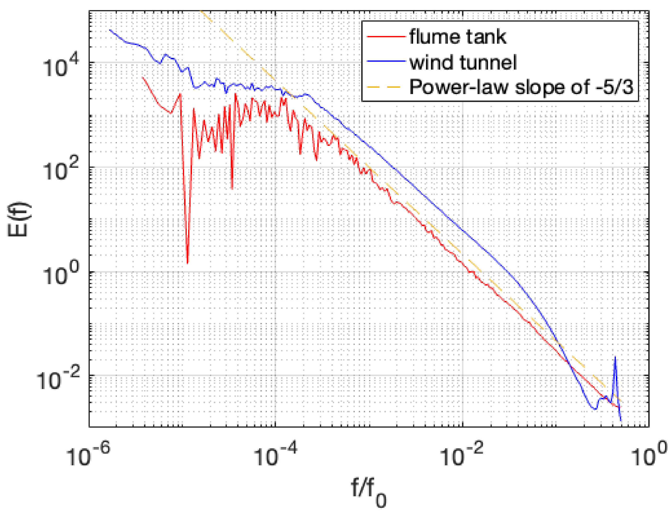
Figure 1. Fourier of the two series showing their scaling properties where f 0 is the sampling frequency. A dotted line with slope 5 / 3 is shown for reference.
Fractalfract 07 00630 g001
Figure 2. Plot of the second-order structure function, showing the scaling range in the real space. A dotted line of slope 2 / 3 is shown for reference.
Fractalfract 07 00630 g002
Figure 3. Representation of the two functions G + and G for both databases (left: the flume tank and right: the wind tunnel). In both cases, it is visible that these functions are clearly different and join only at a large scale.
Fractalfract 07 00630 g003
Figure 4. Superpositions of log–log plots of the indicator P o estimated for both databases.
Fractalfract 07 00630 g004
Figure 5. Representation of the two functions g + and g for both databases (left: the flume tank and right: the wind tunnel). As in Figure 3, in both cases, it is visible that these functions are clearly different and join only at a large scale. The scale at which they join is larger than for the previous indicator.
Fractalfract 07 00630 g005
Figure 6. Superpositions of log–log plots of the indicator R R estimated for both databases.
Fractalfract 07 00630 g006
Figure 7. Representation of the indicator Ψ ( r , ρ r ) for both databases and for several values of ρ ( ρ = 3 , 5, 10 and 20) (left: the flume tank and right: the wind tunnel). The curves are parallel; hence, they are with the same scaling exponents but with different maxima and also different maxima locations.
Fractalfract 07 00630 g007
Figure 8. Left: the two characteristic scales r m and r e corresponding, respectively, to the maximum value of the indicator and to its first zero value, represented in contrast to ρ for different values from ρ = 3 to 100. A dotted line proportional to ρ 1 is shown for comparison. Right: the maximum value of the indicator Ψ max versus ρ in log-linear plot. An increase is found until a plateau reached for larger values of ρ . These plots are obtained from the wind tunnel database.
Fractalfract 07 00630 g008
Disclaimer/Publisher’s Note: The statements, opinions and data contained in all publications are solely those of the individual author(s) and contributor(s) and not of MDPI and/or the editor(s). MDPI and/or the editor(s) disclaim responsibility for any injury to people or property resulting from any ideas, methods, instructions or products referred to in the content.