Article

Investigation of Egyptian Banks’ Competition through a Riesz–Caputo Fractional Model

1
Physics and Engineering Mathematics Department, Faculty of Engineering, Ain Shams University, Cairo 11517, Egypt
2
Physics and Engineering Mathematics Department, Higher Institute of Engineering, El-Shorouk Academy, El-Shorouk City 11837, Egypt
*
Authors to whom correspondence should be addressed.
Fractal Fract. 2023, 7(6), 473; https://doi.org/10.3390/fractalfract7060473
Submission received: 21 May 2023 / Revised: 11 June 2023 / Accepted: 12 June 2023 / Published: 14 June 2023
(This article belongs to the Section General Mathematics, Analysis)

Abstract

:
In this paper, a four-dimensional competition model, driven by the Riesz–Caputo operator, is established. Then, the presented model’s uniqueness, existence, and stability are discussed. After that, the model is applied to describe the profit competition between Egyptian banks. Using the Hamiltonian definition of optimal control, we set a control strategy for banks’ profits during crises as a pre-step measure to counteract their negative impact. Finally, the model is solved numerically using an extended Adams–Bashford scheme. The valid data between the end of 2016 and 2020 are used for numerical simulations, while the data between the end of 2021 and 2022 are used for prediction measurements. From the results, it can be seen that the COVID-19 crisis resulted in a sudden decrease in banks’ profits during 2020, and if there were a control system enabled, it could have compensated for this decrease.

1. Introduction

Mathematical modeling is regarded as an effective apparatus to recognize the future dynamics and other related properties of real-life phenomena in both science and engineering [1,2,3,4,5,6,7,8,9,10,11,12,13,14,15,16,17,18,19,20,21]. This key modeling process can set out policies and recommendations for the advancement of society and humans. Mathematical models are not just useful for solving issues in science and engineering; they are also becoming more popular in disciplines connected to economics, such as banking and finance, which are crucial for economic development. The banking sector and competition between banks are usually modeled by means of a mathematical competition model, which is mainly a system of integer-order ordinary differential equations (ODEs) [3,4].
In recent studies, fractional differential equations have attracted a lot of interest because they ultimately converge to the integer-order system response. This is due to the reduction in formulation employing integer-order derivatives. Furthermore, they have the advantage of strong adaptability in modeling and pointing out the characteristics of several dynamical processes [5,6,7,8,9,10,11,12,13,14,15]. For example, the Fisher equations are transformed into a fractional order form and then solved numerically using the collocation method in [6], while an expression for a fractional time delay model with a variable order is examined in [7]. The authors of [8] applied an innovative numerical solution to a fractional advection equation utilized in their study. In [9], brand-new methods for figuring out fractional-order models that crop up in science and engineering were considered. The authors of [10] developed a time-fractional coupled mkdv equation and solved it using the homotopy method. To investigate the dynamics of the spread of coronavirus (COVID-19), the authors of [11] developed a mathematical model using fractional derivatives and then solved it numerically using the appropriate numerical scheme. The authors of [12] modeled COVID-19 spread by considering spatial effects, quarantine, and isolation principles in their fractional order modeling equations. In [13], a fractional-order system of ODEs was examined with optimal control analysis. A fractional nonlinear oscillator model with coordinate-dependent mass is examined in [14] and solved numerically using the fractional complex transformation. The authors of [15] defined a new fractional operator and applied it to heat diffusion equations. In the case of a bank competition model, many researchers have started working on extending the integer-order model into a fractional-order one to provide a higher accuracy of fitting [16,17,18,19]. In [20,21], it was demonstrated why the fractional-order method is regarded as superior to the integer-order method by providing significantly more options for the best setting of data fitting.
The Egyptian banking system is mainly composed of 33 banks, as stated by the central bank of Egypt (CBE), which can be divided into four categories: public banks, private and Arabic banks, foreign banks, and investment collaboration banks [22]. All of these banks are subject to the instructions announced by CBE. The CBE serves as both the country’s central bank and the national monetary authority. Its main role, like all other central banks, is to regulate both local and foreign banks. It is also responsible for formulating and implementing Egypt’s banking policy, issuing banknotes and coins, maintaining gold and foreign exchange reserves for the country, supervising national currency transaction, and managing Egypt’s private and public loans. There may be competition between the four previously mentioned bank categories because there is no discernible difference in their business areas, and this will be our focus in this study.
This work provides a four-dimensional fractional-order competition model driven by the Riesz–Caputo operator. The model’s uniqueness, existence, and stability are fully examined. Then, more novelty is added by formulating a reinvestment-control function for the proposed model that maximizes the banks’ profits as a pre-step measure to counteract the negative impact of different crises. The developed model is applied to the categories of Egyptian banks that were previously mentioned and solved numerically using a modified Adams–Bashford scheme.
This article is presented in section-wise form as follows: Section 2 mentions the used fractional operator’s mathematical definition. Section 3 introduces the proposed fractional competition model and investigates its uniqueness, existence, stability, and equilibrium. The optimal control process is fully illustrated in Section 4. The numerical procedure using an extended Adams–Bashford scheme to solve our model is obtained in Section 5. In Section 6 and Section 7, respectively, the simulation results and combined conclusions are discussed.

2. Preliminaries

To proceed to our mathematical model of the banks’ competition, we need the following basic definitions and lemmas of fractional calculus.
Definition 1.
Let  ϱ > 0 ,   ρ ( x ) C [ m , n ] . The left and right Riemann–Liouville integral operators of order  ϱ , respectively, are defined as [23]:
l x ϱ m ρ x = 1 Γ ϱ m x x υ ϱ 1 ρ υ d υ ,
and
l n ϱ x ρ x = 1 Γ ϱ x n υ x ϱ 1 ρ υ d υ ,
where  Γ ( ϱ )  is the classical Euler Gamma function.
Definition 2.
Let  ϱ > 0 ,   ρ ( x ) C [ m , n ] . The Riesz integral operator of order  ϱ  is defined as follows [24]:
l n ϱ m R ρ x = 1 2 Γ ϱ m n x υ ϱ 1 ρ υ d υ ,
It is can be seen that the left and right Riemann–Liouville integral operators are related to the Riesz integral operator via the following formula:
l n ϱ m R ρ x = 1 2 ( l x ϱ m ρ ( x ) + l n ϱ x ρ ( x ) ) , ϱ > 0
Definition 3.
Let  ϱ ( r 1 , r ] ,   n N . The left and right Riemann–Liouville fractional derivatives of order  ϱ  take the form [23]:
D x ϱ m ρ x = 1 Γ n ϱ d d x r m x x υ r ϱ 1 ρ υ d υ ,
and
D n ϱ x ρ x = 1 Γ n ϱ d d x r x n v x r ϱ 1 ρ υ d υ
Definition 4.
Let  ϱ ( r 1 , r ] ,   n N . The left and right Caputo fractional derivatives of order  ϱ  take the form [23]:
D x ϱ m c ρ x = 1 Γ n ϱ m x x υ r ϱ 1 d d v r ρ υ d υ ,
and
D n ϱ x c ρ x = 1 Γ n ϱ x n v x r ϱ 1 d d v r ρ υ d υ ,
where  ρ ( x ) C r [ m , n ] .
In many papers, authors prefer to use the Caputo definition of differentiation of fractional order because its properties are similar to the classical definition of ordinary differentiation. For example, if we try to substitute the function ρ ( x ) with a constant, we find that its differentiation is zero, but in the Riemann–Liouville definition, it is not zero. In recent years, many other definitions of fractional differentiation have been produced by several authors, such as Caputo-Fabrizio and Atangana [16,18,23,24,25,26]. One of the most important definitions of the differentiation of fractional order is the Riesz definition, which is related to both the Riemann–Liouville and Caputo definitions and gives important results in the field of calculus of variation.
Definition 5.
Let  ϱ ( r 1 , r ] ,   n N . The Riesz and Riesz–Caputo fractional derivatives of order  ϱ  can be written in the form [24]:
D n ϱ m R ρ x = 1 Γ n ϱ d d x r m n x v r ϱ 1 ρ υ d υ
and
D n ϱ m R c ρ x = 1 Γ n ϱ x n x v r ϱ 1 d d v r ρ υ d υ
where  ρ ( x ) C r [ m , n ] . Using the previous definitions, we find that:
D n ϱ m R ρ x = 1 2 D x ϱ m ρ x 1 n D n ϱ x ρ x ,
and
D n ϱ m R c ρ x = 1 2 D x ϱ m c ρ x 1 n D n ϱ x c ρ x
Lemma 1.
Let the function  ρ ( x )  have a continuous Riesz–Caputo derivative of order  ϱ ,   0 < ϱ < 1 ,  in the interval  [ m , n ]  and we wish to minimize the functional:
m n A ( x , ρ ( x ) , D n ϱ m R c ρ ( x ) ) d x ,
with the boundary conditions  ρ ( m ) = ρ 0  and  ρ ( n ) = ρ 1 , then  ρ ( x )  is necessary to satisfy the Euler–Lagrange equation:
A ρ D n ϱ m R A D n ϱ m R c ρ x = 0 .
We observe that for ϱ = 1 , Equation (13) is similar to the classical Euler–Lagrange equation in calculus of variation which takes different forms if we use Riemann–Liouville or Caputo fractional derivatives. More details can be found in [23].
Lemma 2.
The left and right Riemann-Liouville and Riesz integral operators satisfy the following formulas [24]:
l t ϱ 0 D t ϱ 0 c ρ ( t ) = ρ ( t ) r = 0 n 1 ρ ( r ) ( 0 ) ( t 0 ) r r ! ,
l T ϱ t D T ϱ t c ρ ( t ) = ( 1 ) n ( ρ ( t ) r = 0 n 1 ( 1 ) r ρ ( r ) ( T ) ( T t ) r r ! ) ,
l T ϱ 0 D T ϱ 0 R c ρ ( t ) = 1 2 ( l t ϱ 0 D t ϱ 0 c + l T ϱ t D t ϱ 0 c ) ρ ( t ) + ( 1 ) n 1 2 ( l t ϱ 0 D T ϱ t c + l T ϱ t D T ϱ t c ) ρ ( t )
= 1 2 ( l t ϱ 0 D t ϱ 0 c + ( 1 ) n l T ϱ t D T ϱ t c ) ρ ( t ) ,
where  ρ ( t ) C n [ 0 , T ] .
If 0 < ϱ < 1 and ρ ( t ) C [ 0 , T ] , we find that:
l T ϱ 0 D T ϱ 0 R c ρ ( t ) = ρ ( t ) 1 2 ( ρ ( 0 ) + ρ ( T ) ) .
From the previously illustrated preliminaries, we used the Riesz–Caputo model to derive the proposed competition model due to the fact that:
-
It is more general than the Caputo fractional derivative and can be easily transformed into the Caputo fractional derivative definition.
-
It sets a generalization to the Euler–Lagrange equation, as in (13), which is more general than the classical Euler–Lagrange equation.
-
It transforms into a Riesz fractional derivative in the same interval, while the left Caputo derivative transforms into the right Caputo and vice versa, and this can be easily proved using fractional integration by parts rules in [24].

3. Governing Model

Many authors used the Lotka–Volterra model in the commercial field to perform a comparison between the profits gained by banks [25,26]. The authors in [17,26] used the Atangana–Baleanu definition of a fractional derivative to describe Indonesian commercial and rural banks’ competitive dynamics, while the authors in [18] used the same model driven by the Caputo–Fabrizio operator.
As the banking system in Egypt consists of the public, private and Arabic, foreign, and investment collaboration banks, we assume that the profits gained by each category for any given time t to be P ( t ) , A ( t ) , F ( t ) and I ( t ) , respectively. Thus, the proposed fractional competition model between them, driven by the Riesz–Caputo derivative, is constructed as follows:
D T ϱ 0 R c P ( t ) = μ 1 t P t 1 P t η 1 t γ 1 t P t A t F t I t ,
D T ϱ 0 R c A ( t ) = μ 2 t A t 1 A t η 2 t γ 2 t P t A t F t I t ,
D T ϱ 0 R c F ( t ) = μ 3 t F t 1 F t η 3 t γ 3 t P t A t F t I t ,
D T ϱ 0 R c I ( t ) = μ 4 t I t 1 I t η 4 t γ 4 t P t A t F t I t ,
where all fractional derivatives of order 0 < ϱ < 1 follow Definition (5) and all parameters are positive, such that μ i , i = 1 , 2 , 3 , 4 are the growth rates of public, private and Arabic, foreign and investment collaboration banks, respectively. The parameter η i ( t ) for i = 1 , 2 , 3 , 4 represents the maximum profits archived by the four categories, while γ i ( t ) ,   i = 1 , 2 , 3 , 4 are the competition parameters. The term P ( t ) A ( t ) F ( t ) I ( t ) is the region at which the four banks interact in the market, while the initial profits are assumed as ( 0 ) = P 0 ,   A ( 0 ) = A 0 ,   F ( 0 ) = F 0 and I ( 0 ) = I 0 .
According to the list of banks produced by CBE, we categorized the banks into four categories according to their profits in the past few years and their behavior. All of the banks are subject to supervision by the CBE; however, the Arabic and investment collaboration banks are exempted from special provisions in laws and treaties, which we can neglect in this work because this does not affect the competition market. Sometimes, the profits are not the main goal of the bank at a certain time. For example, public banks are the pillar of a country’s economy, so their main goal is to achieve economic balance, not only profits. For this purpose, the fractional model described in Equations (14)–(17) is flexible enough to describe the competition.

3.1. Stability Analysis and Equilibrium Points

The first step to study the stability of the system described in Equations ( 14 ) ( 17 ) is calculating the equilibrium points. We achieve this by assuming D T ϱ 0 R c P ( t ) = 0 ,   D T ϱ 0 R c A ( t ) = 0 ,   D T ϱ 0 R c F ( t ) = 0 ,   D T ϱ 0 R c I ( t ) = 0 and solving the non-linear system for the fixed points. Thus, we obtain the following equilibrium points: w 1 = ( 0 , 0 , 0 , 0 )   ,   w 2 = ( 0 , η 2 , η 3 , η 4 ) ,   w 3 = ( η 1 , 0 , η 3 , η 4 ) ,   w 4 = ( η 1 , η 2 , 0 , η 4 ) and w 5 ( η 1 , η 2 , η 3 , 0 ) .
Theorem 1.
Assuming that all coefficients in the system described in Equations ( 14 ) ( 17 ) are positive, then the system will be stable locally and asymptotically and D T ϱ 0 R c P ( t ) > 0 , D T ϱ 0 R c A ( t ) > 0 , D T ϱ 0 R c F ( t ) > 0 ,   D T ϱ 0 R c I ( t ) > 0 if the following conditions are satisfied: μ 1 < γ 1 η 2 η 3 η 4 ,   μ 2 < γ 2 η 1 η 3 η 4 ,   μ 3 < γ 3 η 1 η 2 η 4 and μ 4 < γ 4 η 1 η 2 η 3 .
Proof. 
We formulate the Jacobian matrix of the system described in Equations ( 14 ) ( 17 ) as follows:
μ 1 1 2 P η 1 γ 1 A F I γ 2 A F I γ 3 A F I γ 4 A F I γ 1 P F I μ 2 1 2 A η 2 γ 2 P F I γ 3 P F I γ 4 P F I γ 1 P A I γ 2 P A I μ 3 1 2 F η 3 γ 3 P A I γ 4 P A I γ 1 P A F γ 2 P A F γ 3 P A F μ 4 1 2 I η 4 γ 4 P A F ,
where P ¯ , A ¯ ,   F ¯ ,   and I ¯ are the equilibrium points of the system. The stability of the system requires a negative real part of the eigenvalues corresponding to each stability point. We start with the first point w = ( 0 , 0 , 0 , 0 ) (the trivial equilibrium point), and we obtain the corresponding eigenvalues from the Jacobian matrix as μ 1 ,   μ 2 , μ 3 and μ 4 , which show that the system is unstable at this point. At the second equilibrium point w 2 = ( 0 , η 2 , η 3 , η 4 ) , the corresponding eigenvalues are μ 1 γ 1 η 2 η 3 η 4 , μ 2 , μ 3 and μ 4 , respectively, which make the system stable under the condition μ 1 < γ 1 η 2 η 3 η 4 . Similarly, we use the point w 3 = ( η 1 , 0 , η 3 , η 4 ) and the Jacobian matrix to obtain the eigenvalues μ 1 ,   μ 2 γ 2 η 1 η 3 η 4 , μ 3 and μ 4 , demonstrating the stability of the system for μ 2 < γ 2 η 1 η 3 η 4 . The corresponding eigenvalues for the point w 4 = ( η 1 , η 2 , 0 , η 4 ) are μ 1 , μ 2 ,   μ 3 γ 3 η 1 η 2 η 4 and μ 4 , respectively, and the system is stable at this equilibrium point under the condition μ 3 < γ 3 η 1 η 2 η 4 . Finally, we obtain the eigenvalues μ 1 , μ 2 , μ 3 and μ 4 γ 4 η 1 η 2 η 3 corresponding to the point w 5 ( η 1 , η 2 , η 3 , 0 ) . The system is stable at the point w 5 if μ 4 < γ 4 η 1 η 2 η 3 .  Note that there is another equilibrium point for the system, but its expression is very long due to the nonlinearity and high dimensionality of the system, and thus it was very difficult to estimate the corresponding eigenvalues of the resultant fourth-order equation of the eigenvalues analytically, meaning that we can use the method of the second-generation matrix and the reproduction number R 0 , which attain stability of the system for R 0 < 1 [27]. □

3.2. Existence and Uniqueness

In this section, we introduce the existence and uniqueness of considered system. Supposing that ( P ( 0 ) , A ( 0 ) , F ( 0 ) , I ( 0 ) ) = ( P 0 , A 0 , F 0 , I 0 ) and ( P ( T ) , A ( T ) , F ( T ) , I ( T ) ) = ( P T , A T , F T , I T ) are boundary conditions of the system in the interval [ 0 , T ] , then applying the Riesz fractional integral operator and using Lemma 2, we can obtain the equivalent equations to the boundary value problem as follows:
P ( t ) = 1 2 ( P 0 + P T ) + 1 Γ ( ϱ ) 0 T | t υ | ϱ 1 k 1 ( υ , P ( υ ) ) d υ , A ( t ) = 1 2 ( A 0 + A T ) + 1 Γ ( ϱ ) 0 T | t υ | ϱ 1 k 2 ( υ , A ( υ ) ) d υ , F ( t ) = 1 2 ( F 0 + F T ) + 1 Γ ( ϱ ) 0 T | t υ | ϱ 1 k 3 ( υ , F ( υ ) ) d υ , I ( t ) = 1 2 ( I 0 + I T ) + 1 Γ ( ϱ ) 0 T | t υ | ϱ 1 k 4 ( υ , I ( υ ) ) d υ ,
where the kernels k j for j = 1 , 2 , 3 , 4 are given by
k 1 ( t , P ) = μ 1 P ( 1 P η 1 ) γ 1 P A F I , k 2 ( t , A ) = μ 2 A ( 1 A η 2 ) γ 2 P A F I , k 3 ( t , F ) = μ 3 F ( 1 F η 3 ) γ 3 P A F I , k 4 ( t , I ) = μ 4 I ( 1 I η 4 ) γ 4 P A F I .
Lemma 3.
Assume that  ω  is a closed convex subset of a Banach space  N , Q is a relatively closed convex subset of  ω  with  0 Q  and  A : Q ¯ ω  is a continuous compact map, then  A  exists as a fixed point in  Q ¯  or there exists  τ Q  with  τ = σ τ  and with  σ ( 0 , 1 ) .
Lemma 4.
If Q is a closed, bounded and convex subset of the Banach space  N  and  A : Q Q  is completely continuous, then  A  has a fixed point in  Q . More details of the Leray–Schauder fixed point theorem can be found in [28]. Consider the Banach space  C ( 0 , T )  that consists of all real functions  v  defined on  [ 0 , T ]  with norm  | | v | | = S U P t [ 0 , T ] | v ( t ) |  and the sets  + = { v ,   v > 0 } ,   0 + = { v ,   v 0 } . We define the integral operator  p : X × X × X × X X ,  X = [ 0 , T ] , as follows:
p = ( p 1 , p 2 , p 3 , p 4 ) ,
where
p 1 P ( t ) = 1 2 P 0 + 1 Γ ( ϱ ) 0 t ( t υ ) ϱ 1 k 1 ( υ , P ( υ ) ) d υ + 1 2 P T + 1 Γ ( ϱ ) t T ( v t ) ϱ 1 k 1 ( υ , P ( υ ) ) d υ , p 2 A ( t ) = 1 2 A 0 + 1 Γ ( ϱ ) 0 t ( t υ ) ϱ 1 k 2 ( υ , A ( υ ) ) d υ + 1 2 A T + 1 Γ ( ϱ ) t T ( v t ) ϱ 1 k 2 ( υ , A ( υ ) ) d υ , p 3 F ( t ) = 1 2 F 0 + 1 Γ ( ϱ ) 0 t ( t υ ) ϱ 1 k 3 ( υ , F ( υ ) ) d υ + 1 2 F T + 1 Γ ( ϱ ) t T ( v t ) ϱ 1 k 3 ( υ , F ( υ ) ) d υ , p 4 I ( t ) = 1 2 I 0 + 1 Γ ( ϱ ) 0 t ( t υ ) ϱ 1 k 4 ( υ , I ( υ ) ) d υ + 1 2 I T + 1 Γ ( ϱ ) t T ( v t ) ϱ 1 k 4 ( υ , I ( υ ) ) d υ .
Theorem 2.
Assuming that all profits in the given model are non-negative, we define the functions  ϖ j C [ 0 + , 0 + ] ,   λ j C [ X , + ]  and  Ω j L 1 [ X , 0 + ]  for j = 1,2,3,4, then there exists a unique solution of the system described in Equation  ( 14 ) ( 17 )  if the following conditions are satisfied:
( H 1 )   | k 1 ( t , P ) | ϖ 1 ( | P | ) λ 1 ( t ) + Ω 1 ( t ) ,  
( H 2 )   | k 2 ( t , P ) | ϖ 2 ( | A | ) λ 2 ( t ) + Ω 2 ( t ) ,  
( H 3 )   | k 3 ( t , P ) | ϖ 3 ( | F | ) λ 3 ( t ) + Ω 3 ( t ) ,  
( H 4 )   | k 4 ( t , P ) | ϖ 4 ( | I | ) λ 4 ( t ) + Ω 4 ( t ) ,  
where  ϖ 1 ( ε ) 1 | | λ 1 | | T ϱ ε ,   ϖ 2 ( ε ) 1 | | λ 2 | | T ϱ ε ,   ϖ 3 ( ε ) 1 | | λ 3 | | T ϱ ε  and  ϖ 4 ( ε ) 1 | | λ 4 | | T ϱ ε .
Proof 
We define:
Ω 1 * = 1 Γ ( ϱ ) m a x { S U P t X 0 t ( t υ ) ϱ 1 Ω 1 ( υ ) d υ , S U P t X t T ( υ t ) ϱ 1 Ω 1 ( υ ) d υ } .  
It is clear that Ω 1 * exists, since Ω 1 L 1 [ X , 0 + ] . □
Let N m = { P C ( X ) : | | P | | < m } , such that m = ( m a x { | P 0 | , | P T | + 2 Ω 1 * } ) E ϱ , 1 2 ( 1 ) + 1 , where E ϱ , 1 ( z ) = k = 0 z k Γ ( ϱ k + 1 ) is the Mittag–Leffler function. We can see that N m is a closed, bounded, and convex set. Supposing that σ ( 0 , 1 ) , such that P = σ p 1 P , we can find that:
| P ( t ) | 1 2 | P 0 | + 1 Γ ( ϱ ) 0 t ( t υ ) ϱ 1 | k 1 ( υ , P ( υ ) ) | d υ + 1 2 | P T | + 1 Γ ( ϱ ) t T ( v t ) ϱ 1 | k 1 ( υ , P ( υ ) ) | d υ ,
Using hypothesis ( 18 ) , we obtain:
P t 1 2 P 0 + 1 Γ ϱ 0 t t υ ϱ 1 ϖ 1 P λ 1 υ + Ω 1 υ d υ + 1 2 P T + 1 Γ ϱ t T v t ϱ 1 ϖ 1 P λ 1 υ + Ω 1 υ d υ 1 2 P 0 + 1 Γ ϱ 0 t t υ ϱ 1 Ω 1 υ d υ + 1 Γ ϱ λ 1 T ϱ 0 t t υ ϱ 1 P υ λ 1 υ d υ + 1 2 P T + 1 Γ ϱ t T v t ϱ 1 Ω 1 υ d υ + 1 Γ ϱ λ 1 T ϱ t T υ t ϱ 1 P υ λ 1 ( υ ) d υ 1 2 P 0 + Ω 1 * + 1 Γ ϱ T ϱ 0 t t υ ϱ 1 P υ d υ + 1 2 P T + Ω 1 * + 1 Γ ϱ T ϱ t T υ t ϱ 1 P υ d υ .
Using Gronwall inequalities [29], we obtain:
| P ( t ) | ( 1 2 P 0 + 1 2 P T + 2 Ω 1 * ) E ϱ , 1 ( Γ ( ϱ ) ( T t ) ϱ Γ ( ϱ ) T ϱ ) E ϱ , 1 ( Γ ( ϱ ) t ϱ Γ ( ϱ ) T ϱ ) | P ( t ) | ( 1 2 P 0 + 1 2 P T + 2 Ω 1 * ) E ϱ , 1 2 ( 1 ) m ,  
Hence, | | P | | m . In a similar procedure, we can obtain:
| A ( t ) | ( 1 2 A 0 + 1 2 A T + 2 Ω 2 * ) E ϱ , 1 2 ( 1 ) m 2 , | F ( t ) | ( 1 2 F 0 + 1 2 F T + 2 Ω 3 * ) E ϱ , 1 2 ( 1 ) m 3 , | I ( t ) | ( 1 2 I 0 + 1 2 I T + 2 Ω 4 * ) E ϱ , 1 2 ( 1 ) m 4 .
Moreover, we can prove the continuity of the operator p . Since k 1 ( t , P ) is continuous for | | P | | < m and t [ 0 , T ] , δ > 0 , such that | P 1 ( t ) P 2 ( t ) | < δ for any ε > 0 and P 1 , P 2 N m , and thus:
| k 1 ( t , P 1 ) k 1 ( t , P 2 ) | < Γ ( ϱ + 1 ) 2 T ϱ ε .
and
| p 1 P 1 ( t ) p 1 P 2 ( t ) | 1 Γ ( ϱ ) 0 t ( t v ) ϱ 1 | k 1 ( v , P 1 ( v ) ) k 1 ( v , P 2 ( v ) ) | d v + 1 Γ ( ϱ ) t T ( v t ) ϱ 1 | k 1 ( v , P 1 ( v ) ) k 1 ( v , P 2 ( v ) ) | d v < Γ ( ϱ + 1 ) ε 2 Γ ( ϱ ) T ϱ 0 t ( t v ) ϱ 1 d v + Γ ( ϱ + 1 ) ε 2 Γ ( ϱ ) T ϱ t T ( v t ) ϱ 1 d v = t ϱ ε 2 T ϱ + ( T t ) ϱ ε 2 T ϱ ε .
This shows that  p 1 is continuous, and the same procedure can be applied for p 2 ,   p 3 and p 4 . Finally, we prove that  p 1 is completely continuous. Suppose that t 1 , t 2 X , t 1 < t 2 , and P N m , then we can find that:
| p 1 P ( t 1 ) p 1 P ( t 2 ) | m Γ ( ϱ + 1 ) T ϱ ( t 2 ϱ t 1 ϱ ) + m Γ ( ϱ + 1 ) T ϱ ( ( T t 1 ) ϱ ( T t 2 ) ϱ ) + 1 Γ ( ϱ ) 0 t 1 ( ( t 2 v ) ϱ 1 ( t 1 v ) ϱ 1 ) Ω 1 ( v ) d v + 1 Γ ( ϱ ) t 2 T ( ( v t 1 ) ϱ 1 ( v t 2 ) ϱ 1 ) Ω 1 ( v ) d v + 1 Γ ( ϱ ) t 1 t 2 ( t 2 v ) ϱ 1 Ω 1 ( v ) d v + 1 Γ ( ϱ ) t 1 t 2 ( v t 1 ) ϱ 1 Ω 1 ( v ) d v .
Since Ω 1 ( v ) is L 1 -integrable with respect to v , then the functions ( ( t 2 v ) ϱ 1 ( t 2 v ) ϱ 1 ) Ω 1 ( v ) ,   ( ( v t 1 ) ϱ 1 ( v t 2 ) ϱ 1 ) Ω 1 ( v ) ,   ( t 2 v ) ϱ 1 Ω 1 ( v )   and   ( v t 1 ) ϱ 1 Ω 1 ( v ) are Lebesgue integrable with respect to v . The right-hand side of Equation ( 24 ) tends to zero as t 2 t 1 , and thus we find that the set p 1 N m is equicontinuous and uniformly bounded. This proves that p 1 N m is relatively compact and p 1 is completely continuous, and p 1 has a fixed point (using Lemma 3). We can follow the same procedure for p 2 ,   p 3 and p 4 and the functions A ( t ) ,   F ( t ) and I ( t ) . This proves that the system described in Equations ( 14 ) ( 17 ) attains a unique solution in [ 0 , T ] .

4. Optimal Control of Banks’ Profits

Nowadays, the optimal control theory has been successfully applied to a wide range of problems in real life applications [30]. In our proposed banking system, an interesting question that comes to mind is how to influence the proposed competition model profits in the system described in Equations ( 14 ) ( 17 ) by choosing a good mechanism to lead the system from an initial state ( P ( 0 ) , A ( 0 ) , F ( 0 ) , I ( 0 ) ) to a certain prefixed objective, i.e., profits maximization, or a desired final state ( P ( T ) , A ( T ) , F ( T ) , I ( T ) ) in time T . To achieve this, let us consider the following system:
D T ϱ 0 R c P ( t ) = μ 1 ( t ) P ( t ) ( 1 P ( t ) η 1 ( t ) ) γ 1 ( t ) P ( t ) A ( t ) F ( t ) I ( t ) c 1 ξ ( t ) P ( t ) ,  
D T ϱ 0 R c A ( t ) = μ 2 ( t ) A ( t ) ( 1 A ( t ) η 2 ( t ) ) γ 2 ( t ) P ( t ) A ( t ) F ( t ) I ( t ) c 2 ξ ( t ) A ( t ) ,  
D T ϱ 0 R c F ( t ) = μ 3 ( t ) F ( t ) ( 1 F ( t ) η 3 ( t ) ) γ 3 ( t ) P ( t ) A ( t ) F ( t ) I ( t ) c 3 ξ ( t ) F ( t ) ,  
D T ϱ 0 R c I ( t ) = μ 4 ( t ) I ( t ) ( 1 I ( t ) η 4 ( t ) ) γ 4 ( t ) P ( t ) A ( t ) F ( t ) I ( t ) c 4 ξ ( t ) I ( t ) ,  
P ( 0 ) = P 0 ,   A ( 0 ) = A 0 , F ( 0 ) = F 0 ,   I ( 0 ) = I 0 ,
where ξ ( t ) L 2 ( 0 , T ; [ 0 , 1 ] ) is the control parameter representing the amount of profit of each population that is removed from the market due to external factors or held by the bank for reinvestment in the market. The constants c 1 ,   c 2 ,   c 3 and c 4 represent the maximum level of investment by the four bank categories, respectively, and hence c 1 = c 2 = c 3 = c 4 = 1 means that there are no investment limits. Different methods can be applied due to optimal control theory. The payoff function (objective function) can be defined to maximize a certain quantity between the profits and the control variable either at the final state or within a certain time interval. In this study of banks in Egypt, we define the running cost functional within the time interval [ 0 , T ] as follows:
J ( P ( t ) , A ( t ) , F ( t ) , I ( t ) , ξ ( t ) ) = 1 2 0 T ( P 2 ( t ) + A 2 ( t ) + F 2 ( t ) + I 2 ( t ) + ξ 2 ( t ) ) d t ,  
with zero running payoff. Before we proceed, we have to define the Hamiltonian equation and provide a new simpler proof for the adjoint equation using a fractional Euler–Lagrange equation and Agrawal principals [24].
Theorem 3.
Consider any functional:
0 T Κ ( A ( t ) , D T ϱ 0 R c A ( t ) ) d t ,
which we wish to maximize, where the fractional derivative is taken in the Riesz–Caputo sense and the boundary values of the state function are known, then we can write the Hamiltonian equation in the form:
A = D T ϱ 0 R φ   ,   φ = D T ϱ 0 R c A ( t ) ,  
where  = φ ( t ) D T ϱ 0 R c A ( t ) Κ ( A ( t ) , D T ϱ 0 R c A ( t ) )  and  φ ( t )  is the costate function.
Proof. 
Using Lemma 1, we find that:
Κ A D n ϱ m R Κ D n ϱ m R c A = 0 .
Assuming that
Κ ( A ( t ) , D T ϱ 0 R c A ( t ) ) D T ϱ 0 R c A = φ ( t )
and we wish to solve it for D n ϱ m R c A in terms of A ( t ) and φ ( t ) ; in other words, we solve the identity for D T ϱ 0 R c A = f ( A , φ ) .
Now, we define the dynamical system Hamiltonian equation as follows:
= φ ( t ) f ( A , φ ) Κ ( A ( t ) , f ( A , φ ) ) .
Differentiating the Hamiltonian equation with respect to A , we obtain
A = φ ( t ) f ( A , φ ) A Κ A Κ D T ϱ 0 R c A f ( A , φ ) A = Κ A   ,
Differentiating the costate function φ ( t ) with respect to t using the Riesz differential operator, we obtain
D T ϱ 0 R φ ( t ) = D T ϱ 0 R Κ ( A ( t ) , D T ϱ 0 R c A ( t ) ) D T ϱ 0 R c A = Κ A .
This completes the proof of the first part of Equation ( 30 ) , and we can prove the second part directly from the definition of the Hamiltonian. Moreover, the transversality condition φ ( T ) = 0 , since the running payoff functional is zero.
Let us proceed by introducing the vectors listed below:
ψ ( t ) = [ P ( t ) , A ( t ) , F ( t ) , I ( t ) ] T , φ ( t ) = [ φ P ( t ) , φ A ( t ) , φ F ( t ) , φ I ( t ) ] ,
where φ ( t ) is the costate function. This reduces our optimal control problem for maximizing the functional:
J ( ξ ( . ) ) = 1 2 0 T W ( ψ ( t ) , ξ ( t ) ) d t ,
subject to:
D T ϱ 0 R c ψ ( t ) = G ( ψ ( t ) , ξ ( t ) ) ,  
with initial profits ψ ( 0 ) = [ P 0 , A 0 , F 0 , I 0 ] T and G = G i ,   i = 1 , 2 , 3 , 4 , such that
G 1 = μ 1 ( t ) P ( t ) ( 1 P ( t ) η 1 ( t ) ) γ 1 ( t ) P ( t ) A ( t ) F ( t ) I ( t ) c 1 ξ ( t ) P ( t ) ,  
G 2 = μ 2 ( t ) A ( t ) ( 1 A ( t ) η 2 ( t ) ) γ 2 ( t ) P ( t ) A ( t ) F ( t ) I ( t ) c 2 ξ ( t ) A ( t ) ,  
G 3 = μ 3 ( t ) F ( t ) ( 1 F ( t ) η 3 ( t ) ) γ 3 ( t ) P ( t ) A ( t ) F ( t ) I ( t ) c 3 ξ ( t ) F ( t ) ,  
G 4 = μ 4 ( t ) I ( t ) ( 1 I ( t ) η 4 ( t ) ) γ 4 ( t ) P ( t ) A ( t ) F ( t ) I ( t ) c 4 ξ ( t ) I ( t ) .
Under these notations, we can define the Hamiltonian dynamic system as follows:
( ψ ( t ) , φ ( t ) , ξ ( t ) ) = G ( ψ ( t ) , ξ ( t ) ) , φ ( t ) + W ( ψ ( t ) , ξ ( t ) ) ,  
where . , . represents the usual Euclidean inner product. Referring to Theorem 3, the Hamiltonian for the banks’ profits must satisfy the Pontryagin maximum principle:
( P * , A * ( t ) , F * ( t ) , I * ( t ) , φ ( t ) , ξ * ( t ) ) = max ξ ( t ) L 2 [ 0 , T ] ( P * ( t ) , A * ( t ) , F * ( t ) , I * ( t ) , φ ( t ) , ξ ( t ) )
State equations
( ψ ( t ) , φ ( t ) , ξ ( t ) ) ψ ( t ) = D T ϱ 0 R φ ( t ) ,  
Adjoint equation
D T ϱ 0 R c   ψ ( t ) = ( ψ ( t ) , φ ( t ) , ξ ( t ) ) φ ( t ) ,  
Terminal condition φ ( T ) = 0 .
Thus, we write the Hamiltonian equation as follows:
H = φ P t ( μ 1 t P t 1 P t η 1 t γ 1 t P t A t F t I t c 1 ξ ( t ) P ( t ) ) + φ A t ( μ 2 t A t 1 A t η 2 t γ 2 t P t A t F t I t c 2 ξ ( t ) A ( t ) ) + φ F t ( μ 3 t F t 1 F t η 3 t γ 3 t P t A t F t I t c 3 ξ ( t ) F ( t ) ) + φ I t ( μ 4 t I t 1 I t η 4 t γ 4 t P t A t F t I t c 4 ξ ( t ) I ( t ) ) + 1 2 P 2 t + A 2 t + F 2 t + I 2 t + ξ 2 t .
Theorem 4.
If  ξ * ( t )  is optimal control for  ( 33 ) ( 36 )  with the corresponding state functions  P * ( t ) ,   A * ( t ) ,   F * ( t )  and  I * ( t ) , then it must satisfy:
ξ ( t ) = m a x { 0 , m a x { 1 ,   c 1 φ P ( t ) P * ( t ) + c 2 φ A ( t ) A * ( t ) + c 3 φ F ( t ) F * ( t ) + c 4 φ I ( t ) I * ( t ) }   } .
Proof. 
It can be obtained directly by using optimality condition ( 38 ) with the Hamiltonian ( 41 ) .
Using the optimal control expression, we used the adjoint Equation ( 40 ) and applied it to our controlled model as follows:
D T ϱ 0 R φ P t = P t + A t F t I t [ γ 1 t φ P t + γ 2 t φ A t + γ 3 t φ F t + γ 4 t φ I t ] + c 1 ( c 1 φ P t P t + c 2 φ A t A t + c 3 φ F t F t + c 4 φ I t I t ) φ P t + 2 μ 1 t η 1 t P t φ P t μ 1 t φ P t , D T ϱ 0 R φ A t = A t + P t F t I t [ γ 1 t φ P t + γ 2 t φ A t + γ 3 t φ F t + γ 4 t φ I t ] + c 2 ( c 1 φ P t P t + c 2 φ A t A t + c 3 φ F t F t + c 4 φ I t I t ) φ A t + 2 μ 2 t η 2 t A t φ A t μ 2 t φ A t , D T ϱ 0 R φ F t = F t + A t P t I t [ γ 1 t φ P t + γ 2 t φ A t + γ 3 t φ F t + γ 4 t φ I t ] + c 3 ( c 1 φ P t P t + c 2 φ A t A t + c 3 φ F t F t + c 4 φ I t I t ) φ F t + 2 μ 3 t η 3 t F t φ F t μ 3 t φ F t , D T ϱ 0 R φ I t = I t + A t F t P t [ γ 1 t φ P t + γ 2 t φ A t + γ 3 t φ F t + γ 4 t φ I t ] + c 4 ( c 1 φ P t P t + c 2 φ A t A t + c 3 φ F t F t + c 4 φ I t I t ) φ F t + 2 μ 4 t η 4 t F t φ F t μ 4 t φ F t .

5. Numerical Solution Procedure

Consider the initial value problem (FIVP):
D t ϱ 0 c ρ ( t ) = p ( t ,   ρ ( t ) ) , ρ ( 0 ) = ρ 0
where D t ϱ 0 c is the left Caputo operator, 0 < ρ < 1 , and p is a smooth function. Through applying the left Caputo fractional integral operator to (42), we find that:
ρ ( t ) = ρ ( 0 ) + 1 Γ ( ϱ ) 0 t ( t v ) ϱ 1 p ( v ,   ρ ( v ) ) d v ,
Many numerical techniques can be used to solve (43) [31,32]. In our case, we used the Adams–Bashford method [33] for partitioning the interval [0, T] into n equal subdivisions [ t i , t i + 1 ] with a width h = T/n, ti = ch for c = 0,1, …, n, which resulted in an approximated set of solution points: {(ti, 𝜌(ti))}, calculated by:
ρ ( t i + 1 ) = ρ ( t i ) + h ϱ Γ ( ϱ ) [ ( 2 ( i + 1 ) ϱ i ϱ ϱ + ( i + 1 ) ϱ + 1 + i ϱ + 1 ϱ + 1 ) p i + ( ( i + 1 ) ϱ ϱ + ( i + 1 ) ϱ + 1 i ϱ + 1 ϱ + 1 ) p i 1   ]  
Next, we aim to extend (44) in order for it to be suitable when the Riesz–Caputo fractional derivative is used. If Equation (42) is driven by the right Caputo fractional operator D 0 ϱ t c , then its integral form will be:
ρ ( t ) = ρ ( 0 ) 1 Γ ( ϱ ) t 0 ( v t ) ϱ 1 p ( v ,   ρ ( v ) ) d v ,  
and to find the solution of (45) using the Adams–Bashford technique over the interval [T, 0] with n equal spaced subintervals [ t i , t i 1 ] , we use the form:
ρ ( t i 1 ) = ρ ( t i ) h ϱ Γ ( ϱ ) [ ( 2 ( i 1 ) ϱ i ϱ ϱ + ( i 1 ) ϱ + 1 + i ϱ + 1 ϱ + 1 ) p i + ( ( i 1 ) ϱ ϱ + ( i 1 ) ϱ + 1 i ϱ + 1 ϱ + 1 ) p i + 1   ]  
Using the relation between the Riesz–Caputo derivative and both the right and left Caputo fractional derivatives in (12), then the approximated numerical solution of (42) driven by Riesz–Caputo operator will be:
ρ ( t i + 1 ) = ρ ( t i ) + 1 2 ( ρ ( t i + 1 ) ρ ( t i 1 ) ) ,  
and the Adams–Bashford formula used to solve the predefined FIVP in this case will be:
ρ t i + 1 = ρ t i + h ϱ 2 Γ ϱ [ i + 1 ϱ ϱ + i + 1 ϱ + 1 i ϱ + 1 ϱ + 1 p i 1 + ( 2 i + 1 ϱ i ϱ ϱ + i + 1 ϱ + 1 + i ϱ + 1 ϱ + 1 + 2 i 1 ϱ i ϱ ϱ + i 1 ϱ + 1 + i ϱ + 1 ϱ + 1 ) p i + i 1 ϱ ϱ + i 1 ϱ + 1 i ϱ + 1 ϱ + 1 p i + 1 ]
The proposed competition model described in Equations (14)–(17) can be numerically solved after substituting Equation (48) using the four banking categories ( P ( t ) , A ( t ) , F ( t ) , I ( t ) ) and the corresponding smoothing functions ( p 1 ( X ) ,   p 2 ( X ) ,   p 3 ( X ) ,   p 4 ( X ) ), respectively, as follows:
P t i + 1 = P t i + h ϱ 2 Γ ϱ i + 1 ϱ ϱ + i + 1 ϱ + 1 i ϱ + 1 ϱ + 1 p 1 i 1 + 2 i + 1 ϱ i ϱ ϱ + i + 1 ϱ + 1 + i ϱ + 1 ϱ + 1 + 2 i 1 ϱ i ϱ ϱ + i 1 ϱ + 1 + i ϱ + 1 ϱ + 1 p 1 i + i 1 ϱ ϱ + i 1 ϱ + 1 i ϱ + 1 ϱ + 1 p 1 i + 1 ,
A t i + 1 = A t i + h ϱ 2 Γ ϱ [ i + 1 ϱ ϱ + i + 1 ϱ + 1 i ϱ + 1 ϱ + 1 p 2 i 1 + ( 2 i + 1 ϱ i ϱ ϱ + i + 1 ϱ + 1 + i ϱ + 1 ϱ + 1 + 2 i 1 ϱ i ϱ ϱ + i 1 ϱ + 1 + i ϱ + 1 ϱ + 1 ) p 2 i + i 1 ϱ ϱ + i 1 ϱ + 1 i ϱ + 1 ϱ + 1 p 2 i + 1 ] ,
F t i + 1 = F t i + h ϱ 2 Γ ϱ [ i + 1 ϱ ϱ + i + 1 ϱ + 1 i ϱ + 1 ϱ + 1 p 3 i 1 + ( 2 i + 1 ϱ i ϱ ϱ + i + 1 ϱ + 1 + i ϱ + 1 ϱ + 1 + 2 i 1 ϱ i ϱ ϱ + i 1 ϱ + 1 + i ϱ + 1 ϱ + 1 ) p 3 i + i 1 ϱ ϱ + i 1 ϱ + 1 i ϱ + 1 ϱ + 1 p 3 i + 1 ] ,
I t i + 1 = I t i + h ϱ 2 Γ ϱ [ i + 1 ϱ ϱ + i + 1 ϱ + 1 i ϱ + 1 ϱ + 1 p 4 i 1 + ( 2 i + 1 ϱ i ϱ ϱ + i + 1 ϱ + 1 + i ϱ + 1 ϱ + 1 + 2 i 1 ϱ i ϱ ϱ + i 1 ϱ + 1 + i ϱ + 1 ϱ + 1 ) p 4 i + i 1 ϱ ϱ + i 1 ϱ + 1 i ϱ + 1 ϱ + 1 p 4 i + 1 ] .
Similarly, in the case of the proposed optimal controlled model in (33) to (37) with constraints from (37) to (41), it can be numerically solved after substituting Equation (52) using both the four banking categories and their controlling functions ( P ( t ) , A ( t ) , F ( t ) , I ( t ) , φ P ( t ) , φ A ( t ) , φ F ( t ) , φ I ( t ) ). Assuming that the corresponding smoothing functions are, respectively, G 1 ,   G 2 ,   G 3 ,   G 4 , Ʈ P ,   Ʈ A ,   Ʈ F ,   and   Ʈ I , then:
P t i + 1 = P t i + h ϱ 2 Γ ϱ [ i + 1 ϱ ϱ + i + 1 ϱ + 1 i ϱ + 1 ϱ + 1 G 1 i 1 + ( 2 i + 1 ϱ i ϱ ϱ + i + 1 ϱ + 1 + i ϱ + 1 ϱ + 1 + 2 i 1 ϱ i ϱ ϱ + i 1 ϱ + 1 + i ϱ + 1 ϱ + 1 ) G 1 i + i 1 ϱ ϱ + i 1 ϱ + 1 i ϱ + 1 ϱ + 1 G 1 i + 1 ] ,
A t i + 1 = A t i + h ϱ 2 Γ ϱ [ i + 1 ϱ ϱ + i + 1 ϱ + 1 i ϱ + 1 ϱ + 1 G 2 i 1 + ( 2 i + 1 ϱ i ϱ ϱ + i + 1 ϱ + 1 + i ϱ + 1 ϱ + 1 + 2 i 1 ϱ i ϱ ϱ + i 1 ϱ + 1 + i ϱ + 1 ϱ + 1 ) G 2 i + i 1 ϱ ϱ + i 1 ϱ + 1 i ϱ + 1 ϱ + 1 G 2 i + 1 ] ,
F t i + 1 = F t i + h ϱ 2 Γ ϱ [ i + 1 ϱ ϱ + i + 1 ϱ + 1 i ϱ + 1 ϱ + 1 G 3 i 1 + ( 2 i + 1 ϱ i ϱ ϱ + i + 1 ϱ + 1 + i ϱ + 1 ϱ + 1 + 2 i 1 ϱ i ϱ ϱ + i 1 ϱ + 1 + i ϱ + 1 ϱ + 1 ) G 3 i + i 1 ϱ ϱ + i 1 ϱ + 1 i ϱ + 1 ϱ + 1 G 3 i + 1 ] ,
I t i + 1 = I t i + h ϱ 2 Γ ϱ [ i + 1 ϱ ϱ + i + 1 ϱ + 1 i ϱ + 1 ϱ + 1 G 4 i 1 + ( 2 i + 1 ϱ i ϱ ϱ + i + 1 ϱ + 1 + i ϱ + 1 ϱ + 1 + 2 i 1 ϱ i ϱ ϱ + i 1 ϱ + 1 + i ϱ + 1 ϱ + 1 ) G 4 i + i 1 ϱ ϱ + i 1 ϱ + 1 i ϱ + 1 ϱ + 1 G 4 i + 1 ] ,
φ P t i + 1 = φ P t i + h ϱ 2 Γ ϱ [ i + 1 ϱ ϱ + i + 1 ϱ + 1 i ϱ + 1 ϱ + 1 Ʈ P i 1 + ( 2 i + 1 ϱ i ϱ ϱ + i + 1 ϱ + 1 + i ϱ + 1 ϱ + 1 + 2 i 1 ϱ i ϱ ϱ + i 1 ϱ + 1 + i ϱ + 1 ϱ + 1 ) Ʈ P i + i 1 ϱ ϱ + i 1 ϱ + 1 i ϱ + 1 ϱ + 1 Ʈ P i + 1 ]
φ A t i + 1 = φ A t i + h ϱ 2 Γ ϱ [ i + 1 ϱ ϱ + i + 1 ϱ + 1 i ϱ + 1 ϱ + 1 Ʈ A i 1 + ( 2 i + 1 ϱ i ϱ ϱ + i + 1 ϱ + 1 + i ϱ + 1 ϱ + 1 + 2 i 1 ϱ i ϱ ϱ + i 1 ϱ + 1 + i ϱ + 1 ϱ + 1 ) Ʈ A i + i 1 ϱ ϱ + i 1 ϱ + 1 i ϱ + 1 ϱ + 1 Ʈ A i + 1 ] ,
φ F t i + 1 = φ F t i + h ϱ 2 Γ ϱ [ i + 1 ϱ ϱ + i + 1 ϱ + 1 i ϱ + 1 ϱ + 1 Ʈ F i 1 + ( 2 i + 1 ϱ i ϱ ϱ + i + 1 ϱ + 1 + i ϱ + 1 ϱ + 1 + 2 i 1 ϱ i ϱ ϱ + i 1 ϱ + 1 + i ϱ + 1 ϱ + 1 ) Ʈ F i + i 1 ϱ ϱ + i 1 ϱ + 1 i ϱ + 1 ϱ + 1 Ʈ F i + 1 ] ,
φ I t i + 1 = φ I t i + h ϱ 2 Γ ϱ [ i + 1 ϱ ϱ + i + 1 ϱ + 1 i ϱ + 1 ϱ + 1 Ʈ I i 1 + ( 2 i + 1 ϱ i ϱ ϱ + i + 1 ϱ + 1 + i ϱ + 1 ϱ + 1 + 2 i 1 ϱ i ϱ ϱ + i 1 ϱ + 1 + i ϱ + 1 ϱ + 1 ) Ʈ I i + i 1 ϱ ϱ + i 1 ϱ + 1 i ϱ + 1 ϱ + 1 Ʈ I i + 1 ] .

6. Results and Discussion

The developed models are numerically solved with the aim of describing the dynamic behavior of each Egyptian bank group. The efficient numerical scheme described in the previous section is used in order to solve the proposed fractional order model and the optimal controlled fractional order model driven by the Reisz–Caputo fractional operator. We obtain the simulation results, using MATLAB 2021Ra, by considering the proposed models’ parameter values, as indicated in Table 1. These values are the most suitable, effectively fitting the actual data of public banks, private and Arabic banks, foreign banks, and investment collaboration banks. The actual data under study cover the period from 2016 to 2022 and were collected from the official banks’ websites [22,34,35]. Firstly, the actual data are fitted using the proposed fractional model under a varying fractional order, which takes the values 0.85, 0.95, 0.97, and 0.99. This is enables us to obtain the most suitable fractional order value, which will describe the dynamic behavior of the four bank categories.
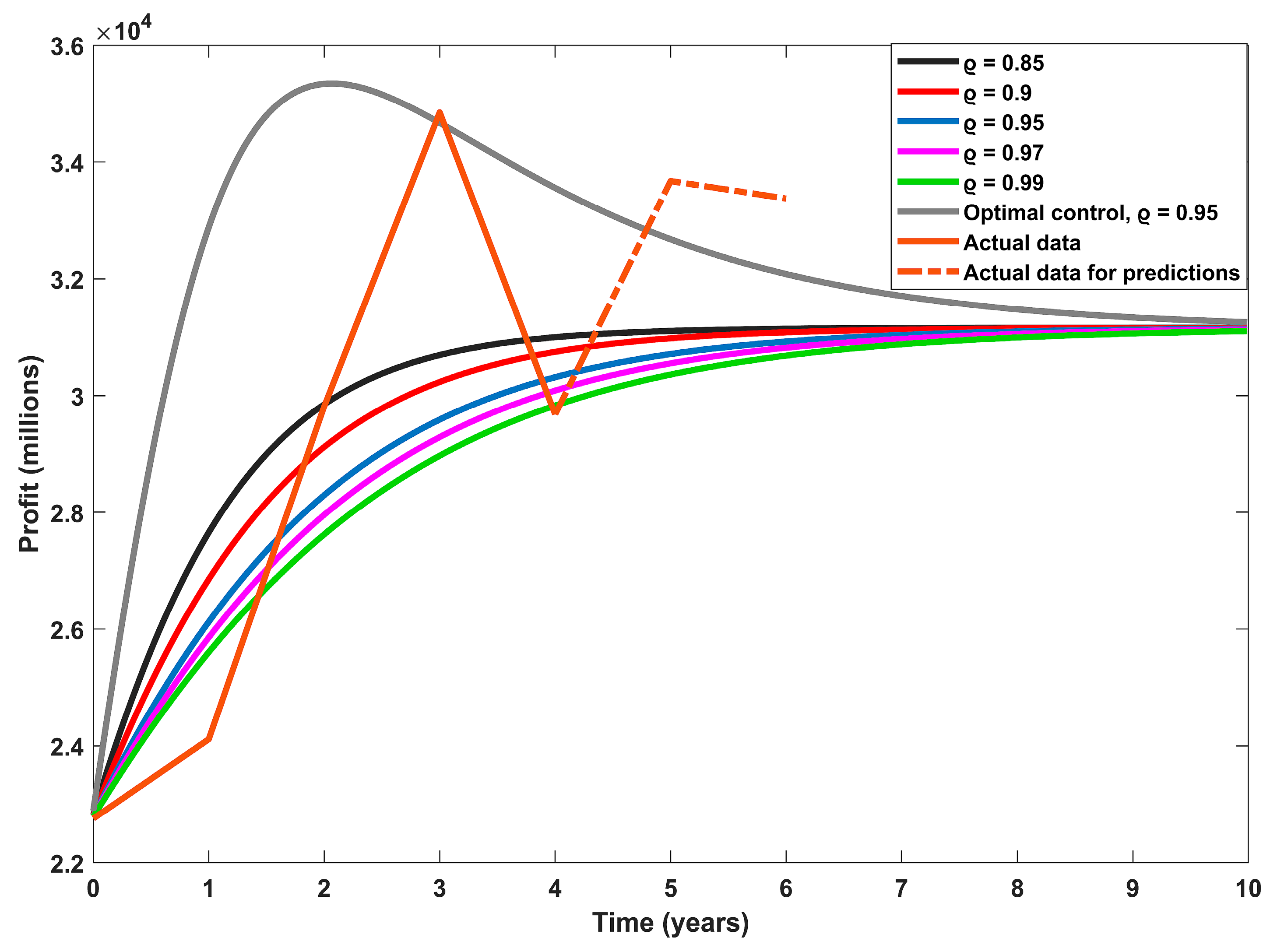
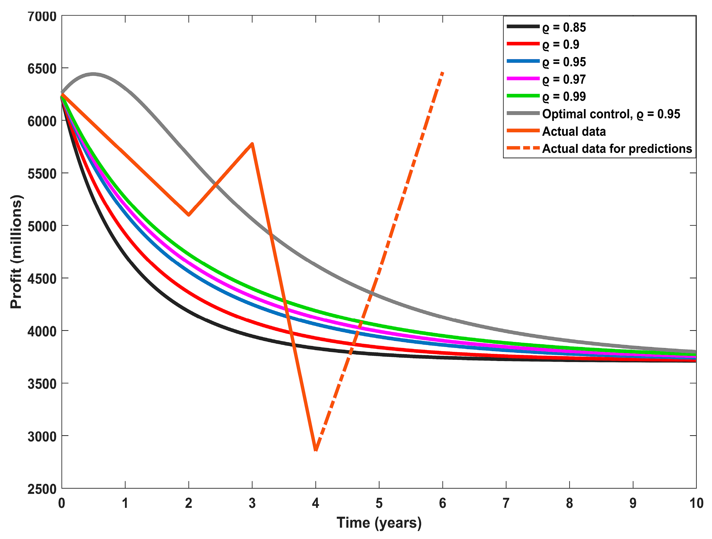
Starting with the public banks’ profits in million EGP, as indicated in Figure 1, the fractional orders 0.9, 0.95, and 0.97 give very near accuracy to describe this category, while both 0.85 and 0.99 have lower accuracy. Figure 2 depicts the dynamic behavior obtained by the second category, private and Arab banks. The fractional order 0.9 is the best, with the highest accuracy, followed by the fractional orders 0.85 and 0.95, while the fractional orders 0.97 and 0.99 present lower accuracy. In Figure 3, it is clearly shown that the fractional order 0.85 provides the best fit for the actual data of the third category of banks, and as we increase the fractional order, the accuracy starts to decrease. In the case of foreign banks, the fourth category, the fractional order 0.99 has the highest accuracy of fitting, as indicated in Figure 4. The fractional orders 0.97 and 0.95 have intermediate accuracy, while the fractional orders 0.9 and 0.85 are the worst for this category.
As is evident in all types of data for the four categories of banks, in the fifth year under study, 2020, the COVID-19 pandemic had a severe impact, causing a decrease in the profits of these banks and decreasing the efficiency of dynamic modeling. We therefore aimed to solve this problem: we developed the modeling process by presenting the second-fractional-order model by adding a specific optimal control function with a maximum value of the reinvestment varying from one category to another. The aim was to control the profits in order to absorb the occurrence of crises and so that the profits become as if they were without reinvestment in the absence of crises during a certain time interval. The proposed controlled dynamic model is solved numerically using the predefined Adams–Bashford scheme. We run the dynamic model with a fractional order parameter value of 0.95, as it gives intermediate accuracy for the four categories in the previously proposed model without control. The optimally controlled profits for the four categories are presented in Figure 1, Figure 2, Figure 3 and Figure 4. As presented, the controlling function has a strong impact on maximizing the banks’ profits.
The actual data of banks at the end of 2021 and 2022 [22,34,35] were used to check the proposed model’s ability to predict the banks’ profits. There was a significant decrease in the purchasing value of the EGP in 2022, and this was considered before using the available data for that year. As shown in Figure 1, the actual data of public banks in 2021 and 2022 depict profit values higher than predicted by the model, with a high percentage of error equal to 28%. This may be due to banks following different methods or policies than previously. When the actual data of private and Arabic banks are used and compared to the predicted value through the fractional model, as in Figure 2, the error of prediction is found to be 7.1%. Figure 3 shows that the proposed fractional model of order 0.95 succeeded in predicting the actual profit of foreign banks at the end of 2022 with zero error. The error describing the accuracy of prediction for the investment collaboration banks at the end of 2022 reached 63.5%, and this is the worst prediction error value. This means that some use of stochastic modeling to provide better accuracy in the predictions for this category is needed.

7. Conclusions

This paper concludes by modelling the profit competition of Egyptian banks through the derivation of a four-dimensional fractional-order competition model. We used the derived model to describe the competition between public banks, private and Arabic banks, foreign banks, and investment collaboration banks. Through an extended Adams–Bashford scheme, the established model is numerically solved with different fractional-order parameter values, trying to fit the available profit data. Based on the obtained results, the proposed model fitted the Egyptian banks’ profits with good accuracy except at the end of 2020, which suffered from a severe decrease in profits due to the COVID-19 pandemic. As a way of suggesting solutions to the sudden decrease in profits during crises, we created a reinvestment-control function as a proposal to introduce a pre-reinvestment-control system that can absorb this sudden decrease. After considering the controlling function, simulations were performed again, and the results show how the banks’ profits are controlled. In our future work, since crises cannot be expected, but rather fall within the scope of probability, we will consider the development of such models to contain enough stochasticity for the accurate dynamic prediction of banks’ profits.

Author Contributions

O.A.M.O.: Methodology, Software, Data curation, Writing—original draft. H.M.A.: Investigation, Conceptualization, Supervision. W.H.: Methodology, Formal analysis, Writing—original draft. All authors have read and agreed to the published version of the manuscript.

Funding

This research received no external funding.

Data Availability Statement

The data presented in this study are available on request from the corresponding author.

Conflicts of Interest

The authors declare no conflict of interest.

References

  1. Kahshan, M.; Lu, D.; Rahimi-Gorji, M. Hydrodynamical study of flow in a permeable channel: Application to flat plate dialyzer. Int. J. Hydrog. Energy 2019, 44, 17041–17047. [Google Scholar] [CrossRef]
  2. Uddin, S.; Mohamad, M.; Rahimi-Gorji, M.; Roslan, R.; Alarifi, I.M. Fractional electro-magneto transport of blood modeled with magnetic particles in cylindrical tube without singular kernel. Microsyst. Technol. 2019, 26, 405–414. [Google Scholar] [CrossRef]
  3. Michalakelis, C.; Christodoulos, C.; Varoutas, D.; Sphicopoulos, T. Dynamic estimation of markets exhibiting a prey–predator behavior. Expert Syst. Appl. 2012, 39, 7690–7700. [Google Scholar] [CrossRef]
  4. Lakka, S.; Michalakelis, C.; Varoutas, D.; Martakos, D. Competitive dynamics in the operating systems market: Modeling and policy implications. Technol. Forecast. Soc. Chang. 2013, 80, 88–105. [Google Scholar] [CrossRef]
  5. Atangana, A.; Gómez-Aguilar, J.F. Numerical approximation of riemann-liouville definition of fractional derivative: From riemann-liouville to atangana-baleanu. Numer. Methods Partial Differ. Equ. 2018, 34, 1502–1523. [Google Scholar] [CrossRef]
  6. Saad, K.M.; Khader, M.M.; Gómez-Aguilar, J.F.; Baleanu, D. Numerical solutions of the fractional fishers type equations with atangana-baleanu fractional derivative by using spectral collocation methods. Chaos Interdiscip. J. Nonlinear Sci. 2019, 29, 023116. [Google Scholar] [CrossRef]
  7. Solis-Perez, J.E.; Gómez-Aguilar, J.F. Variable-order fractalfractional time delay equations with power, exponential and mittag-leffler laws and their numerical solutions. Eng. Comput. 2020, 38, 555–577. [Google Scholar] [CrossRef]
  8. Safdari, H.; Aghdam, Y.E.; Gómez-Aguilar, J.F. Shifted chebyshev collocation of the fourth kind with convergence analysis for the space–time fractional advection-diffusion equation. Eng. Comput. 2020, 38, 1409–1420. [Google Scholar] [CrossRef]
  9. Atangana, A.; Gómez-Aguilar, J.F. Decolonisation of fractional calculus rules: Breaking commutativity and associativity to capture more natural phenomena. Eur. Phys. J. Plus 2018, 133, 166. [Google Scholar] [CrossRef]
  10. Gómez-Aguilar, J.F.; Yépez-Martínez, H.; Escobar-Jiménez, R.F.; Olivares-Peregrino, V.H.; Reyes, J.M.; Sosa, I.O. Series solution for the time-fractional coupled mkdv equation using the homotopy analysis method. Math. Probl. Eng. 2016, 2016, 7047126. [Google Scholar] [CrossRef]
  11. Omar, O.A.; Elbarkouky, R.A.; Ahmed, H.M. Fractional stochastic models for COVID-19: Case study of Egypt. Results Phys. 2021, 23, 104018. [Google Scholar] [CrossRef]
  12. Shikongo, A.; Nuugulu, S.M.; Elago, D.; Salom, A.T.; Owolabi, K.M. Fractional derivative operator on quarantine and isolation principle for COVID-19. In Advanced Numerical Methods for Differential Equations: Applications in Science and Engineering; Singh, H., Singh, J., Purohit, S.D., Kumar, D., Eds.; CRC Press: Boca Raton, FL, USA, 2021; pp. 205–226. [Google Scholar]
  13. Omar, O.A.; Alnafisah, Y.; Elbarkouky, R.A.; Ahmed, H.M. COVID-19 deterministic and stochastic modelling with optimized daily vaccinations in Saudi Arabia. Results Phys. 2021, 28, 104629. [Google Scholar] [CrossRef]
  14. Lu, J.; Ma, L. Numerical analysis of a fractional nonlinear oscillator with coordinate-dependent mass. Results Phys. 2022, 43, 106108. [Google Scholar] [CrossRef]
  15. Kumar, S.; Ghosh, S.; Samet, B.; Goufo, E.F.D. An analysis for heat equations arises in diffusion process using new Yang-Abdel-Aty-Cattani fractional operator. Math. Methods Appl. Sci. 2020, 43, 6062–6080. [Google Scholar] [CrossRef]
  16. Fatmawati; Khan, M.A.; Azizah, M.; Windarto; Ullah, S. A fractional model for the dynamics of competition between commercial and rural banks in Indonesia. Chaos Solitons Fractals 2019, 122, 32–46. [Google Scholar] [CrossRef]
  17. Wang, W.; Khan, M.A. Analysis and numerical simulation of fractional model of bank data with fractal-fractional atangana-baleanu derivative. J. Comput. Appl. Math. 2019, 369, 112646. [Google Scholar] [CrossRef]
  18. Gong, X.; Fatmawati; Khan, M.A. A new numerical solution of the competition model among bank data in caputo-fabrizio derivative. Alex. Eng. J. 2020, 59, 2251–2259. [Google Scholar] [CrossRef]
  19. Li, Z.; Liu, Z.; Khan, M.A. Fractional investigation of bank data with fractal-fractional caputo derivative. Chaos Solitons Fractals 2020, 131, 109528. [Google Scholar] [CrossRef]
  20. Qureshi, S.; Atangana, A. Mathematical analysis of dengue fever outbreak by novel fractional operators with field data. Phys. A Stat. Mech. Appl. 2019, 526, 121–127. [Google Scholar] [CrossRef]
  21. Qureshi, S.; Yusuf, A. Fractional derivatives applied to mseir problems: Comparative study with real world data. Eur. Phys. J. Plus 2019, 134, 171. [Google Scholar] [CrossRef]
  22. Central Bank of Egypt (CBE). Available online: https://www.cbe.org.eg/en/Pages/default.aspx (accessed on 10 February 2023).
  23. Kilbas, A.A.; Trujillo, J.J.; Srivastava, H.M. Theory and Applications of Fractional Differential Equations; Elsevier: Amsterdam, The Netherlands, 2006. [Google Scholar]
  24. Agrawal, O.P. Fractional variational calculus in terms of Riesz fractional derivatives. J. Phys. A 2007, 40, 6287–6303. [Google Scholar] [CrossRef]
  25. Zhu, C.; Yin, G. On competitive Lotka–Volterra model in random environments. J. Math. Anal. Appl. 2009, 357, 154–170. [Google Scholar] [CrossRef]
  26. Comes, C.A. Banking system: Three level Lotka-Volterra model. Procedia Econ. Finance 2012, 3, 251–255. [Google Scholar] [CrossRef]
  27. Omar, O.A.; Elbarkouky, R.A.; Ahmed, H.M. Fractional stochastic modelling of COVID-19 under wide spread of vaccinations: Egyptian case study. Alex. Eng. J. 2022, 61, 8595–8609. [Google Scholar] [CrossRef]
  28. Precup, R. Theorems of Leray-Schauder Type and Applications; CRC Press: Boca Raton, FL, USA, 2002. [Google Scholar]
  29. Ye, H.; Gao, J.; Ding, Y. A generalized Gronwall inequality and its application to a fractional differential equation. J. Math. Anal. Appl. 2007, 328, 1075–1081. [Google Scholar] [CrossRef]
  30. Sharp, R.S.; Peng, H. Vehicle dynamics applications of optimal control theory. Veh. Syst. Dyn. 2011, 49, 1073–1111. [Google Scholar] [CrossRef]
  31. Atangana, A.; Owolabi, K.M. New numerical approach for fractional differential equations. Math. Model. Nat. Phenom. 2021, 16, 47. [Google Scholar] [CrossRef]
  32. Biala, T.; Jator, S.N. Block backward differentiation formulas for fractional differential equations. Int. J. Eng. Math. 2015, 2015, 650425. [Google Scholar] [CrossRef]
  33. Zabidi, N.A.; Majid, Z.A.; Kilicman, A.; Ibrahim, Z.B. Numerical solution of fractional differential equations with Caputo derivative by using numerical fractional predict–correct technique. Adv. Contin. Discret. Model. 2022, 2022, 26. [Google Scholar] [CrossRef]
  34. FirstBank Indicator. Indicators of Financial Performance of Egyptian Banks. Available online: https://www.firstbankeg.com (accessed on 9 June 2023).
  35. Almal Daily Egyptian Newspaper. Available online: https://almalnews.com (accessed on 9 June 2023).
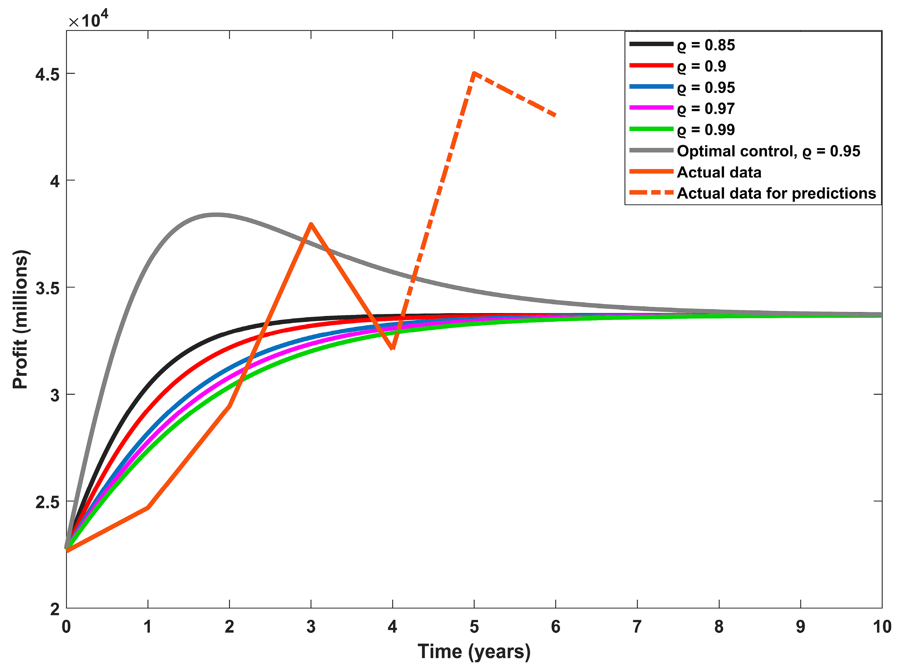
Figure 1. Public banks’ dynamic profits in million EGP.
Fractalfract 07 00473 g001
Figure 2. Private and Arab banks’ dynamic profits in million EGP.
Fractalfract 07 00473 g002
Figure 3. Foreign banks’ dynamic profits in million EGP.
Fractalfract 07 00473 g003
Figure 4. Investment collaboration banks’ dynamic profits in million EGP.
Fractalfract 07 00473 g004
Table 1. Dynamic models’ estimated parameters.
Parameter NameSymbolEstimated Value
Public banks’ growth rate μ 1 0.7
Private and Arab banks’ growth rate μ 2 0.5
Foreign banks’ growth rate μ 3 0.45
Investment collaboration banks’ growth rate μ 4 0.3
Public banks’ max. profit η 1 33,696
Private and Arab banks’ max. profit η 2 31,162
Foreign banks’ max. profit η 3 11,679
Investment collaboration banks’ max. profit η 4 3710
Public banks’ competition parameter γ 1 1.9 × 10⁻¹⁸
Private and Arab banks’ competition parameter γ 2 2.3 × 10⁻¹⁸
Foreign banks’ competition parameter γ 3 1.02 × 10⁻¹⁸
Investment collaboration competition parameter γ 4 5 × 10⁻¹⁸
Public banks’ max. level of investment c 1 0.392
Private and Arab banks’ max. level of investment c 2 0.327
Foreign banks max. level of investment c 3 0.245
Investment collaboration banks’ max. level of investment c 4 0.295
Disclaimer/Publisher’s Note: The statements, opinions and data contained in all publications are solely those of the individual author(s) and contributor(s) and not of MDPI and/or the editor(s). MDPI and/or the editor(s) disclaim responsibility for any injury to people or property resulting from any ideas, methods, instructions or products referred to in the content.