Article

Block-Centered Finite-Difference Methods for Time-Fractional Fourth-Order Parabolic Equations

School of Mathematics and Statistics, Shandong Normal University, Jinan 250358, China
*
Author to whom correspondence should be addressed.
Fractal Fract. 2023, 7(6), 471; https://doi.org/10.3390/fractalfract7060471
Submission received: 10 May 2023 / Revised: 7 June 2023 / Accepted: 9 June 2023 / Published: 14 June 2023

Abstract

:
The block-centered finite-difference method has many advantages, and the time-fractional fourth-order equation is widely used in physics and engineering science. In this paper, we consider variable-coefficient fourth-order parabolic equations of fractional-order time derivatives with Neumann boundary conditions. The fractional-order time derivatives are approximated by L 1 interpolation. We propose the block-centered finite-difference scheme for fourth-order parabolic equations with fractional-order time derivatives. We prove the stability of the block-centered finite-difference scheme and the second-order convergence of the discrete L 2 norms of the approximate solution and its derivatives of every order. Numerical examples are provided to verify the effectiveness of the block-centered finite-difference scheme.

1. Introduction

The block-centered finite-difference method was first applied to the simulation of oil reservoirs [1]. Russell and Wheeler [1] proved that the block-centered finite-difference method is equivalent to the mixed finite-element method with a special numerical quadrature formula. Based on this equivalence, it is easier to discuss the stability and convergence of the block-centered finite-difference method. In addition, the block-centered finite-difference method can simultaneously approximate the exact solution of the original problem and its derivatives, thus preserving the local conservation of the problem. Moreover, for problems with Neumann boundary conditions, the numerical solution of nodes near the boundary does not need to be considered separately. On this basis, Weiser and Wheeler [2] introduced the block-centered finite-difference method for linear self-adjoint and non-self-adjoint elliptic and parabolic problems with Neumann boundary conditions in a rectangular area. They proved that the errors of the discrete L2 norms for the solution and the first derivative are both of the second order. Refs. [3,4,5] considered the block-centered finite-difference method for the nonlinear Darcy–Forchheimer equation. The block-centered finite-difference method on non-uniform grids has been discussed in [6,7,8,9,10,11]. In [12], Ren and Zhang studied the Crank–Nicolson block-centered difference method for solving linear parabolic equations in bounded domains. Li and Rui [13] introduced and analyzed the block-centered finite-difference method for distributed-order time-fractional diffusion-wave equations with Neumann boundary conditions. In addition, [14,15,16,17,18] discussed the two-grid and parallel block-centered finite-difference schemes for parabolic equations and diffusion equations with fractional-order time derivatives. The resulting schemes have a second-order accuracy in space and a ( 2 α ) -order accuracy in time, and the unconditional stability and convergence have been proved theoretically. In [19], Shi and Xie derived and analyzed the fourth-order compact block-centered finite-difference schemes for one-dimensional and two-dimensional variable-coefficient elliptic and parabolic problems. They demonstrated the stability of the solution and flux and performed optimal fourth-order error estimation.
The fourth-order parabolic problem has important practical significance in science and engineering. It can be used to describe bistable phenomena encountered in various fields [20], such as the competition and spatial sorting of biological populations, migration of riverbeds, charge-density distribution of quantum semiconductors, etc. [21,22]. Since the exact solution of the fourth-order equation is difficult to obtain, the numerical method of the fourth-order parabolic equation has attracted extensive attention from researchers in recent years. In [22], Jüngel studied the positivity-preserving numerical scheme for a class of fourth-order nonlinear parabolic systems in quantum semiconductor modeling and performed transient calculations using a macroscopic quantum model for the first time. The time-fractional derivative is especially good at describing dynamic processes with history dependence; therefore, the time-fractional differential equation can be used to depict physical problems with time variables with great accuracy such as in [23,24]. Fractional Caputo derivatives can be used to study the dynamics of plankton–fish models in the presence of toxic compounds produced by harmful algal blooms [25]. The time-fractional fourth-order parabolic equation can better describe the propagation of waves in intense laser beams and the charge-density distribution of quantum semiconductors. Currently, many researchers are dedicated to the study of fractional-order differential equations. Aziz [26] studied two inverse source problems of fourth-order parabolic equations with fractional time derivatives. Li and Liao [27] used a class of L 1 -Galerkin finite-element methods to study the numerical solution of time-fractional nonlinear parabolic problems. They provided the optimal error estimates of several fully discrete linearized Galerkin finite-element methods for solving nonlinear problems. The authors of [28] established a fully discrete weak Galerkin finite-element method for the initial boundary value problems of two-dimensional sub-diffusion equations with Caputo fractional time derivatives. In [29], Liu and Du proposed and discussed the finite-difference/finite-element method for solving nonlinear time-fractional fourth-order reaction and diffusion problems. A new implicit compact difference scheme for fourth-order fractional diffuse wave systems was constructed in [30]. In addition, Ji and Sun [31] studied the compact algorithm for a class of fourth-order fractional diffusion equations with first-order Dirichlet boundary conditions.
So far, no block-centered finite-difference methods for fourth-order parabolic equations with fractional-order time derivatives have been published in the literature. For the Neumann boundary conditions, which provide the boundary charge density, the time fractional fourth-order parabolic equation is more suitable to be solved using the block-centered finite-difference method, without separately considering the numerical solution of the nodes near the boundary. Therefore, it is of great theoretical and practical significance to propose and develop a block-centered finite-difference method for time-fractional fourth-order parabolic equations. This paper discusses the block-centered finite-difference method [30] for variable-coefficient fourth-order parabolic equations of fractional-order time derivatives with Neumann boundary conditions. In this method, the mixed finite-element method is used for theoretical analysis, which gives the error analysis a certain regularity. The fractional-order time derivatives are approximated by L 1 interpolation. The block-centered finite-difference scheme is established, and the error estimations of the discrete L 2 norm of the approximate solution and its derivatives are provided. Numerical examples are presented to verify the effectiveness of the block-centered finite-difference scheme.
This paper is organized as follows. Section 2 introduces the notations used in this paper. Section 3 presents the block-centered finite-difference scheme and error estimation for fourth-order ordinary differential equations. Section 4 establishes the block-centered finite-difference schemes for the fractional-order time derivatives and proves the stability and convergence of the schemes. In 
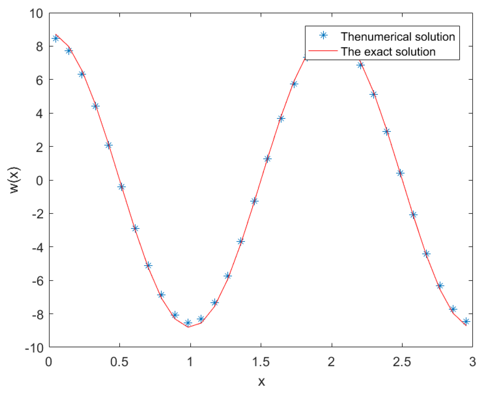
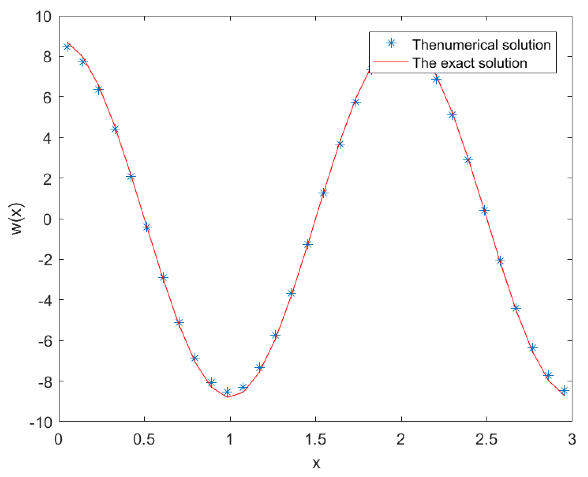
Section 5, numerical examples are provided to verify the convergence of the proposed schemes.

2. Notations

We first introduce some notations and definitions used in this paper, which will help with the following analysis. We use notations similar to those in [2]. Define the partition T x of Ω = ( x L , x R ) as
T x : x L = x 1 / 2 < x 3 / 2 < < x N 1 / 2 < x N + 1 / 2 = x R .
For each i = 1 to N, define
x i = 1 2 ( x i + 1 / 2 + x i 1 / 2 ) , h i = x i + 1 / 2 x i 1 / 2 , h = max i h i , h i + 1 / 2 = x i + 1 x i = 1 2 ( h i + h i + 1 ) , Ω i = ( x i 1 / 2 , x i + 1 / 2 ) .
The block-centered dual partition grids are defined as T x * = { x i } .
Take a positive integer J, and let τ = T ^ / J , t n = n τ ( 0 n J ) .
For any function g ( x ) , let g i , g i + 1 / 2 , g i n donate g ( x i ) , g ( x i + 1 / 2 ) , g ( x i , t n ) .
Define the following notations
[ d x g ] i + 1 / 2 = g i + 1 g i h i + 1 / 2 ,
[ D x g ] i = g i + 1 / 2 g i 1 / 2 h i .
For functions F and G, define the midpoint quadrature formula and trapezoidal quadrature formula on Ω i as
( F , G ) M , Ω i = h i F ( x i ) G ( x i ) ,
and
( F , G ) T , Ω i = h i 2 [ F ( x i 1 / 2 ) G ( x i 1 / 2 ) + F ( x i + 1 / 2 ) G ( x i + 1 / 2 ) ] .
Given functions f ( x ) and g ( x ) , define the L 2 inner product and norm
( f , g ) = Ω f ( x ) g ( x ) d x , f 2 = ( f , f ) ,
and the discrete L 2 inner products and norms
( f , g ) M = i = 1 N h i f i g i , f M 2 = ( f , f ) M , ( f , g ) T = i = 1 N h i + 1 / 2 f i + 1 / 2 g i + 1 / 2 , f T 2 = ( f , f ) T , f L ( Ω ) = max 1 i N | f ( x i ) | .
Define S c d ( T x ) as the finite-dimensional space of one-dimensional functions that have c continuous derivatives on ( x L , x R ) and are piecewise polynomials of degree d in each interval Ω i . When c = 1 , the functions themselves may be discontinuous.
The notation g = O ( h k ) , k > 0 means that there exists a constant C such that g ( x ) C h k as h approaches zero.

3. Fourth-Order Ordinary Differential Equation

In order to discuss the block-centered difference method for the time-fractional fourth-order parabolic equation, we first consider the block-centered difference scheme for the fourth-order ordinary differential equation.
We consider fourth-order variable-coefficient ordinary differential equations with Neumann boundary conditions
( a ( x ) w ) = f ( x ) , x ( x L , x R ) , w | x = x L = 0 , w | x = x R = 0 , ( a ( x ) w ) | x = x L = 0 , ( a ( x ) w ) | x = x R = 0 .
where f ( x ) is a known smooth function.
Let
v ( x ) = w ( x ) , p ( x ) = a ( x ) v ( x ) , u ( x ) = p ( x ) ,
then, we have
u ( x ) = f ( x ) , x ( x L , x R ) , u ( x ) = p ( x ) , a ( x ) v ( x ) = p ( x ) , v ( x ) = w ( x ) , u ( x ) = 0 , v ( x ) = 0 , a t x = x L , x = x R .
The block-centered finite-difference approximations U i + 1 / 2 , V i + 1 / 2 , W i , and P i to u ( x i + 1 / 2 ) , v ( x i + 1 / 2 ) , w ( x i ) , and p ( x i ) ( i = 1 , 2 , , N ) , respectively, satisfy the following
[ D x U ] i = f i , U 1 / 2 = 0 , U N + 1 / 2 = 0 ,
U i + 1 / 2 = [ d x P ] i + 1 / 2 ,
[ D x V ] i = P i a i , V 1 / 2 = 0 , V N + 1 / 2 = 0 ,
V i + 1 / 2 = [ d x W ] i + 1 / 2 ,
which approximate the original Equation (2). The above block-centered finite-difference scheme can be written as a mixed finite-element scheme with approximate integration
( ( U ) , 1 ) Ω i = ( f , 1 ) M , Ω i ,
( U , χ ) T ( P , χ ) = 0 , χ S ˜ ,
( ( V ) , 1 ) Ω i = ( P a , 1 ) M , Ω i ,
( V , χ ) T ( W , χ ) = 0 , χ S ˜ .
where S ˜ = S 0 1 ( T x ) { χ : χ ( x L ) = χ ( x R ) = 0 } , U and V are in S ˜ , and P and W are in S 1 0 ( T x ) .
 Lemma 1 
([2]). If w ( 5 ) ( x ) is continuous and f ( x ) is in L 1 ( Ω i ) for all i,
U u T = O ( h 2 ) , P p M = O ( h 2 ) , V v T = O ( h 2 ) , W w M = O ( h 2 ) .
 Proof.
By using Equations (2)–(6) and the Taylor expansion, we can obtain
u i + 1 / 2 U i + 1 / 2 = x 1 / 2 x i + 1 / 2 ( u U ) d x = x 1 / 2 x i + 1 / 2 ( f ( x ) f ( x i ) ) d x = j = 1 i Ω j ( f ( x ) f ( x j ) ) d x = j = 1 i Ω j ( ( x x j ) f j + ( x x j ) 2 2 f j + x j x ( x s ) 2 2 f ( s ) d s ) d x = j = 1 i ( 1 24 h j 3 f j + Ω j x j x ( x s ) 2 2 f ( s ) d s d x ) 1 24 j = 1 i h j 3 f j + | j = 1 i Ω j x j x ( x s ) 2 2 f ( s ) d s d x | 1 24 j = 1 i h j 3 f j + j = 1 i h j 3 8 Ω j | f | d x .
Then, we have
| u i + 1 / 2 U i + 1 / 2 | j = 1 i h j 2 2 f L 1 .
p i + 1 P i + 1 = j = 1 i x j x j + 1 ( u U j + 1 / 2 ) d x 0 x 1 u d x = 0 x 1 u d x + j = 1 i x j x j + 1 ( U u ) j + 1 / 2 d x + j = 1 i x j x j + 1 ( u j + 1 / 2 u ) d x .
According to Equation (12), the first two terms on the right side of the equation are O ( h 2 ) . Now, we estimate the third term on the right side.
j = 1 i x j x j + 1 ( p j + 1 / 2 p ) d x = j = 1 i x j x j + 1 ( ( x x j + 1 / 2 ) p j + 1 / 2 + x j + 1 / 2 x ( x s ) p ( s ) d s ) d x | j = 2 i h j 2 8 | p j + 1 / 2 p j 1 / 2 | + h 1 2 8 | p 3 / 2 | + h i + 1 2 8 | p i + 1 / 2 | + j = 1 i h j 2 2 x j x j + 1 | p | d s = O ( h 2 ) .
We can obtain
| p i + 1 P i + 1 | = O ( h 2 ) .
Similarly, we can reach the same conclusion for V and W by employing the Taylor expansion. □
The second-order error estimation for a block-centered difference scheme applied to fourth-order ordinary differential equations has been derived.

4. Time-Fractional Fourth-Order Parabolic Equation

In this section, we consider the block-centered finite-difference method for a time-fractional fourth-order parabolic equation when 0 < α < 1 .
We consider the following variable-coefficient fractional fourth-order parabolic problem with initial and boundary value conditions
0 c D t α w ( x , t ) + μ 2 x 2 ( a ( x ) 2 w ( x , t ) x 2 ) = f ( x , t ) , x ( x L , x R ) , t ( 0 , T ^ ] , w ( x , 0 ) = φ ( x ) , x ( x L , x R ) , t ( 0 , T ^ ] , w ( x , t ) x | x = x L = 0 , w ( x , t ) x | x = x R = 0 , t ( 0 , T ^ ] , x ( a ( x ) 2 w ( x , t ) x 2 ) | x = x L = 0 , x ( a ( x ) 2 w ( x , t ) x 2 ) | x = x R = 0 , t ( 0 , T ^ ] .
where μ is a constant; a ( x ) , f ( x , t ) , and φ ( x ) are known smooth functions; and it is assumed that 0 < a 0 a ( x ) a 1 .
We consider the case 0 < α < 1 . 0 c D t α w in (13) is defined as the Caputo fractional derivative of α , which is given by
0 c D t α w ( x , t ) = 1 Γ ( 1 α ) 0 t ( t τ ) α w ( x , τ ) τ d τ .

4.1. Block-Centered Finite-Difference Scheme

In this subsection, we provide the block-centered difference scheme for a time-fractional fourth-order parabolic equation.
 Lemma 2 
([32]). Suppose f ( t ) C 2 [ 0 , T ^ ] , 0 < α < 1 ,
0 c D t α f ( t n ) = D τ α f ( t n ) + R ( f ( t n ) ) = τ α Γ ( 2 α ) [ a 0 ( α ) f ( t n ) k = 1 n 1 ( a n k 1 ( α ) a n k ( α ) ) f ( t k ) a n 1 ( α ) f ( t 0 ) ] + R ( f ( t n ) ) ,
where
a k ( α ) = ( k + 1 ) 1 α k 1 α , | R ( f ( t n ) ) | 1 2 Γ ( 1 α ) [ 1 4 + α ( 1 α ) ( 2 α ) ] max t 0 t t n | f ( t ) | τ 2 α .
 Lemma 3 
([32]). Given that 0 < α < 1 , we have l i m l + a l = 0 ,
1 = a 0 ( α ) > a 1 ( α ) > a 2 ( α ) > > a l ( α ) > 0 .
The block-centered finite-difference method (13) defines { U i + 1 / 2 n } n = 1 M , { V i + 1 / 2 n } n = 1 M , { W i n } n = 1 M and { P i n } n = 1 M ( i = 1 , 2 , , N ) , satisfying
[ D τ α W ] i n + μ [ D x U ] i n = f i n , α ( 0 , 1 ) , U 1 / 2 n = 0 , U N + 1 / 2 n = 0 ,
U i + 1 / 2 n = [ d x P ] i + 1 / 2 n ,
[ D x V ] i n = P i n a i , V 1 / 2 n = 0 , V N + 1 / 2 n = 0 ,
V i + 1 / 2 n = [ d x W ] i + 1 / 2 n ,
where U 0 = E h u 0 , P 0 = E h p 0 , V 0 = E h v 0 , and W 0 = E h w 0 . Here, U i + 1 / 2 n , P i n , V i + 1 / 2 n , and W i n are approximations to u i + 1 / 2 n , p i n , v i + 1 / 2 n , and w i n , respectively, and E h u n , E h p n , E h v n , and E h w n are their corresponding elliptic projections.
The above block-centered finite-difference scheme can be written as a mixed finite-element scheme with approximate integration
( D τ α W n , 1 ) Ω i + μ ( ( U n ) , 1 ) Ω i = ( f n , 1 ) M , Ω i , α ( 0 , 1 ) ,
( U n , χ ) T ( P n , χ ) = 0 , χ S ˜ ,
( ( V n ) , 1 ) Ω i = ( P n a , 1 ) M , Ω i ,
( V n , χ ) T ( W n , χ ) = 0 , χ S ˜ .

4.2. Stability Analysis

In this subsection, we prove the stability of the scheme (14)–(17) when 0 < α < 1 .
 Theorem 1.
For the block-centered difference scheme, the following stable inequality holds unconditionally for sufficiently small τ
W n M C 1 W 0 M + C 2 max 1 k J f k M .
 Proof. 
For n = 1 , by multiplying (14) by h i W i 1 and summing on i from 1 to N, we obtain ( D τ α W 1 , W 1 ) M + μ ( W x x 1 , W x x 1 ) M = ( f 1 , W 1 ) M . So,
( a 0 ( α ) W 1 , W 1 ) M ( a 0 ( α ) W 0 , W 1 ) M + ρ ( f 1 , W 1 ) M ,
where ρ = τ α Γ ( 2 α ) . Using the Cauchy–Schwarz inequality and Young inequality, we can obtain
( 1 ρ 2 ) W 1 M 2 W 0 M 2 + 2 ρ f 1 M 2 .
So, we have
W 1 M 2 2 2 ρ W 0 M 2 + 4 ρ 2 ρ f 1 M 2 .
Thus, we can obtain
W 1 M C 1 W 0 M + C 2 f 1 M .
For n 2 , we suppose that the stability conclusion of the difference scheme is valid when k n 1 .
Then, by multiplying (14) by h i W i n and summing on i from 1 to N, we can obtain ( D τ α W n , W n ) M ( f n , W n ) M . So,
( a 0 ( α ) W n , W n ) M ( k = 1 n 1 ( a n k 1 ( α ) a n k ( α ) ) W k , W n ) M + ( a n 1 ( α ) W 0 , W n ) M + ρ ( f n , W n ) M .
Using the Cauchy–Schwarz inequality and Young inequality, we obtain
W n M 2 2 2 ρ k = 1 n 1 ( a n k 1 ( α ) a n k ( α ) ) W k M 2 + 2 2 ρ a n 1 ( α ) W 0 M 2 + 4 ρ 2 ρ f n M 2 .
Through mathematical induction and using the relation of coefficient a k , we have
W n M 2 2 2 ρ k = 1 n 1 ( a n k 1 ( α ) a n k ( α ) ) ( C 1 W 0 M 2 + C 2 max 1 k J f k M 2 ) + 2 2 ρ a n 1 ( α ) W 0 M 2 + 4 ρ 2 ρ f n M 2 2 2 ρ [ ( C 1 ( a 0 ( α ) a n 1 ( α ) ) + a n 1 ( α ) ) W 0 M 2 + ( C 2 ( a 0 ( α ) a n 1 ( α ) ) + 2 ρ ) max 1 k J f k M 2 ] .
There are constants C 3 and C 4 that make
W n M 2 C 3 W 0 M 2 + C 4 max 1 k J f k M 2 .
So, we can obtain
W n M C 1 W 0 M + C 2 max 1 k J f k M .
We complete the proof. □

4.3. Error Analysis

The error analysis of the block-centered difference scheme for the time-fractional parabolic equation is performed.
Error estimates for the finite-difference scheme of (14)–(17) are derived using a technique of mixed finite-element methods for parabolic partial differential equations.
μ 2 x 2 ( a ( x ) 2 w n x 2 ) = ϕ = f n 0 c D t α w n , α ( 0 , 1 ) , x ( x L , x R ) ,
w n x | x = x L = 0 , w n x | x = x R = 0 ,
x ( a ( x ) 2 w n x 2 ) | x = x L = 0 , x ( a ( x ) 2 w n x 2 ) | x = x R = 0 .
For fixed n, let E h u i + 1 / 2 n , E h v i + 1 / 2 n , E h w i n , and E h p i n be defined by
μ [ D x E h u ] i n = f i n ( 0 c D t α w ) i n , E h u 1 / 2 n = 0 , E h u N + 1 / 2 n = 0 ,
E h u i + 1 / 2 n = [ d x E h p ] i + 1 / 2 n ,
[ D x E h v ] i n = E h p i n a i , E h v 1 / 2 n = 0 , E h v N + 1 / 2 n = 0 ,
E h v i + 1 / 2 n = [ d x E h w ] i + 1 / 2 n ,
where E h u 0 = ( a ( x ) φ ( x ) ) , E h p 0 = a ( x ) φ ( x ) , E h v 0 = φ ( x ) , and E h w 0 = φ ( x ) .
Equations (25)–(28) can be written as a mixed finite-element method with approximate integration
μ ( ( E h u n ) , 1 ) Ω i = ( f n , 1 ) M , Ω i ( 0 c D t α w n , 1 ) M , Ω i ,
( E h u n , χ ) T ( E h p n , χ ) = 0 , χ S ˜ ,
( ( E h v n ) , 1 ) Ω i = ( E h p n a , 1 ) M , Ω i ,
( E h v n , χ ) T ( E h w n , χ ) = 0 , χ S ˜ .
By the error of the ellipse projection, we have
E h u n u n T = O ( h 2 ) , E h p n p n M = O ( h 2 ) , E h v n v n T = O ( h 2 ) , E h w n w n M = O ( h 2 ) ,
which hold for sufficiently smooth w.
By differentiating t in Equations (25)–(28), we can obtain the following estimation
E h w t n w t n M = O ( h 2 ) .
Set ξ i + 1 / 2 n = U i + 1 / 2 n E h u i + 1 / 2 n , η i n = P i n E h p i n , θ i + 1 / 2 n = V i + 1 / 2 n E h v i + 1 / 2 n , ζ i n = W i n E h w i n , and σ i n = E h w i n w i n .
By subtracting (25) from (14), we obtain
D τ α ζ i n + μ [ D x ξ ] i n = R ( w i n ) D τ α σ i n , α ( 0 , 1 ) , ξ 1 / 2 n = 0 , ξ N + 1 / 2 n = 0 .
By subtracting (26), (27) and (28) from (15), (16) and (17), respectively, we obtain
ξ i + 1 / 2 n = [ d x η ] i + 1 / 2 n ,
η i n = a i [ D x θ ] i n , θ 1 / 2 n = 0 , θ N + 1 / 2 n = 0 ,
θ i + 1 / 2 n = [ d x ζ ] i + 1 / 2 n .
By multiplying (35) by h i ζ i n and summing on i from 1 to N, we deduce that
( D τ α ζ n , ζ n ) M + μ ( D x ξ n , ζ n ) M = ( R ( w n ) , ζ n ) M ( D τ α σ n , ζ n ) M .
By (36)–(38), and Lemma 2, we have
( D x ξ n , ζ n ) M = ( D x ( d x η n ) , ζ n ) M = ( d x η n , d x ζ n ) T = ( η n , D x θ n ) M = 1 a ( η n , η n ) M .
Now,
( D τ α ζ n , ζ n ) M = τ α Γ ( 2 α ) [ a 0 ( α ) ( ζ n , ζ n ) M k = 1 n 1 ( a n k 1 ( α ) a n k ( α ) ) ( ζ k , ζ n ) M a n 1 ( α ) ( ζ 0 , ζ n ) M ] .
Let ρ = τ α Γ ( 2 α ) , and (39) can be written as
ζ n M 2 + μ ρ a 1 η n M 2 k = 1 n 1 ( a n k 1 ( α ) a n k ( α ) ) ( ζ k , ζ n ) M + a n 1 ( α ) ( ζ 0 , ζ n ) M + ρ | ( R ( w n ) , ζ n ) M | + ρ | ( D τ α σ n , ζ n ) M | .
By the Cauchy–Schwarz inequality and Young inequality, we have
( 1 ρ 2 ) ζ n M 2 + 2 a 1 μ ρ η n M 2 k = 1 n 1 ( a n k 1 ( α ) a n k ( α ) ) ζ k M 2 + a n 1 ( α ) ζ 0 M 2 + 4 ρ D τ α σ n M 2 + 4 ρ R ( w n ) M 2 .
According to the definition of the fractional derivative and Equation (34),
D τ α σ n M = 1 Γ ( 1 α ) k = 1 n σ k σ k 1 τ t k 1 t k ( t n t ) α d t M = 1 Γ ( 1 α ) k = 1 n 1 τ t k 1 t k σ t d t t k 1 t k ( t n t ) α d t M 1 Γ ( 1 α ) max 0 t t n σ t M k = 1 n t k 1 t k ( t n t ) α d t T 1 α Γ ( 2 α ) max 0 t t n σ t M C h 2 .
Notice that ζ 0 = 0 . Using Theorem 1 and the inductive hypothesis, we deduce that
( 1 ρ 2 ) ζ n M 2 + 2 a 1 μ ρ η n M 2 C ( τ 4 2 α + h 4 ) .
Thus, we have
ζ n M 2 C ( τ 4 2 α + h 4 ) ,
η n M 2 C ( τ 4 2 α + h 4 ) .
By multiplying (35) by h i η i n and summing on i from 1 to N, we can obtain
( D τ α ζ n , η n ) M + μ ( D x ξ n , η n ) M = ( R ( w n ) , η n ) M ( D τ α σ n , η n ) M .
Now,
( D τ α ζ n , η n ) M = τ α Γ ( 2 α ) [ a 0 ( α ) ( ζ n , η n ) M k = 1 n 1 ( a n k 1 ( α ) a n k ( α ) ) ( ζ k , η n ) M a n 1 ( α ) ( ζ 0 , η n ) M ] .
By using (36)–(38), and Lemma 2, we derive
( ζ n , η n ) M = a ( θ n , θ n ) T ,
( D x ξ n , η n ) M = ( ξ n , ξ n ) T .
By substituting (49)–(51) into (48), (48) can be deformable to
a 0 θ n T 2 + μ ρ ξ n T 2 a 1 k = 1 n 1 ( a n k 1 ( α ) a n k ( α ) ) ( θ k , θ n ) T + a 1 a n 1 ( α ) ( θ 0 , θ n ) T + ρ | ( R ( w n ) , η n ) M | + ρ | ( D τ α σ n , η n ) M | .
By the Cauchy–Schwarz inequality, we derive
( 2 a 0 a 1 ) θ n T 2 + 2 μ ρ ξ n T 2 a 1 k = 1 n 1 ( a n k 1 ( α ) a n k ( α ) ) θ k T 2 + a 1 a n 1 ( α ) θ 0 T 2 + 2 ρ η n M 2 + ρ D τ α σ n M 2 + ρ R ( w n ) M 2 .
Similarly, when 2 a 0 > a 1 , using the above mathematical induction and substituting (44) and (47) into (53), we can obtain
( 2 a 0 a 1 ) θ n T 2 + 2 μ ρ ξ n T 2 C ( τ 4 2 α + h 4 ) .
So, we can obtain
θ n T 2 C ( τ 4 2 α + h 4 ) ,
ξ n T 2 C ( τ 4 2 α + h 4 ) .
By (33) and the triangle inequality,
U n u n T 2 C ( τ 4 2 α + h 4 ) , P n p n M 2 C ( τ 4 2 α + h 4 ) ,
V n v n T 2 C ( τ 4 2 α + h 4 ) , W n w n M 2 C ( τ 4 2 α + h 4 ) ,
which hold for sufficiently smooth w.
We can draw the following conclusion.
 Theorem 2.
Let w be sufficiently smooth and satisfy (13). If U, P, V, and W satisfy (14)–(17), for all n , n = 1 , 2 , , J ,
U n u n T = O ( τ 2 α + h 2 ) , P n p n M = O ( τ 2 α + h 2 ) ,
V n v n T = O ( τ 2 α + h 2 ) , W n w n M = O ( τ 2 α + h 2 ) .

5. Numerical Experiments

In this section, we present three numerical examples to verify the effectiveness and convergence of the block-centered finite-difference method.
 Example 1.
Consider the following fourth-order ordinary differential equation
w = f ( x ) , x ( 0 , 1 ) , w | x = 0 = 0 , w | x = 1 = 0 , x ( 0 , 1 ) , w | x = 0 = 0 , w | x = 1 = 0 , x ( 0 , 1 ) .
We provide the exact solution to the problem w ( x ) = cos ( π x ) and a source term f ( x ) = π 4 cos ( π x ) .
The original equation is discretized by the block-centered difference scheme, resulting in Equations (3)–(6). Equations (4)–(6) are substituted into Equation (3) to form a system of linear equations about the unknown function W. The approximate solution of W is obtained using MATLAB software, whereas the approximate solutions of V, P, and U are obtained using Equations (4)–(6).
Take the spatial step h = 1 / N . The space errors and convergence orders of W, V, P, and U are shown in Table 1, Table 2, Table 3 and Table 4, respectively. The second and fourth columns in Table 1, Table 2, Table 3 and Table 4 show the maximum norm error and discrete L2 norm error, respectively, whereas the third and fifth columns show their corresponding spatial convergence orders, respectively. It can be seen from the table that the order of spatial convergence reaches the second order for both the maximum norm and discrete L2 error, which verifies the convergence of the block-centered finite-difference scheme.
For the functions S ( x ) and s ( x ) , L E r r o r and L 2 E r r o r , as defined below, are used
S s L ( Ω ) = max 1 i N | S ( x i ) s ( x i ) | , S s L 2 ( Ω ) = ( i = 1 N | S ( x i ) s ( x i ) | 2 h ) 1 / 2 .
Figure 1 illustrates the numerical solution and the exact solution when L = 3 . It can be seen that the numerical solution can accurately fit the exact solution.
 Example 2.
In Equation (13), let T ^ and a ( x ) be equal to 1 and μ equal to 10. Consider the following initial boundary value problem
0 c D t α w ( x , t ) + 10 4 w ( x , t ) x 4 = f ( x , t ) , x ( 0 , 1 ) , t ( 0 , 1 ] , w ( x , 0 ) = 0 , x ( 0 , 1 ) , w ( x , t ) x | x = 0 = 0 , w ( x , t ) x | x = 1 = 0 , x ( 0 , 1 ) , t ( 0 , 1 ] , 3 w ( x , t ) x 3 | x = 0 = 0 , 3 w ( x , t ) x 3 | x = 1 = 0 , x ( 0 , 1 ) , t ( 0 , 1 ] .
The exact solution is w ( x , t ) = t 2 cos ( π x ) . The spatial step is h = 1 / N and the time step is τ = 1 / J . Table 5, Table 6, Table 7, Table 8, Table 9, Table 10, Table 11 and Table 12 show the time and space errors, as well as the convergence orders of W, V, P, and U, when α is 0.4 , 0.6 , and 0.8 . Table 5, Table 6, Table 7 and Table 8 show the maximum norm errors, discrete L2 norm errors, and convergence orders of W, V, P, and U as the mesh size h is reduced with a fixed τ = 1 / 2 10 . Table 9, Table 10, Table 11 and Table 12 show the maximum norm errors, discrete L2 norm errors, and convergence orders of W, V, P, and U as the mesh size τ is reduced with a fixed h = 1 / 2 10 . It can be seen from the tables that for the maximum norm and discrete L2 norm errors, the space convergence order has reached the second order and the time convergence order has reached the 2 α order. Therefore, the validity of the block-centered finite-difference scheme is verified.
Figure 2 and Figure 3 show time and space images of the numerical solution W and the analytic solution w when the mesh is divided into N = J 2 = 2 8 . Figure 4, Figure 5 and Figure 6 illustrate comparisons of the numerical solution W and the analytic solution w when α is 0.4 , 0.6 , and 0.8 , respectively. It can be seen that the numerical solution W closely matches the analytic solution w.

6. Conclusions

This paper discusses the block-centered finite-difference method for solving fourth-order parabolic equations of fractional-order time derivatives. By introducing intermediate variables, the fourth-order differential equation is transformed into a system of first-order differential equations. Based on the equivalence of the block-centered finite-difference scheme and the mixed finite-element method with a special numerical quadrature formula, the stability and convergence of the block-centered finite-difference scheme have been proved. The effectiveness of the block-centered finite-difference scheme is verified through numerical examples. The block-centered difference method can be extended to other fourth-order differential equations with Neumann boundary conditions. In future work, we will study the solutions of other types of fourth-order partial differential equations using the block-centered finite-difference method and numerical examples on non-uniform grids.

Author Contributions

Conceptualization, Z.Y. and A.Z.; writing—original draft, T.Z.; writing—review and editing, T.Z. All authors have read and agreed to the published version of the manuscript.

Funding

The work is supported by the National Natural Science Foundation of China (contract grant number: 12171287) and the Natural Science Foundation of Shandong Province (contract grant number: ZR2021MA063).

Institutional Review Board Statement

Not applicable.

Informed Consent Statement

Not applicable.

Data Availability Statement

Not applicable.

Acknowledgments

The authors would like to express their sincere thanks to the referees for their valuable comments and suggestions, which helped to improve the original paper.

Conflicts of Interest

The authors declare no conflict of interest regarding the publication of this paper.

References

  1. Russell, T.F.; Wheeler, M.F. Finite Element and Finite Difference Methods for Continuous Flows in Porous Media. In The Mathematics of Reservoir Simulation; Society for Industrial Mathematics: Philadelphia, PA, USA, 1987. [Google Scholar]
  2. Weiser, A.; Wheeler, M.F. On Convergence of Block-Centered Finite Differences for Elliptic Problems. SIAM J. Numer. Anal. 1988, 25, 351–375. [Google Scholar] [CrossRef]
  3. Rui, H.; Pan, H. A Block-Centered Finite Difference Method for the Darcy-Forchheimer Model. SIAM J. Numer. Anal. 2012, 50, 2612–2631. [Google Scholar] [CrossRef]
  4. Li, A.; Huang, J.; Liu, W. A characteristic block-centered finite difference method for Darcy–Forchheimer compressible miscible displacement problem. J. Comput. Appl. Math. 2022, 413, 114303. [Google Scholar] [CrossRef]
  5. Rui, H.; Zhao, D.; Pan, H. A Block-Centered Finite Difference Method for Darcy-Forchheimer Model with Variable Forchheimer Number. Numer. Methods Partial. Differ. Equ. 2015, 31, 1603–1622. [Google Scholar] [CrossRef]
  6. Zhai, S.; Qian, L.; Gui, D. A Block-Centered Characteristic Finite Difference Method for Convection-Dominated Diffusion Equation. Int. Commun. Heat Mass Transf. 2015, 61, 1–7. [Google Scholar] [CrossRef]
  7. Liu, Y. Block-Centered Finite Difference Method for the Numerical Simulation of a Semiconductor Device. Numer. Math. J. Chin. Univ. 1995, 6, 108–118. [Google Scholar]
  8. Yuan, Y.; Liu, Y.; Li, C. Analysis on Block-Centered Finite Differences of Numerical Simulation of Semiconductor Device Detector. Appl. Math. Comput. 2016, 279, 1–15. [Google Scholar] [CrossRef]
  9. Li, X.; Rui, H. Characteristic Block-Centred Finite Difference Methods for Nonlinear Convection-Dominated Diffusion Equation. Int. J Comput. Math. 2017, 94, 386–404. [Google Scholar] [CrossRef]
  10. Zhai, S.; Weng, Z.; Feng, X. An Adaptive Local Grid Refinement Method for 2D Diffusion Equation with Variable Coefficients Based on Block-Centered Finite Difference. Appl. Math. Comput. 2015, 268, 284–294. [Google Scholar] [CrossRef]
  11. Li, X.; Rui, H. Block-centered Finite Difference Method for Simulating Compressible Wormhole Propagation. J. Sci. Comput. 2018, 74, 1115–1145. [Google Scholar] [CrossRef]
  12. Ren, Z.; Zhang, X.; Yin, Z. Crank-Nicolson Block-centered Difference Scheme for Parabolic Problems. J. Henan Norm. Univ. Nat. Sci. Ed. 2011, 39, 15–19. [Google Scholar]
  13. Li, X.; Rui, H. A Block-Centered Finite Difference Method for the Distributed-Order Time-Fractional Diffusion-Wave Equation. Appl. Numer. Math. 2018, 131, 123–139. [Google Scholar] [CrossRef]
  14. Li, X.; Rui, H. A Two-Grid Block-Centered Finite Difference Method for the Nonlinear Time-Fractional Parabolic Equation. J. Sci. Comput. 2017, 72, 863–891. [Google Scholar] [CrossRef]
  15. Liu, Z.; Li, X. A Parallel CGS Block-Centered Finite Difference Method for a Nonlinear Time-Fractional Parabolic Equation. Comput. Methods Appl. Mech. Eng. 2016, 308, 330–348. [Google Scholar] [CrossRef]
  16. Li, X.; Chen, Y.; Chen, C. An Improved Two-Grid Technique for the Nonlinear Time-Fractional Parabolic Equation Based on the Block-Centered Finite Difference Method. J. Comput. Math. 2022, 40, 455–473. [Google Scholar] [CrossRef]
  17. Zhai, S.; Feng, X. A Block-Centered Finite-Difference Method for the Time-Fractional Diffusion Equation on Nonuniform Grids. Numer. Heat Transf. Part B Fundam. 2016, 69, 217–233. [Google Scholar] [CrossRef]
  18. Guo, Q.; Rui, H. Block-Centered Local Refinement Methods for the Time-Fractional Equations. Chaos Solitons Fractals 2021, 152, 111–314. [Google Scholar] [CrossRef]
  19. Shi, Y.; Xie, S.; Liang, D.; Fu, K. High Order Compact Block-Centered Finite Difference Schemes for Elliptic and Parabolic Problems. J. Sci. Comput. 2021, 87, 1–26. [Google Scholar] [CrossRef]
  20. Dee, G.T.; Saarloos, V.W. Bistable Systems with Propagating Fronts Leading to Pattern Formation. Phys. Rev. Lett. 1988, 60, 2641–2644. [Google Scholar] [CrossRef] [Green Version]
  21. Tayler, A.B. Mathematical Model in Applied Mechanics; Oxford Clarendon Press: New York, NY, USA, 1986. [Google Scholar]
  22. Jüngel, A. A Positivity-Preserving Numerical Scheme for a Nonlinear Fourth Order Parabolic System. SIAM J. Numer. Anal. 2001, 39, 385–406. [Google Scholar] [CrossRef] [Green Version]
  23. Baishya, C. An operational matrix based on the Independence polynomial of a complete bipartite graph for the Caputo fractional derivative. SeMA J. 2022, 79, 699–717. [Google Scholar] [CrossRef]
  24. Veeresha, P.; Yavuz, M.; Baishya, C. A computational approach for shallow water forced Korteweg–De Vries equation on critical flow over a hole with three fractional operators. Int. J. Optim. Control 2021, 11, 52–67. [Google Scholar] [CrossRef]
  25. Premakumari, R.N.; Baishya, C.; Kaabar, M. Dynamics of a fractional plankton–fish model under the influence of toxicity, refuge, and combine-harvesting efforts. J. Inequal. Appl. 2022, 137, 1–26. [Google Scholar] [CrossRef]
  26. Aziz, S.; Malik, S. Identification of an unknown source term for a time fractional fourth-order parabolic equation. Electron. J. Differ. Equ. 2016, 293, 1–28. [Google Scholar]
  27. Li, D.; Liao, H.; Sun, W. Analysis of L1-Galerkin FEMs for time-fractional nonlinear parabolic problems. Commun. Comput. Phys. 2018, 24, 86–103. [Google Scholar] [CrossRef] [Green Version]
  28. Zhu, A.; Wang, Y.; Xu, Q. A weak Galerkin finite element approximation of two-dimensional sub-diffusion equation with time-fractional derivative. AIMS Math. 2020, 5, 4297–4310. [Google Scholar] [CrossRef]
  29. Liu, Y.; Du, Y.; Li, H. Finite difference/finite element method for a nonlinear time-fractional fourth-order reaction-diffusion problem. Comput. Math. Appl. 2015, 70, 573–591. [Google Scholar] [CrossRef]
  30. Hu, X.; Zhang, L. A new implicit compact difference scheme for the fourth-order fractional diffusion-wave system. Int. J. Comput. Math. 2014, 91, 2215–2231. [Google Scholar] [CrossRef]
  31. Ji, C.; Sun, Z.; Hao, Z. Numerical algorithms with high spatial accuracy for the fourth-order fractional sub-diffusion equations with the first Dirichlet boundary conditions. J. Sci. Comput. 2016, 66, 1148–1174. [Google Scholar] [CrossRef]
  32. Sun, Z.; Gao, G. Finite Difference Method for Fractional Differential Equations; Science Press: Beijing, China, 2015. [Google Scholar]
Figure 1. Comparison of the numerical solution and the exact solution when L = 2 , h = 1 32 .
Fractalfract 07 00471 g001
Figure 2. The numerical solution W when α = 0.4 , h = 1 16 .
Fractalfract 07 00471 g002
Figure 3. The exact solution w when α = 0.4 , h = 1 16 .
Fractalfract 07 00471 g003
Figure 4. Comparison of the numerical solution and the exact solution when α = 0.4 , L = 3 , T = 3 , h = 1 32 .
Fractalfract 07 00471 g004
Figure 5. Comparison of the numerical solution and the exact solution when α = 0.6 , L = 3 , T = 3 , h = 1 32 .
Fractalfract 07 00471 g005
Figure 6. Comparison of the numerical solution and the exact solution when α = 0.8 , L = 3 , T = 3 , h = 1 32 .
Fractalfract 07 00471 g006
Table 1. The computational errors and convergence orders of W in space.
h l Error Order l 2 Error Order
1/8 2.5567 × 10 2 - 1.8434 × 10 2 -
1/16 6.4172 × 10 3 1.9943 4.5596 × 10 3 2.0154
1/32 1.6059 × 10 3 1.9986 1.1369 × 10 3 2.0038
1/64 4.0156 × 10 4 1.9997 2.8403 × 10 4 2.0001
Table 2. The computational errors and convergence orders of V in space.
h l Error Order l 2 Error Order
1/8 6.1226 × 10 2 - 4.3293 × 10 2 -
1/16 1.5181 × 10 2 2.0119 1.0735 × 10 2 2.0019
1/32 3.7875 × 10 3 2.0030 2.6782 × 10 3 2.0030
1/64 9.4640 × 10 4 2.0007 6.6920 × 10 4 2.0007
Table 3. The computational errors and convergence orders of P in space.
h l Error Order l 2 Error Order
1/8 1.2536 × 10 1 - 9.0382 × 10 2 -
1/16 3.1617 × 10 2 1.9873 2.2465 × 10 2 2.0084
1/32 7.9214 × 10 3 1.9969 5.6081 × 10 3 2.0021
1/64 1.9814 × 10 3 1.9992 1.4015 × 10 3 2.0005
Table 4. The computational errors and convergence orders of U in space.
h l Error Order l 2 Error Order
1/8 2.0013 × 10 1 - 1.4151 × 10 1 -
1/16 4.9864 × 10 2 2.0049 3.5260 × 10 2 2.0049
1/32 1.2455 × 10 2 2.0012 8.8074 × 10 3 2.0012
1/64 3.1132 × 10 3 2.0003 2.2014 × 10 3 2.0003
Table 5. The computational errors and convergence orders of W in space.
α h l Error Order l 2 Error Order
0.41/4 8.7432 × 10 2 - 4.3716 × 10 2 -
1/8 2.2442 × 10 2 1.9619 7.9346 × 10 3 2.4619
1/16 5.6459 × 10 3 1.9909 1.4115 × 10 3 2.4909
1/32 1.4138 × 10 3 1.9976 2.4993 × 10 4 2.4976
0.61/4 8.4477 × 10 2 - 4.2238 × 10 2 -
1/8 2.1739 × 10 2 1.9583 7.6860 × 10 3 2.4583
1/16 5.4745 × 10 3 1.9895 1.3686 × 10 3 2.4895
1/32 1.3734 × 10 3 1.9950 2.4279 × 10 3 2.4950
0.81/4 8.2380 × 10 2 - 4.1190 × 10 2 -
1/8 2.1252 × 10 2 1.9547 7.5139 × 10 3 2.4547
1/16 5.3659 × 10 3 1.9857 1.3415 × 10 3 2.4857
1/32 1.3578 × 10 3 1.9825 2.4003 × 10 3 2.4825
Table 6. The computational errors and convergence orders of V in space.
α h l Error Order l 2 Error Order
0.41/4 2.0975 × 10 1 - 1.4832 × 10 1 -
1/8 5.1317 × 10 2 2.0312 3.6287 × 10 2 2.0312
1/16 1.2760 × 10 2 2.0078 9.0228 × 10 3 2.0078
1/32 3.1862 × 10 3 2.0017 2.2530 × 10 3 2.0017
0.61/4 1.9996 × 10 1 - 1.4139 × 10 1 -
1/8 2.9079 × 10 2 2.0265 3.4704 × 10 2 2.0265
1/16 1.2220 × 10 2 2.0059 8.6407 × 10 3 2.0059
1/32 3.0592 × 10 3 1.9980 2.1632 × 10 3 1.9980
0.81/4 1.9302 × 10 1 - 1.3648 × 10 1 -
1/8 4.7530 × 10 2 2.0218 3.3609 × 10 2 2.0218
1/16 1.1878 × 10 2 2.0006 8.3987 × 10 3 2.0006
1/32 3.0101 × 10 3 1.9803 2.1285 × 10 3 1.9803
Table 7. The computational errors and convergence orders of P in space.
α h l Error Order l 2 Error Order
0.41/4 3.6117 × 10 1 - 2.7643 × 10 1 -
1/8 9.5148 × 10 2 1.9244 6.8598 × 10 2 2.0107
1/16 2.4090 × 10 2 1.9817 1.7117 × 10 2 2.0027
1/32 6.0431 × 10 3 1.9951 4.2782 × 10 3 2.0003
0.61/4 3.3347 × 10 1 - 2.5523 × 10 1 -
1/8 8.8296 × 10 2 1.9171 6.3658 × 10 2 2.0034
1/16 2.2404 × 10 2 1.9786 1.5919 × 10 2 1.9996
1/32 5.6446 × 10 3 1.9888 3.9962 × 10 3 1.9940
0.81/4 3.1382 × 10 1 - 2.4019 × 10 1 -
1/8 8.3554 × 10 2 1.9092 6.0239 × 10 2 1.9954
1/16 2.1336 × 10 2 1.9694 1.5160 × 10 2 1.9905
1/32 5.4909 × 10 3 1.9582 3.8873 × 10 3 1.9634
Table 8. The computational errors and convergence orders of U in space.
α h l Error Order l 2 Error Order
0.41/4 4.0755 × 10 1 - 2.8818 × 10 1 -
1/8 1.0436 × 10 1 1.9654 7.3792 × 10 2 1.9654
1/16 2.6240 × 10 2 1.9917 1.8554 × 10 2 1.9917
1/32 6.5740 × 10 3 1.9969 4.6485 × 10 3 1.9969
0.61/4 3.1577 × 10 1 - 2.2328 × 10 1 -
1/8 8.2550 × 10 2 1.9355 5.8372 × 10 2 1.9355
1/16 2.0924 × 10 2 1.9801 1.4796 × 10 2 1.9801
1/32 5.3212 × 10 3 1.9754 3.7626 × 10 3 1.9754
0.81/4 2.5066 × 10 1 - 1.7724 × 10 1 -
1/8 6.7458 × 10 2 1.8937 4.7700 × 10 2 1.8937
1/16 1.7557 × 10 2 1.9419 1.2415 × 10 2 1.9419
1/32 4.8378 × 10 3 1.8596 3.4208 × 10 3 1.8596
Table 9. The computational errors and convergence orders of W in time.
α τ l Error Order l 2 Error Order
0.41/8 1.1526 × 10 3 - 3.6020 × 10 5 -
1/16 3.9529 × 10 4 1.5440 1.2353 × 10 5 1.5440
1/32 1.3445 × 10 4 1.5558 4.2017 × 10 6 1.5558
1/64 4.4648 × 10 5 1.5904 1.3953 × 10 6 1.5904
0.61/8 2.7928 × 10 3 - 8.7275 × 10 5 -
1/16 1.0864 × 10 3 1.3621 3.3950 × 10 5 1.3621
1/32 4.1776 × 10 4 1.3788 1.3055 × 10 5 1.3788
1/64 1.5565 × 10 4 1.4244 4.8640 × 10 6 1.4244
0.81/8 6.1370 × 10 3 - 1.9178 × 10 4 -
1/16 2.7131 × 10 3 1.1776 8.4783 × 10 5 1.1776
1/32 1.1895 × 10 3 1.1896 3.7171 × 10 5 1.1895
1/64 5.2209 × 10 4 1.1879 1.6315 × 10 5 1.1879
Table 10. The computational errors and convergence orders of V in time.
α τ l Error Order l 2 Error Order
0.41/8 3.6206 × 10 3 - 2.5601 × 10 3 -
1/16 1.2416 × 10 3 1.5440 8.7793 × 10 4 1.5440
1/32 4.2024 × 10 4 1.5629 2.9716 × 10 4 1.5629
1/64 1.3963 × 10 4 1.5896 9.8734 × 10 5 1.5896
0.61/8 8.7728 × 10 3 - 6.2033 × 10 3 -
1/16 3.4129 × 10 3 1.3620 2.4133 × 10 3 1.3620
1/32 1.3117 × 10 3 1.3795 9.2756 × 10 4 1.3795
1/64 4.8812 × 10 4 1.4262 3.4515 × 10 4 1.4262
0.81/8 1.9279 × 10 2 - 1.3632 × 10 2 -
1/16 8.5226 × 10 3 1.1776 6.0264 × 10 3 1.1776
1/32 3.7346 × 10 3 1.1903 2.6408 × 10 3 1.1903
1/64 1.6400 × 10 3 1.1873 1.1596 × 10 3 1.1873
Table 11. The computational errors and convergence orders of P in time.
α τ l Error Order l 2 Error Order
0.41/8 1.1372 × 10 2 - 8.0408 × 10 3 -
1/16 3.8972 × 10 3 1.5449 2.7557 × 10 3 1.5449
1/32 1.3166 × 10 3 1.5656 9.3098 × 10 4 1.5656
1/64 4.3497 × 10 4 1.5979 3.0753 × 10 4 1.5980
0.61/8 2.7558 × 10 2 - 1.9486 × 10 2 -
1/16 1.0719 × 10 2 1.3623 7.5792 × 10 3 1.3623
1/32 4.1174 × 10 3 1.3804 2.9114 × 10 3 1.3803
1/64 1.5301 × 10 3 1.4281 1.0817 × 10 3 1.4285
0.81/8 6.0563 × 10 2 - 4.2825 × 10 2 -
1/16 2.6771 × 10 2 1.1778 1.8930 × 10 2 1.1778
1/32 1.1729 × 10 2 1.1906 8.2936 × 10 3 1.1906
1/64 5.1483 × 10 3 1.1879 3.6405 × 10 3 1.1879
Table 12. The computational errors and convergence orders of U in time.
α τ l Error Order l 2 Error Order
0.41/8 3.5715 × 10 2 - 2.5254 × 10 2 -
1/16 1.2232 × 10 2 1.5458 8.6497 × 10 3 1.5458
1/32 4.1246 × 10 3 1.5684 2.9167 × 10 3 1.5683
1/64 1.3548 × 10 3 1.6061 9.5780 × 10 4 1.6065
0.61/8 8.6565 × 10 2 - 6.1211 × 10 2 -
1/16 3.3662 × 10 2 1.3626 2.3803 × 10 2 1.3626
1/32 1.2924 × 10 2 1.3811 9.1385 × 10 3 1.3811
1/64 4.7941 × 10 3 1.4308 3.3898 × 10 3 1.4307
0.81/8 1.9026 × 10 1 - 1.3453 × 10 1 -
1/16 8.4093 × 10 2 1.1779 5.9463 × 10 2 1.1779
1/32 3.6837 × 10 2 1.1908 2.6047 × 10 2 1.1908
1/64 1.6163 × 10 2 1.1885 1.1429 × 10 2 1.1885
Disclaimer/Publisher’s Note: The statements, opinions and data contained in all publications are solely those of the individual author(s) and contributor(s) and not of MDPI and/or the editor(s). MDPI and/or the editor(s) disclaim responsibility for any injury to people or property resulting from any ideas, methods, instructions or products referred to in the content.

