Circuit Realization of the Fractional-Order Sprott K Chaotic System with Standard Components

Abstract

Interest in studies on fractional calculus and its applications has greatly increased in recent years. Fractional-order analysis has the potential to enhance the dynamic structure of chaotic systems. This study presents the implementation of a lower-order fractional electronic circuit using standard components for the Sprott K system. To our knowledge, there are no chaotic circuit realizations in the literature where the value of a fractional-order parameter is approximately 0.8, making this study pioneering in this aspect. Additionally, various numerical analyses of the system are conducted, including chaotic time series and phase planes, Lyapunov exponents, spectral entropy (SE), and bifurcation diagrams, in order to examine its dynamic characteristics and complexity. As anticipated, the voltage outputs obtained from the oscilloscope demonstrated good agreement with both the numerical analysis and PSpice simulations.

1. Introduction

In recent years, a considerable number of researchers have exhibited an interest in studying fractional calculus and its application in various engineering problems. The dynamic richness of a nonlinear system can be increased by fractional-order analysis. Even the slightest change in the fractional order can lead to brand-new bifurcation diagrams in chaotic systems, resulting in more complex behaviour. Therefore, fractional-order analysis can further enhance our understanding of chaotic systems [1,2,3,4,5,6].

In recent years, several researchers have investigated the digital and analog applications of fractional-order chaotic systems [7,8,9,10,11,12,13,14,15,16,17,18,19]. Altun [20] investigated and realized both fractional-order numerical calculations and field-programmable analog array (FPAA) hardware implementations of Rössler and Sprott H systems. In addition, the digital hardware realization of the fractional-order Sprott K system on a field-programmable gate array (FPGA) was realized in [21]. Dang studied the fractional-order forms of E [22] and N [23] systems discovered by Sprott in 1994 [24]. In another study [25], a multi-scroll attractor with hyperchaotic behaviour was generated using the fractional-order Sprott H system, and its FPAA application was realized. Silva-Juárez et al. presented FPAA-based implementations of fractional-order Chen [26] and Pandey [27] systems using active filters when the fractional-order parameter q was equal to 0.9 [28]. Digital designs of chaotic systems offer the advantages of high performance and cost-effectiveness. However, the integration performance of fractional-order chaotic systems may decrease due to the limited memory of the microcontrollers used, as the fractional-order parameter is an index of memory [29]. All of the aforementioned studies accomplished analogue or digital fractional-order implementations of chaotic systems. However, the common feature of analogue implementation studies is that they deal with the value of fractional-order parameter q close to unity (i.e., greater than 0.9).

Based on the literature review mentioned above, the main contribution of this study is the realization of the fractional-order Sprott K system’s electronic circuit using standard components for the lowest applicable value of non-integer order, which has not been implemented before. For this aim, the fractional-order values that demonstrate chaotic motion in the Sprott K system are determined through bifurcation analyses. The compatibility between the bifurcation and the Lyapunov exponents analyses is also investigated. Furthermore, the fractional-order Sprott K system’s electronic circuit implementation is realized with standard components, and the oscilloscope views are compared with the simulated results obtained from the PSpice program. In contrast to previous studies, it is noteworthy that oscilloscope outputs of the fractional-order Sprott K system demonstrated chaotic behaviours, even when the non-integer order parameter q is approximately 0.83.

The rest of the paper is organized as follows. The differential equations for the generalized Sprott K system and a brief overview of fractional calculus are presented in Section 2. In Section 3, dynamical analyses of the fractional-order Sprott K system, including 2D phase portraits, Lyapunov spectra, SE complexity analysis, and bifurcation diagrams, are conducted. Section 4 compares the phase portraits obtained from PSpice simulations with the oscilloscope output views of the electronic circuit realizations using standard components. Section 5 contains the conclusion and discussion.

2. Generalized Sprott K System and a Brief Mathematical Background on Fractional Calculus

In 1994, Julien Sprott presented some five- and six-term systems named alphabetically from A to S [24]. The original differential equations of the Sprott K system, which is one of these systems, are as follows:

$$\begin{array}{l}\dot{x}=xy-z\\ \dot{y}=x-y\\ \dot{z}=x+0.3z\end{array}$$

(1)

If the system (1) is generalized, the following set of equations is obtained:

$$\begin{array}{l}\dot{x}=xy-az\\ \dot{y}=x-y\\ \dot{z}=bx+cz\end{array}$$

(2)

where a, b, and c are positive constant parameters. Two additional parameters (a and b) are included in the dynamical equations in this form. This modification leads to the following two advantages:

• It is possible to explore the chaotic behaviour of the system for different fractional-order values.
• The system can be linearly scaled to keep the amplitudes of the output voltages between −10 and +10 V while implementing the circuit.

Fractional-order elementary operator $D_t^q$ indicates the generalization of integration and differentiation in fractional calculus where q and t are the limits of the operation. By choosing a positive or negative order q, it can be utilized as a non-integer differentiator or integrator. The continuous-time fractional-order process can be described as:

$$D_t^q=\left\{\begin{array}{l}\frac{d^q}{d{t}^q}:q>0,\\ 1:q=0,\\ {\displaystyle \underset{a}{\overset{t}{\int }}{(d\tau )}^{-q}:q<0.}\end{array}\right.$$

(3)

The Caputo, Riemann-Liouville, and Grünwald-Letnikow definitions are the three most commonly used equivalent definitions for the fractional operator ${}_{a}D_t^q$ [30]. The first definition is the Caputo, which is defined as [31]:

$${}_{a}D_t^{q}f(t)=\left\{\frac{1}{\mathrm{\Gamma }(n-q)}\right.{\left(\frac{d}{dt}\right)}^n{\displaystyle {\int }_a^t{(t-\tau )}^{n-q-1}{f}^n(\tau )d\tau }$$

(4)

where $n-1<q<n$. The second definition is the Riemann-Liouville, which is defined as follows [32]:

$${}_{a}D_t^{q}f(t)=\frac{1}{\mathrm{\Gamma }(n-q)}{\left(\frac{d}{dt}\right)}^n{\displaystyle {\int }_a^t{(t-\tau )}^{n-q-1}{f}^n(\tau )d\tau }$$

(5)

where $\mathrm{\Gamma }$ Euler’s gamma function for $(n-1<q<n)$ [33]. The third definition is the Grünwald–Letnikov method, which is defined as [34]:

$${}_{a}D_t^{q}f(t)=\underset{h\to 0}{{\displaystyle \lim }}{h}^{-q}{\displaystyle \sum _{j=0}^{[\frac{t-a}{h}]}{(-1)}^j\left(\begin{array}{l}r\\ j\end{array}\right)f(t-jh)}$$

(6)

where $[\frac{t-a}{h}]$ denotes the integer part and $\left(\begin{array}{l}r\\ j\end{array}\right)$ includes $\mathrm{\Gamma }$ [35]. In the three definitions, the initial conditions of the Caputo fractional definition exhibit a similar form to that of integer-order differential equations. Hence, Therefore, Caputo’s definition of the fractional derivative is chosen for this study. The Laplace transform of the Caputo definition can be expressed as in the following equation:

$$H(s)=L\left\{\frac{d^{q}f(t)}{d{t}^q}\right\}=s^{q}L\left\{f(t)\right\}$$

(7)

Assuming all initial conditions to be zero, the transfer function H(s) is defined as a linear fractional-order integrator with H(s) = $1/s^q$. Additionally, the generalized Laplace transform of fractional derivatives of order q > 0 is given in Equation (8) for zero initial conditions.

$$L\left\{{}_{0}D_t^{q}f(t)\right\}=s^{q}F(s)$$

(8)

More complex and highly unpredictable nonlinear structures can be obtained through the fractional analysis of a chaotic system. The main advantage of modelling a fractional-order chaotic system lies in its dynamic behaviour, which offers better performance in various applications, such as secure communication or encryption. The objective of this study is to enrich the dynamic structure of the Sprott K system by conducting a fractional-order analysis and implementing its electronic circuit with low-value fractional-order q, such as 0.83. Therefore, the fractional-order differential equations of the generalized system (2) are rewritten as:

$$\begin{array}{l}{}_{a}D_t^{q_1}x=xy-az\\ {}_{a}D_t^{q_2}y=x-y\\ {}_{a}D_t^{q3}z=bx+cz\end{array}$$

(9)

The necessary dynamical analyses of the generalized fractional-order system (9), such as bifurcation diagrams, SE complexity, and spectra of Lyapunov exponents, are investigated in Section 3.

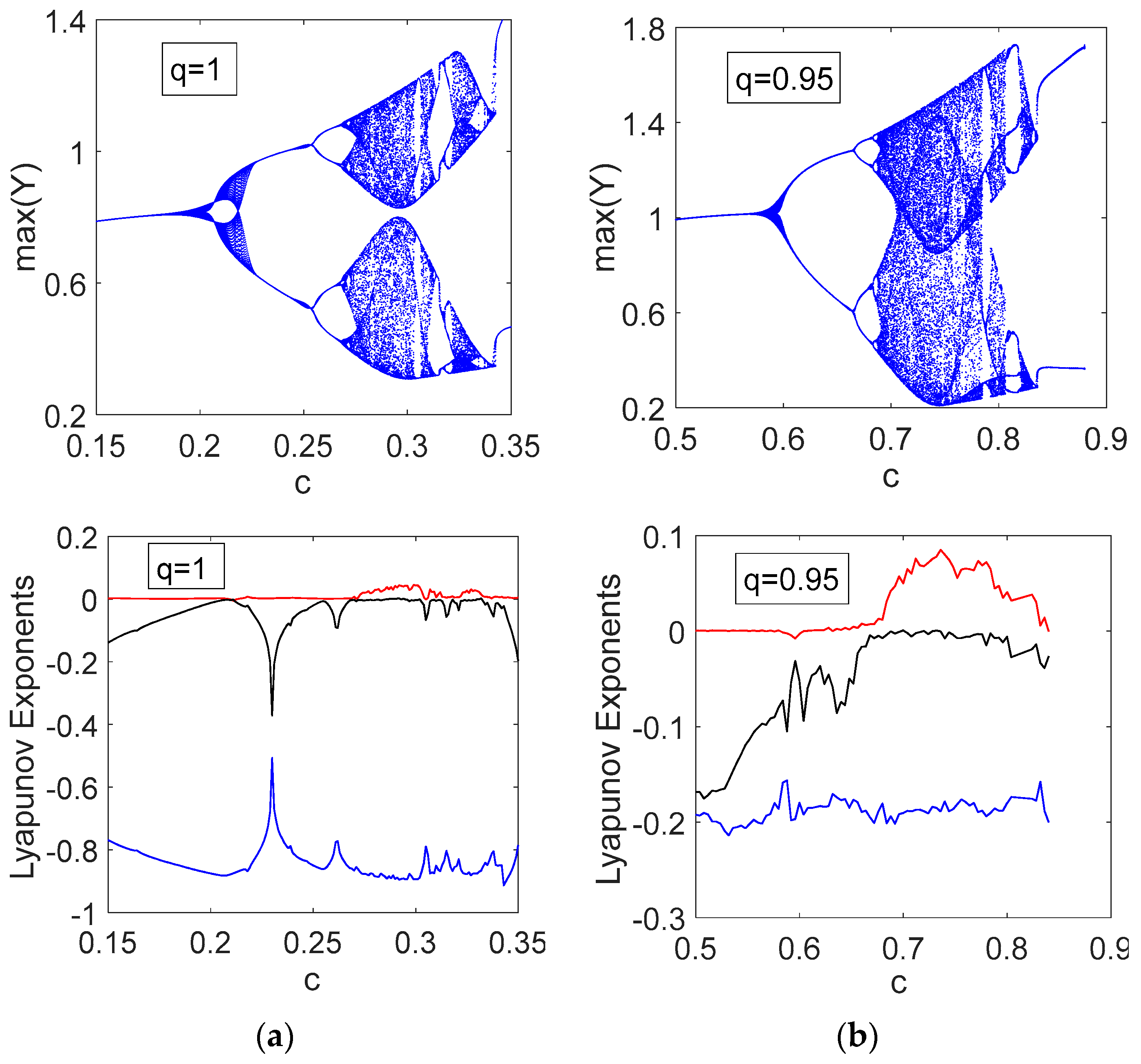
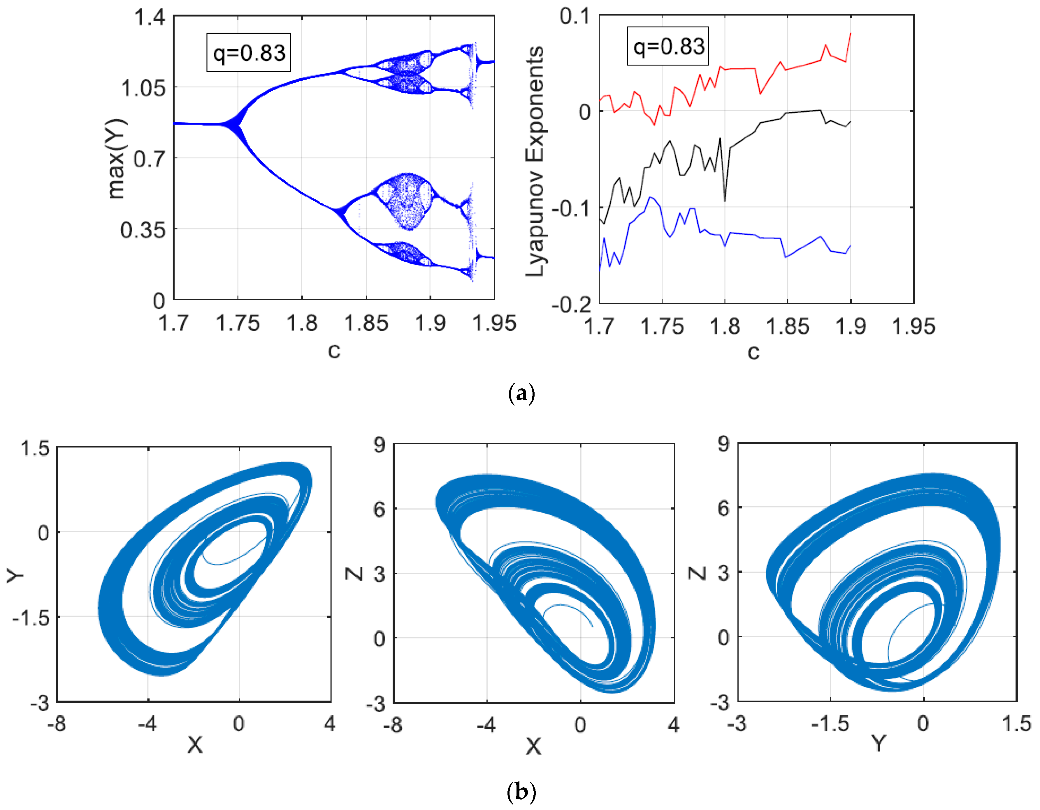
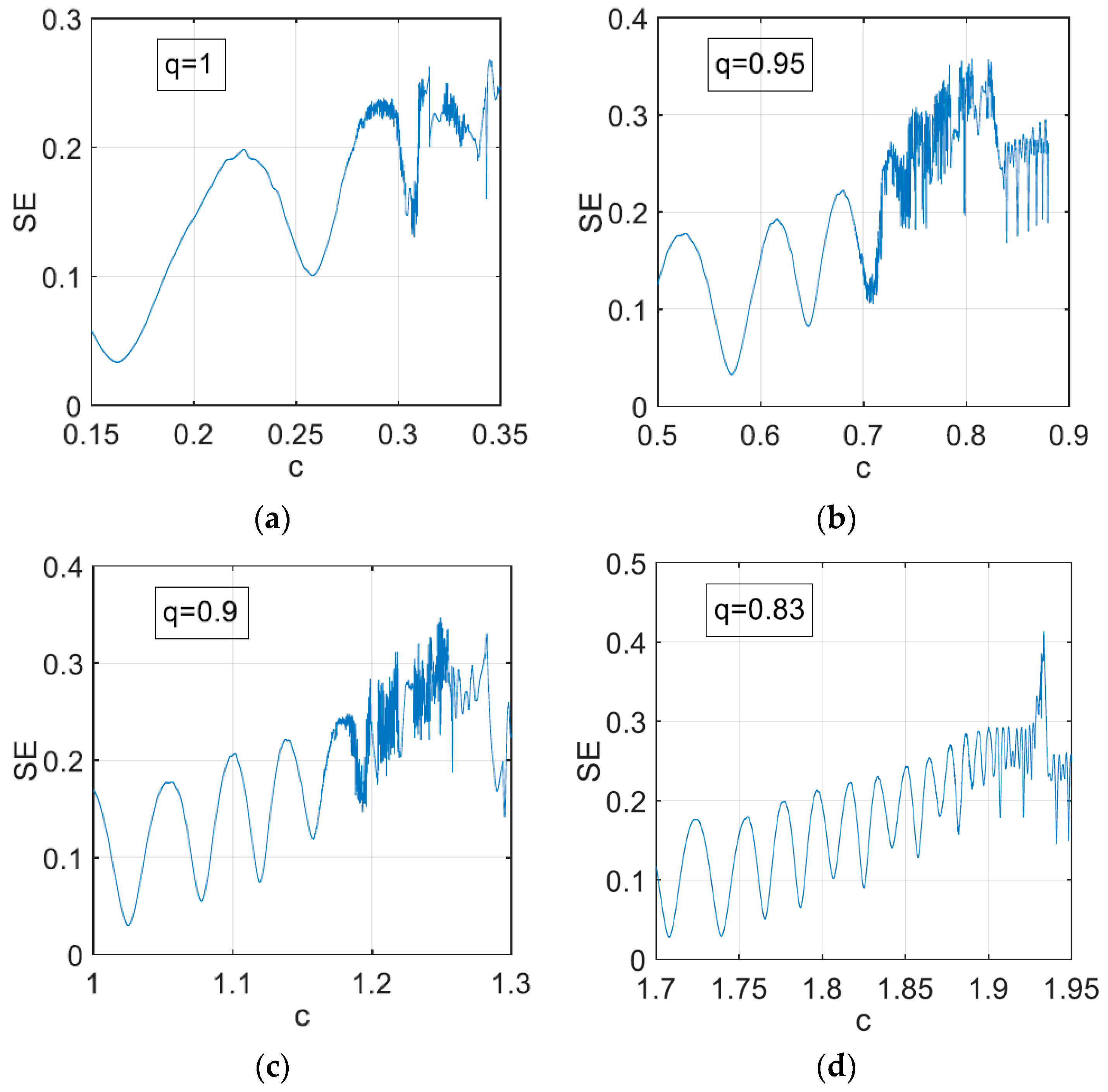
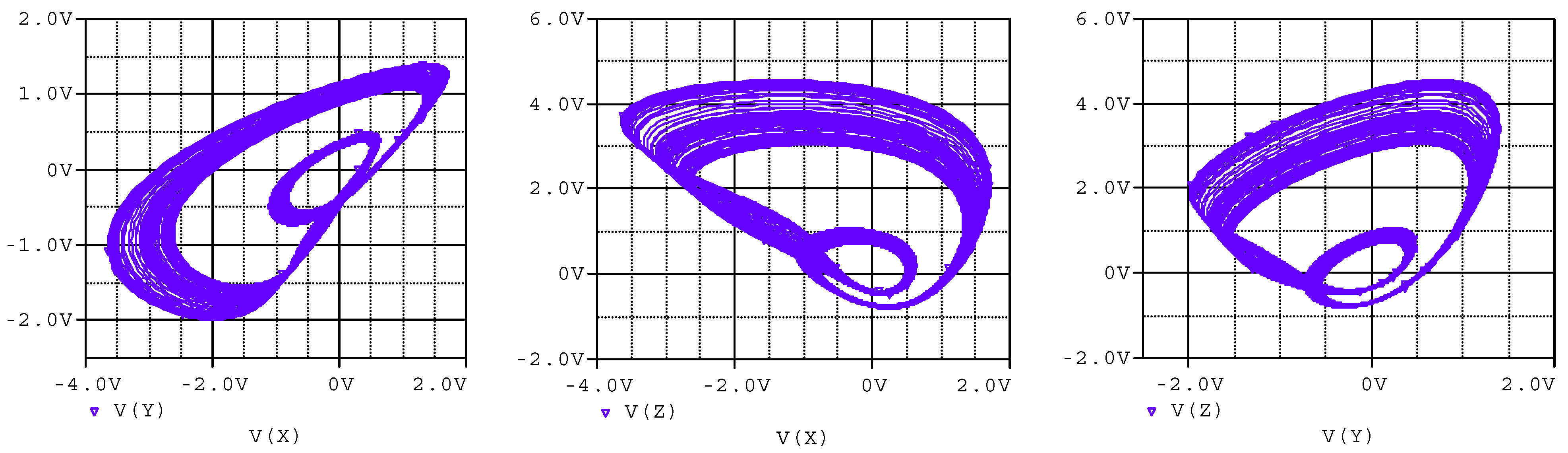
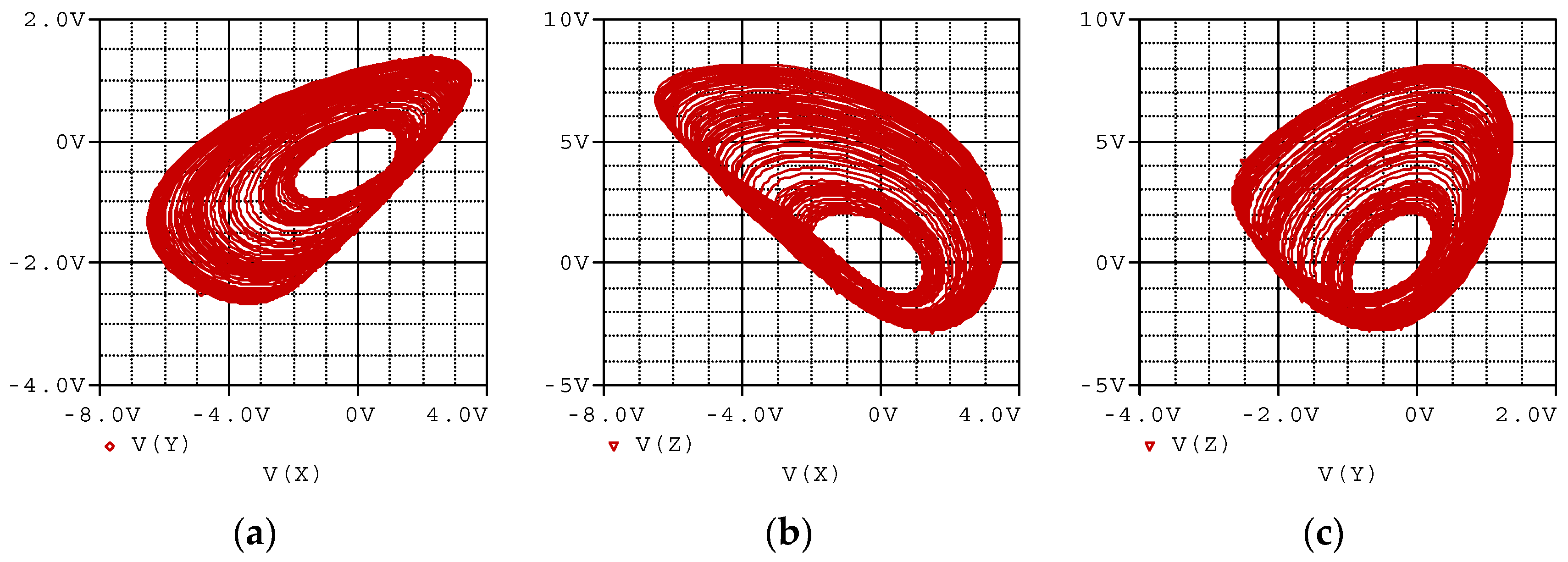
3. Dynamical Analyses of the Fractional-Order Sprott K System

It is difficult to solve a nonlinear fractional-order system analytically. Therefore, various methods have been developed to solve such systems. These methods include the use of Matlab-based tools such as fde12 [36], FOMCON [37] and ninteger [38]. In this study, the fde12 toolbox is utilized for performing all numerical analyses and simulations. To observe the chaotic behaviour and dynamical properties of the fractional-order Sprott K system, its spectra of Lyapunov exponents, SE complexity, Poincaré maps, and bifurcation diagrams are investigated in this section. Figure 1 depicts the bifurcation diagrams and Lyapunov spectra for both integer-order and fractional-order forms of the Sprott K system (2) with initial conditions x(0) = 0.5, y(0) = 0.5, and z(0) = 0.5. The parameter values a and b are set to 1 and 1 for the integer-order case, and to 1 and 2.3 for the fractional-order case. Figure 2 also illustrates the 2D chaotic phase portraits of the systems based on the corresponding bifurcation diagrams in Figure 1a,b.

After many simulations for various fractional-order values of q, it was observed that the output values of state variable z exceeded the limitations required to implement the electronic circuit. Thus, the system needs to be linearly scaled. The state variables are rescaled as x = v_x/V, y = v_y/V, and z = 2v_z/V. Accordingly, if the parameters are rearranged for q = 0.9, a and b should equal 2 and 1.75, respectively. Similarly, a = 2 and b = 2.55 can be chosen for q = 0.83. The parameter a is used as a linear scaling factor for both fractional-order q values. By using fde12 [39], Figure 3 and Figure 4 show the bifurcation diagrams, Lyapunov spectra, and 2D phase portraits versus various fractional-order values of q, respectively.

The results obtained from the calculations of Lyapunov exponents for fractional-order chaotic systems may not be highly accurate. Especially when the fractional degree q value is less than 0.9, it becomes difficult to calculate these exponents with the selected tools. Partially consistent Lyapunov exponent values can be obtained after conducting numerous simulations with different Schmid coefficient values [39,40]. In Figure 3 and Figure 4, the approximate Lyapunov exponential values are mostly similar to the corresponding bifurcation diagrams.

The detailed bifurcation diagram and the 2D phase portraits of the system (9) are presented in Figure 5a and Figure 5b, respectively. As shown in Figure 5b, when the parameter c is increased from 1.7 to 1.88, period-1, 2, 4, and 8 states as well as chaotic motion phase portraits can be observed. The period-doubling bifurcation route to chaos in Figure 5b illustrates the dynamic diversity of the system (9) for q = 0.83.

For a given N samples of time series, Spectral Entropy (SE) reflects the complexity of the dynamic behaviour [41]. In this complexity analysis method, flatter and reduced values of entropy indicate predictable dynamics, while higher and more variable values of entropy denote higher complexity [42]. In the present work, the calculating of SE begins by subtracting its average component as follows:

$$x(n)=x(n)-\overline{x}$$

(10)

where x(n) = {x(0), x(1), x … x(N − 1)} is N-sample time series and x represents the mean value of the series. Afterwards, the Discrete Fourier Transfer (DFT) of x(n) is computed as follows:

$$x(k)={\displaystyle \sum _{n=0}^{N-1}x(n)e^{-j\frac{2\pi nk}{N}}}$$

(11)

where k = 0, 1, … N − 1. With the calculated DFT, the relative power spectral density of X(k) is calculated as follows:

$$P(k)=\frac{{\left|X(k)\right|}^2}{{\displaystyle {\sum }_{k=0}^{\frac{N}{2}-1}{\left|X(k)\right|}^2}}$$

(12)

Lastly, SE is determined as follows:

$$SE=\frac{{\displaystyle {\sum }_{k=0}^{\frac{N}{2}-1}{\left|P_k\ln (P_k)\right|}^2}}{\ln (N/2)}$$

(13)

As can be seen from Figure 6, which shows the SE values as a function of the parameter c, the entropy values are in good agreement with the corresponding bifurcation diagrams. Particularly, when q is ‘1′, the system for c ∈ [0.27–0.34] shows higher and more variable values, which reflect chaotic behaviour. When q = 0.95, similar to the corresponding bifurcation diagram, the highest and most unstable entropy values are obtained when the system parameter c is between 0.7 and 0.83. Since q is 0.9, it is evident from Figure 6c that a dynamical change can be observed around c ∈ [1.17–1.24]. Lastly, when the value of c is around 1.89, the entropy values are high, consistent with the corresponding bifurcation diagrams. Thus, SE complexity analysis helps determine the chaotic behaviour for the selected values of q and c.

The Poincaré maps of the fractional-order Sprott K system for q = 0.83 and c = 1.88 in the planes are depicted in Figure 7. The presence of chaotic behaviour is evident in the distinct sets of points observed in the Poincaré map.

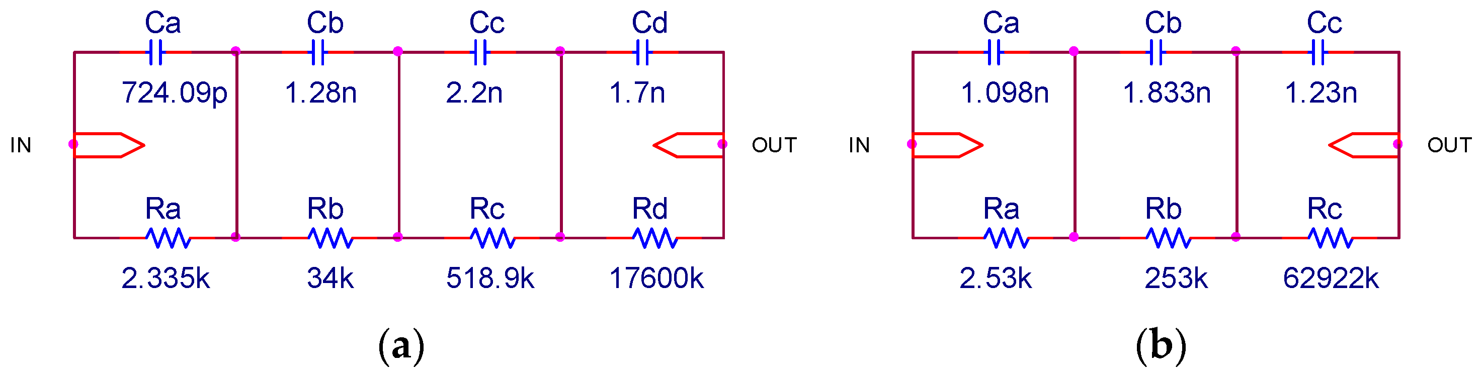
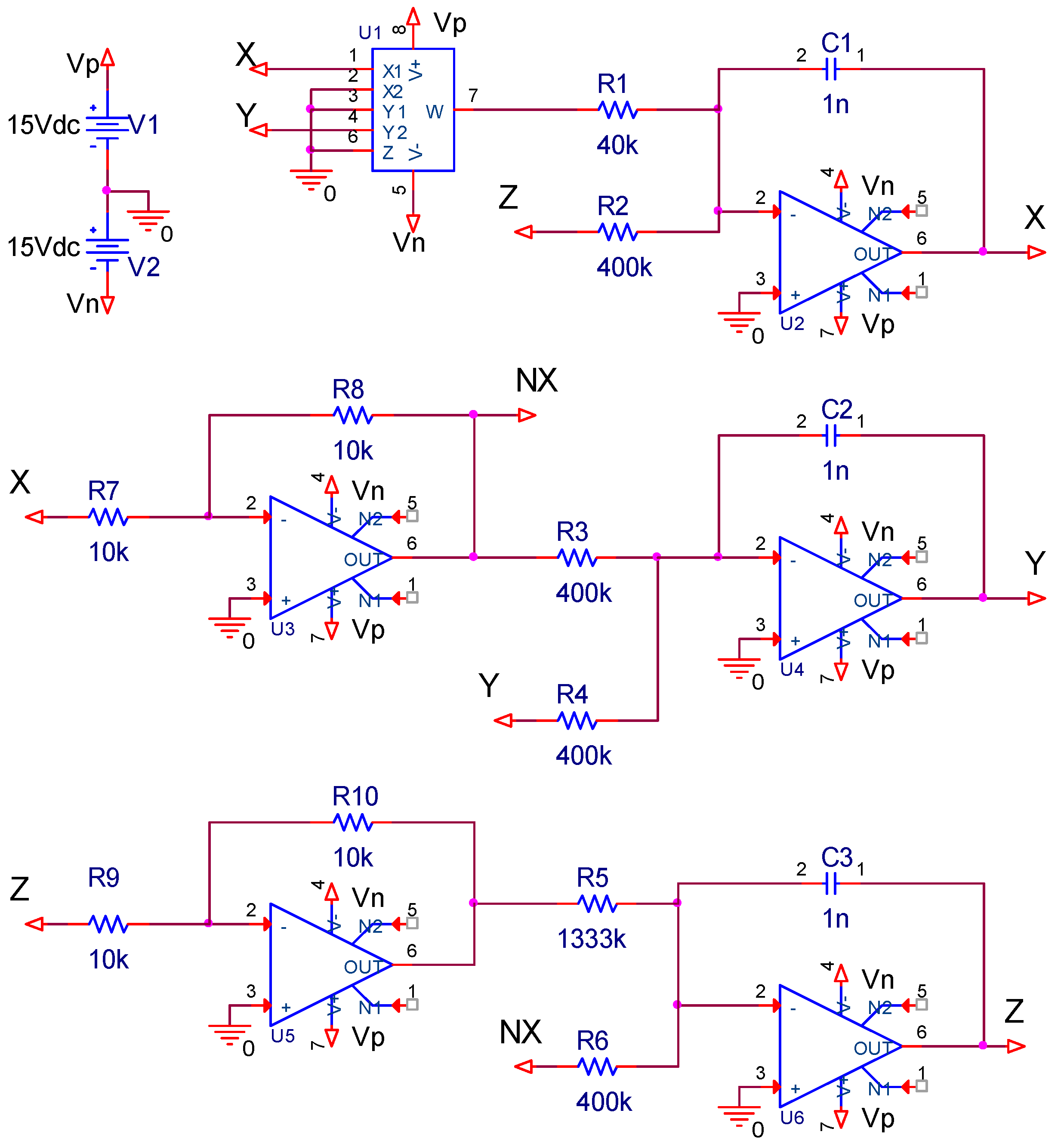
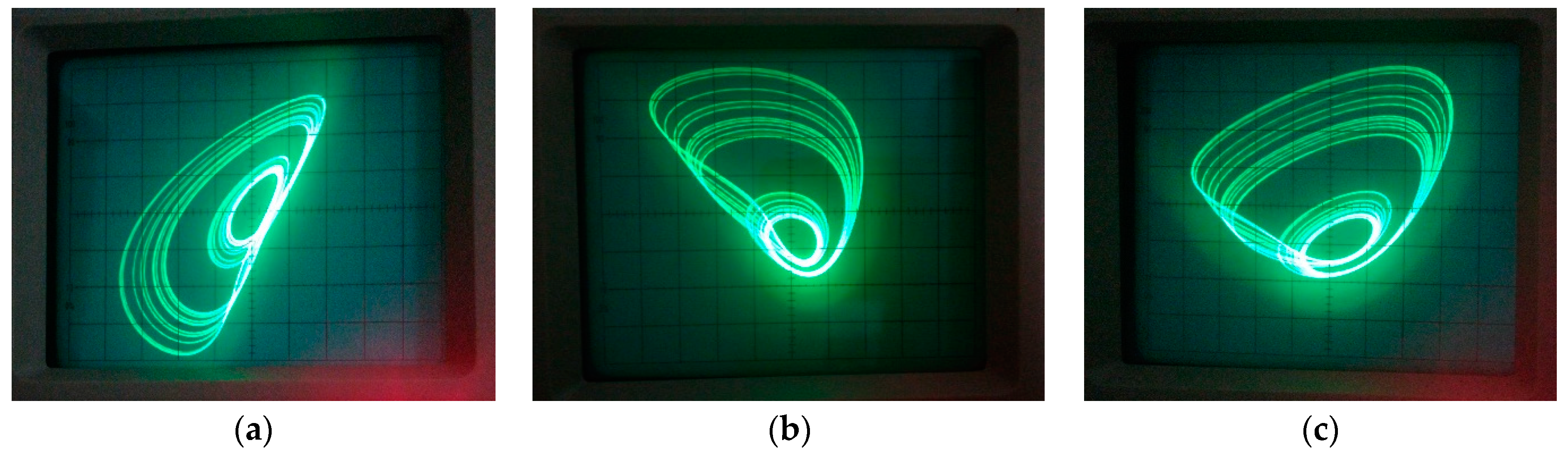
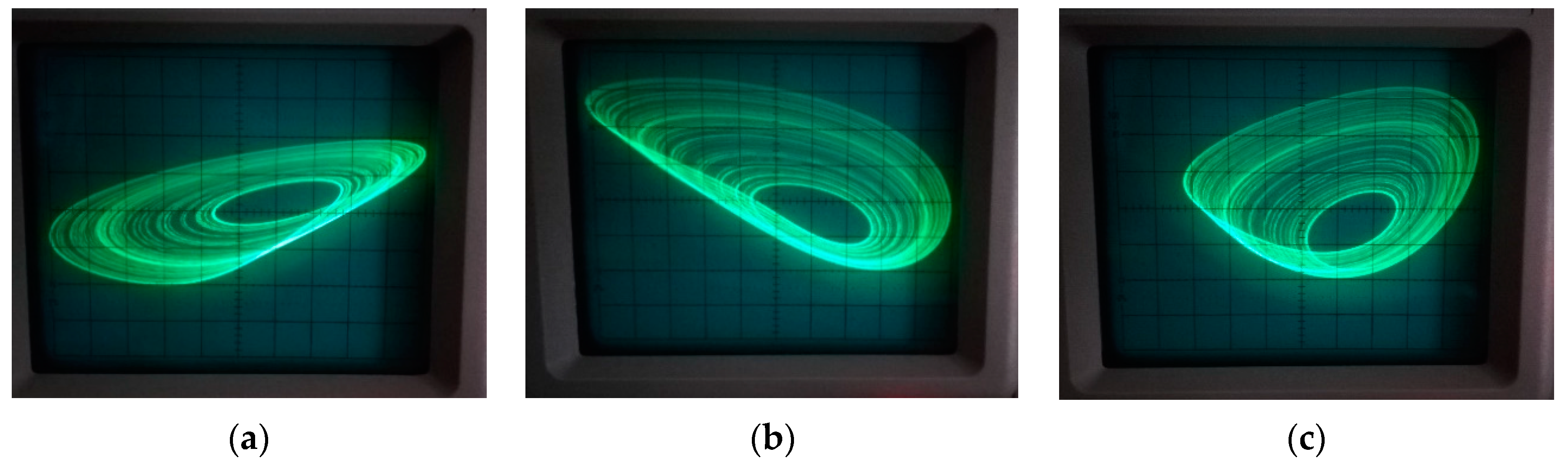
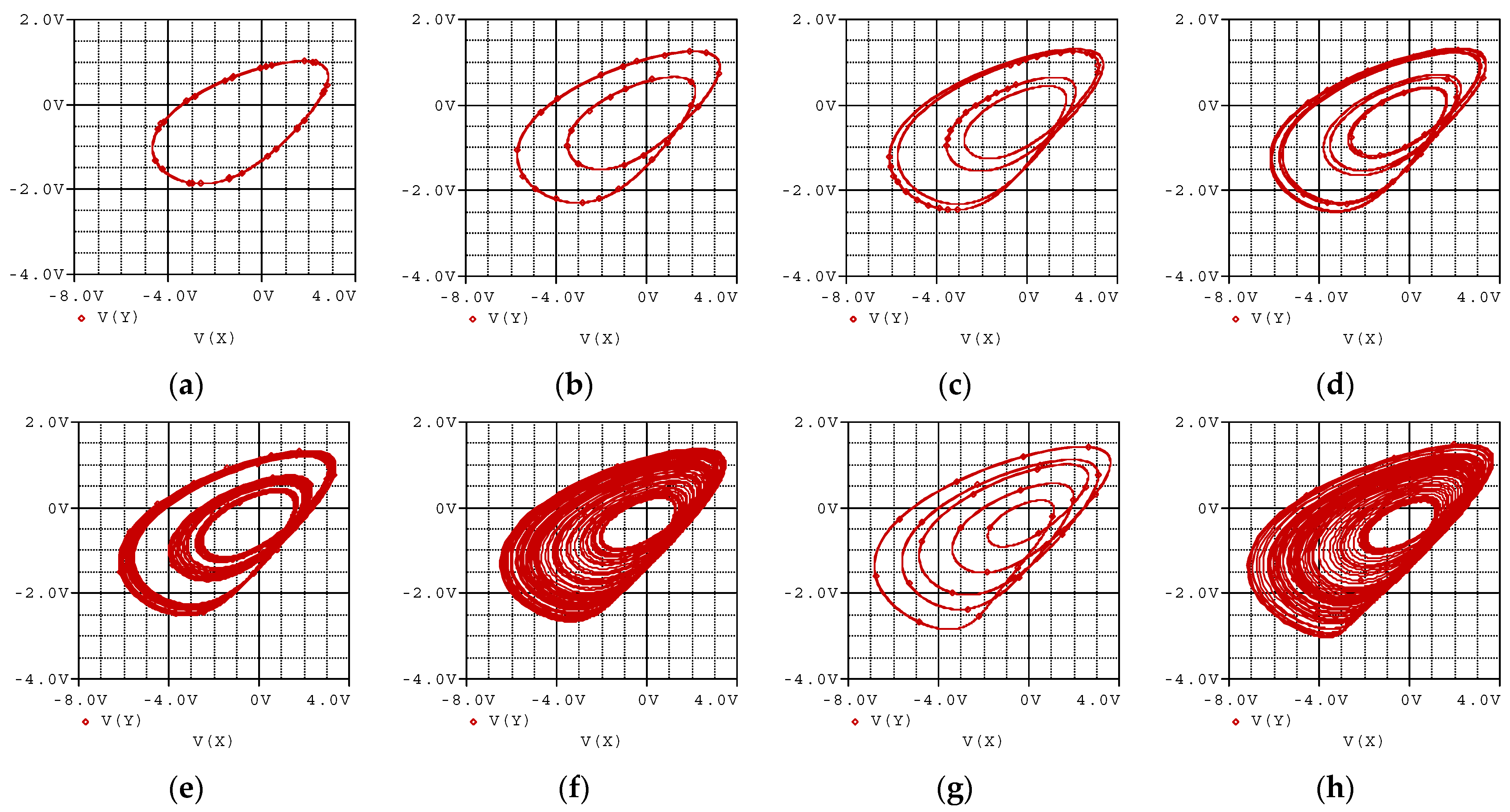
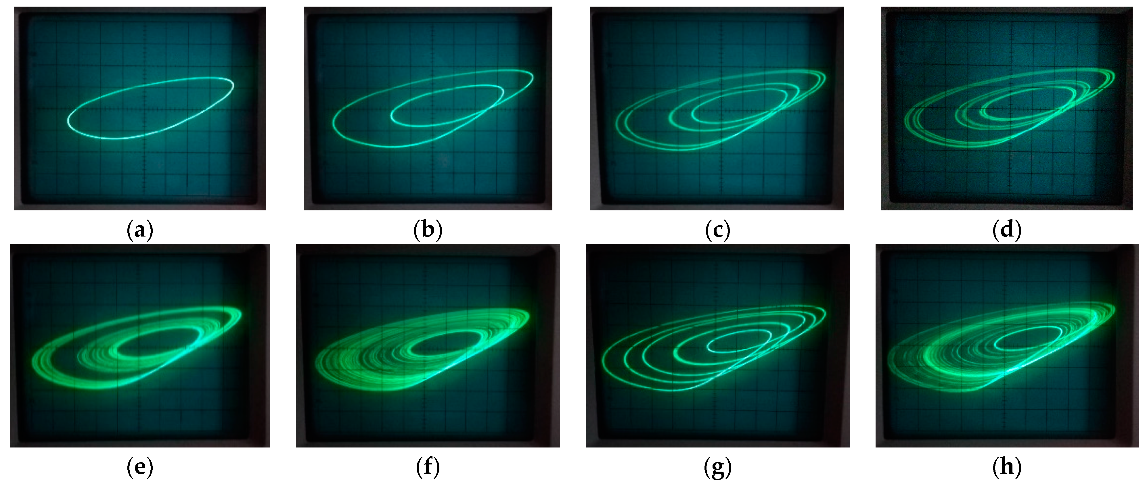
4. Electronic Circuit Realization of the Fractional-Order Sprott K Chaotic System

In this section, the realization of the fractional-order electronic circuit of the Sprott K oscillator, which was previously analyzed dynamically in the previous section, is presented for q = 0.83. Firstly, the implementation of the integer-order Sprott K system is described. Secondly, the realization of the fractional-order Sprott K system is presented for the lowest possible fractional-order value, and the boundaries at which the fractional-order system transitions between chaotic and periodic states are defined. For this purpose, the resistance and capacitance values of the module to be used in the fractional circuit of the system are determined. Finally, the application and simulation results are compared.

According to circuit theory, an electronic circuit exhibiting non-integer order dynamics is called a fractance [43]. Unlike integer-order systems, realizing electronic circuits for fractional-order systems requires specific resistor-capacitor (RC) circuits with fractal characteristics. Such a circuit is composed of topologically similar layers, depending on the approximate transfer function of a fractional-order system. Furthermore, the number of poles and zeros in the transfer function demonstrates the number of layers consisting of resistors and capacitors. There are three general approaches frequently used in the literature for fractance circuits, namely RC domino ladder, RC binary tree, and chain. In this study, the chain fractance approach, which includes N number serial RC pairs, is chosen. The chain fractance’s transfer function in the Laplace domain is written as follows according to the two-port network theory [2,16]:

$$H^{RC}(s)=\frac{1}{C_{1}s+\frac{1}{R_1}}+\frac{1}{C_{2}s+\frac{1}{R_2}}+\dots +\frac{1}{C_{N}s+\frac{1}{R_N}}$$

(14)

Using Equation (14), the following equations are obtained:

$$\frac{1}{s^{0.9}}\approx \frac{2.2675(s+1.29)(s+215.4)}{(s+0.0129)(s+2.154)(s+359.4)}$$

(15)

$$\frac{1}{s^{0.83}}\approx \frac{3.1869(s+135.5)(s+5.18)(s+0.1986)}{(s+235.9)(s+9.022)(s+0.3579)(s+0.000911)}$$

(16)

Taking into account Equations (15) and (16), the resistance and capacitance values of the fractional-order modules are presented in

Table 1. The resistance and capacitance values for fractional-order modules.

	q = 0.83	q = 0.9
Ra	2.335 kΩ	2.53 kΩ
Rb	34 kΩ	253 kΩ
Rc	518.9 kΩ	62.922 MΩ
Rd	17.6 MΩ
Ca	724.09 pF	1.0984 nF
Cb	1.28 nF	1.833 nF
Cc	2.2 nF	1.23 nF
Cd	1.7 nF

.

Based on Table 1, the circuit schematics of fractional-order modules can be seen in Figure 8.

The integer-order Sprott K system’s electronic circuit schematic is depicted in Figure 9. Since the output voltages fall within acceptable limits, linear scale operation is not required, and a = 1 and b = 1 are chosen. The control parameter and the initial conditions of the integer-order system are also selected as c = 0.3, x(0) = 0.5, y(0) = 0.5, and z(0) = 0.5, respectively.

Considering Figure 9, the dimensionless equations of the original Sprott K system are as follows:

$$\begin{array}{l}R{C}_1\frac{d{v}_x}{dt}=\frac{R{v}_x{v}_y}{10R_1}-\frac{R{v}_z}{R_2},\\ R{C}_2\frac{d{v}_y}{dt}=\frac{R{v}_x}{R_3}-\frac{R{v}_y}{R_4},\\ R{C}_3\frac{d{v}_z}{dt}=\frac{R{v}_z}{R_5}+\frac{R{v}_x}{R_6},\end{array}$$

(17)

where the component values are C_1,2,3 = 1 nF, R₁ = 40 kΩ, R_2,3,4,6 = 400 kΩ, R₅ = 1.33 MΩ, R_7,8,9,10 = 10 kΩ. The time scale factor RC and DC voltage sources are chosen as 0.4 ms, and V_P = −V_N = 15 V, respectively. Figure 10 shows the voltages on the X, Y, and Z terminals plotted against each other.

The electronic circuit of the integer-order Sprott K system with discrete elements is constructed on a board to compare it with the PSpice simulation. The phase portraits of the integer-order oscillator obtained from the circuit closely resemble the PSpice simulation results, as shown in Figure 11.

Modeling a fractional-order system with standard components is the major challenge of electronic circuit implementation. Here, circuits are constructed based on the parameter values obtained from the numerical analyses in the previous section. The fractional-order Sprott K circuit for q = 0.9, using the chain structure, is shown in Figure 12. The fractional integral operator $1/s^{0.9}$ is converted into a chain fractance of N = 3, with constant parameters of a = 2, b = 1.75, and c = 1.26. The initial conditions of the system are x(0) = 0.5, y(0) = 0.5, and z(0) = 0.5. As mentioned in the previous section, the state variables of the fractional-order circuit are re-scaled as x = v_x/V, y = v_y/V, and z = 2v_z/V for oscilloscope output views to be within an acceptable range, unlike the integer-order circuit schematic.

The electronic circuit shown in Figure 12 has the following component values: C_1,4,7 = 1.098 nF, C_2,5,8 = 1.833 nF, C_3,6,9 = 1.23 nF, R₁ = 40 kΩ, R₂ = 200 kΩ, R_3,4 = 400 kΩ, R₅ = 317.4 kΩ, R₆ = 228.57 kΩ, R_7,8,9,10 = 10 kΩ, R_11,14,17 = 2.53 kΩ, R_12,15,18 = 253 kΩ, R_13,16,19 = 62.922 MΩ. The time scale factor RC and DC voltage sources are chosen as 1 ms, and V_P = −V_N = 15 V, respectively. Figure 13 displays the voltages on the X, Y, and Z terminals plotted against each other.

The state variables of the fractional-order circuit for q = 0.83 are re-scaled as x = v_x/V, y = v_y/V, and z = 2v_z/V to ensure acceptable oscilloscope output limits. Considering Equation (9) and the re-scaling process, the values of the parameters are chosen to be approximately a = 2, b = 2.56, and c = 1.77 for electronic circuit implementation. The fractional-order Sprott K circuit for q = 0.83, using the chain structure, is depicted in Figure 14. Here, the fractional integral operator $1/s^{0.83}$ is converted into a chain fractance of N = 4. The initial conditions of the system are selected as x(0) = 0.5, y(0) = 0.5, and z(0) = 0.5. The circuits shown in Figure 9, Figure 12, and Figure 14 are composed of passive circuit elements with specified values, operational amplifiers (TL081), and multipliers (AD633) that can be easily found in the market as discrete circuit elements.

The component values of the electronic circuit in Figure 14 are as follows: C_1,5,9 = 724.09 pF, C_2,6,10 = 1.28 nF, C_3,7,11 = 2.2 nF, C_4,8,12 = 1.7 nF, R₁ = 40 kΩ, R₂ = 200 kΩ, R_3,4 = 400 kΩ, R₅ = 225 kΩ, R₆ = 156.24 kΩ, R_7,8,9,10 = 10 kΩ, R_11,15,19 = 2.335 kΩ, R_12,16,20 = 34 kΩ, R_13,17,21 = 518.9 kΩ, R_14,18,22 = 17.6 MΩ. The time scale factor RC and DC voltage sources are chosen as 0.4 ms, and V_P = −V_N = 18 V, respectively. Figure 15 depicts the voltages on the X, Y, and Z terminals versus each other. Additionally, FFT analysis results in the PSpice program are illustrated in Figure 16.

Moreover, to observe the real-time operating performance, the fractional-order Sprott K oscillator for q = 0.83 is implemented using discrete circuit elements. The oscilloscope views of the fractional-order oscillator are presented in Figure 17, which shows that the experimental results are in a good agreement with the simulation results, as expected.

Figure 18 and Figure 19 demonstrate the 2D phase planes of the fractional-order Sprott K oscillator in PSpice simulation and oscilloscope output views of circuit realization, respectively. In Figs. 16a-d, the period-doubling bifurcation route is shown as the system transitions from period-1 to period-2, 4, and 8 states, respectively, as the resistance value R₅ decreases from 232 to 216.8 kΩ. It can be observed that if the resistance value decreases further, the system exhibits chaotic behaviour. Due to the parasitic resistance effect of the active element circuits, there is a slight discrepancy in the control resistance values between the PSpice simulation outputs and the oscilloscope views of circuit realization. Additionally, robust chaos is obtained by reducing the R₅ resistance in the PSpice simulation and circuit implementation, which implies an increase in the c value in the numerical analysis. However, when the c value exceeds a certain threshold in numerical analysis, it is observed that the fde12 toolbox is insufficient in calculations, and some robust chaotic conditions cannot be obtained. Based on Figure 4, Figure 15, and Figure 17, it can be observed that the phase portraits of numerical analysis, PSpice simulation, and circuit implementation are similar. Furthermore, a period-doubling bifurcation route to chaotic behaviour is obtained in all three applications for fractional-order q values of 1, 0.9, and 0.83, respectively.

Contrary to prior research in the literature, it is observed that the electronic implementation of the Sprott K chaotic attractor exhibits chaotic behaviour for a low value of q, such as 0.83. Finally, Figure 20 illustrates the electronic circuit and fractional-order module of the fractional-order Sprott K oscillator for q = 0.83.

5. Conclusions

The diversity of a chaotic system’s dynamics can be enriched through fractional-order analysis. This study presents electronic circuit realizations of the Sprott K chaotic system with low-value fractional orders using standard components. The dynamic characteristic of the fractional-order system is investigated through numerical analyses, including time series, phase portraits, Lyapunov exponents, SE complexity, and bifurcation diagram calculations. The system exhibits rich dynamical behaviours, such as the period-doubling bifurcation route to chaos, thanks to fractional-order analysis. The bifurcation diagram analysis reveals that the system demonstrates chaotic motion for the fractional-order value of q = 0.83. Based on the presented bifurcation diagrams, the electronic circuit implementation of the Sprott K chaotic system is realized with a low-value fractional-order module. Additionally, the system’s PSpice schematic is simulated, and the simulation results are compared to analogue oscilloscope outputs of its electronic circuit realization, which uses standard components. The oscilloscope views of the electronic circuit confirm the simulation and numerical analysis results. Since the analogue realization of chaotic circuits with low-value fractional orders, such as non-integer order parameter q = 0.83, has not been reported in the literature, this study introduces a novel approach for calculating fractional-order chaotic systems. The Sprott K system is a simple six-term system; therefore, it is cost-effective. However, the fact that it can exhibit chaotic behaviour at different fractional degrees with the addition of extra coefficients increases its dynamic diversity and complexity. Considering the rich dynamics, cost-effectiveness, and complexity of the fractional-order Sprott K system, it is recommended for utilization in various analogue or digital engineering applications, such as synchronization, secure communication, and image encryption, where complexity, dynamic diversity, and applicability are of great importance.

References

1. Yang, F.; Wang, X. Dynamic characteristic of a new fractional-order chaotic system based on the Hopfield Neural Network and its digital circuit implementation. Phys. Scr. 2021, 96, 035218. [Google Scholar] [CrossRef]
2. Ahmad, W.M.; Sprott, J. Chaos in fractional-order autonomous nonlinear systems. Chaos Solitons Fractals 2003, 16, 339–351. [Google Scholar] [CrossRef] [Green Version]
3. Peng, Z.; Yu, W.; Wang, J.; Wang, J.; Chen, Y.; He, X.; Jiang, D. Dynamic analysis of seven-dimensional fractional-order chaotic system and its application in encrypted communication. J. Ambient. Intell. Humaniz. Comput. 2020, 11, 5399–5417. [Google Scholar] [CrossRef]
4. Zhang, Y.; Zhou, T. Three schemes to synchronize chaotic Fractional-order Rucklidge systems. Int. J. Mod. Phys. B 2007, 21, 2033–2044. [Google Scholar] [CrossRef]
5. Trikha, P.; Jahanzaib, L.S.; Nasreen; Baleanu, D. Dynamical analysis and triple compound combination anti-synchronization of novel fractional chaotic system. J. Vib. Control. 2021, 28, 1057–1073. [Google Scholar] [CrossRef]
6. Guang-Chao, Z.; Chong-Xin, L.; Yan, W. Dynamic analysis and finite time synchronization of a fractional-order chaotic system with hidden attractors. Acta Phys. Sin. 2018, 67, 050502. [Google Scholar] [CrossRef]
7. Akgul, A.; Adiyaman, Y.; Gokyildirim, A.; Aricioglu, B.; Pala, M.A.; Cimen, M.E. Electronic Circuit Implementations of a Fractional-Order Chaotic System and Observing the Escape from Chaos. J. Circuits Syst. Comput. 2022, 32, 2350085. [Google Scholar] [CrossRef]
8. Wang, J.; Xiao, L.; Rajagopal, K.; Akgul, A.; Cicek, S.; Aricioglu, B. Fractional-Order Analysis of Modified Chua’s Circuit System with the Smooth Degree of 3 and Its Microcontroller-Based Implementation with Analog Circuit Design. Symmetry 2021, 13, 340. [Google Scholar] [CrossRef]
9. Chen, D.; Liu, C.; Wu, C.; Liu, Y.; Ma, X.; You, Y. A New Fractional-Order Chaotic System and Its Synchronization with Circuit Simulation. Circuits Syst. Signal Process. 2012, 31, 1599–1613. [Google Scholar] [CrossRef]
10. Wang, M.; Liao, X.; Deng, Y.; Li, Z.; Su, Y.; Zeng, Y. Dynamics, synchronization and circuit implementation of a simple fractional-order chaotic system with hidden attractors. Chaos Solitons Fractals 2019, 130, 109406. [Google Scholar] [CrossRef]
11. Xiang-Rong, C.; Chong-Xin, L.; Fa-Qiang, W. Circuit realization of the fractional-order unified chaotic system. Chin. Phys. B 2008, 17, 1664–1669. [Google Scholar] [CrossRef]
12. Li, X.; Li, Z.; Wen, Z. One-to-four-wing hyperchaotic fractional-order system and its circuit realization. Circuit World 2020, 46, 107–115. [Google Scholar] [CrossRef]
13. Gokyildirim, A.; Calgan, H.; Demirtas, M. Fractional-Order sliding mode control of a 4D memristive chaotic system. J. Vib. Control. 2023. [Google Scholar] [CrossRef]
14. Liu, T.; Yan, H.; Banerjee, S.; Mou, J. A fractional-order chaotic system with hidden attractor and self-excited attractor and its DSP implementation. Chaos Solitons Fractals 2021, 145, 110791. [Google Scholar] [CrossRef]
15. Chen, D.; Wu, C.; Iu, H.H.C.; Ma, X. Circuit simulation for synchronization of a fractional-order and integer-order chaotic system. Nonlinear Dyn. 2013, 73, 1671–1686. [Google Scholar] [CrossRef]
16. Yao, J.; Wang, K.; Huang, P.; Chen, L.; Machado, J.T. Analysis and implementation of fractional-order chaotic system with standard components. J. Adv. Res. 2020, 25, 97–109. [Google Scholar] [CrossRef]
17. Rajagopal, K.; Nazarimehr, F.; Guessas, L.; Karthikeyan, A.; Srinivasan, A.; Jafari, S. Analysis, Control and FPGA Implementation of a Fractional-Order Modified Shinriki Circuit. J. Circuits Syst. Comput. 2019, 28, 1950232. [Google Scholar] [CrossRef]
18. Pham, V.-T.; Kingni, S.T.; Volos, C.; Jafari, S.; Kapitaniak, T. A simple three-dimensional fractional-order chaotic system without equilibrium: Dynamics, circuitry implementation, chaos control and synchronization. AEU Int. J. Electron. Commun. 2017, 78, 220–227. [Google Scholar] [CrossRef]
19. Hammouch, Z.; Mekkaoui, T. Circuit design and simulation for the fractional-order chaotic behavior in a new dynamical system. Complex Intell. Syst. 2018, 4, 251–260. [Google Scholar] [CrossRef]
20. Altun, K. FPAA Implementations of Fractional-Order Chaotic Systems. J. Circuits Syst. Comput. 2021, 30, 1–23. [Google Scholar] [CrossRef]
21. Altun, K. Kesir Dereceli Sprott-K Kaotik Sisteminin Dinamik Analizi ve FPGA Uygulaması. Eur. J. Sci. Technol. 2021, 25, 392–399. [Google Scholar] [CrossRef]
22. Dang, H.G. Dynamics and Synchronization of the Fractional-Order Sprott E System. Adv. Mater. Res. 2013, 850–851, 876–879. [Google Scholar] [CrossRef]
23. Dang, H.G. Adaptive Synchronization of the Fractional-Order Sprott N System. Adv. Mater. Res. 2013, 850–851, 872–875. [Google Scholar] [CrossRef]
24. Sprott, J.C. Some simple chaotic flows. Phys. Rev. E 1994, 50, R647–R650. [Google Scholar] [CrossRef] [PubMed]
25. Altun, K. Multi-Scroll Attractors with Hyperchaotic Behavior Using Fractional-Order Systems. J. Circuits Syst. Comput. 2021, 31, 22500852. [Google Scholar] [CrossRef]
26. Lu, J.G.; Chen, G. A note on the fractional-order Chen system. Chaos Solitons Fractals 2006, 27, 685–688. [Google Scholar] [CrossRef]
27. Pandey, A.; Baghel, R.K.; Singh, R.P. Analysis and circuit realization of a new autonomous chaotic system. Int. J. Electron. Commun. Eng. 2012, 5, 487–495. [Google Scholar]
28. Silva-Juárez, A.; Tlelo-Cuautle, E.; de la Fraga, L.G.; Li, R. FPAA-based implementation of fractional-order chaotic oscillators using first-order active filter blocks. J. Adv. Res. 2020, 25, 77–85. [Google Scholar] [CrossRef] [PubMed]
29. Du, M.; Wang, Z.; Hu, H. Measuring memory with the order of fractional derivative. Sci. Rep. 2013, 3, 3431. [Google Scholar] [CrossRef] [PubMed] [Green Version]
30. Ilten, E.; Demirtas, M. Fractional order super-twisting sliding mode observer for sensorless control of induction motor. COMPEL—Int. J. Comput. Math. Electr. Electron. Eng. 2019, 38, 878–892. [Google Scholar] [CrossRef]
31. Ozdemir, N.; Avci, D.; Iskender, B.B. The Numerical Solutions of a Two-Dimensional Space-Time Riesz-Caputo Fractional Diffusion Equation. Int. J. Optim. Control. Theor. Appl. IJOCTA 2011, 1, 17–26. [Google Scholar] [CrossRef]
32. Calgan, H.; Demirtas, M. A robust LQR-FOPIλDµ controller design for output voltage regulation of stand-alone self-excited induction generator. Electr. Power Syst. Res. 2021, 196, 107175. [Google Scholar] [CrossRef]
33. Yang, N.; Liu, C. A novel fractional-order hyperchaotic system stabilization via fractional sliding-mode control. Nonlinear Dyn. 2013, 74, 721–732. [Google Scholar] [CrossRef]
34. Demirtas, M.; Ilten, E.; Calgan, H. Pareto-based multi-objective optimization for fractional order PI^λ speed control of induction motor by using Elman neural network. Arab J. Sci. Eng. 2019, 44, 2165–2175. [Google Scholar] [CrossRef]
35. Ilten, E.; Demirtas, M. Off-Line Tuning of Fractional Order PIλ. J. Control. Eng. Appl. Inform. 2016, 18, 20–27. [Google Scholar]
36. Garrappa, R. Numerical Solution of Fractional Differential Equations: A Survey and a Software Tutorial. Mathematics 2018, 6, 16. [Google Scholar] [CrossRef] [Green Version]
37. Tepljakov, A. FOMCON: Fractional-Order Modeling and Control Toolbox. Fractional-Order Model. In Fractional-Order Modeling and Control of Dynamic Systems; Springer: Berlin/Heidelberg, Germany, 2017; pp. 107–129. [Google Scholar] [CrossRef]
38. Valério, D.; Sá da Costa, J. Ninteger: A non-integer control toolbox for MatLab. In Proceedings of the First IFAC Workshop on Fractional Differentiation and Applications, Bordeaux, France, 19–21 July 2004; pp. 208–213. [Google Scholar]
39. Danca, M.-F.; Kuznetsov, N. Matlab Code for Lyapunov Exponents of Fractional-Order Systems. Int. J. Bifurc. Chaos 2018, 28, 1850067. [Google Scholar] [CrossRef] [Green Version]
40. Wolf, A.; Swift, J.B.; Swinney, H.L.; Vastano, J.A. Determining Lyapunov exponents from a time series. Phys. D Nonlinear Phenom. 1985, 16, 285–317. [Google Scholar] [CrossRef] [Green Version]
41. He, S.; Sun, K.; Wang, H. Complexity Analysis and DSP Implementation of the Fractional-Order Lorenz Hyperchaotic System. Entropy 2015, 17, 8299–8311. [Google Scholar] [CrossRef] [Green Version]
42. Xiong, P.-Y.; Jahanshahi, H.; Alcaraz, R.; Chu, Y.-M.; Gómez-Aguilar, J.; Alsaadi, F.E. Spectral Entropy Analysis and Synchronization of a Multi-Stable Fractional-Order Chaotic System using a Novel Neural Network-Based Chattering-Free Sliding Mode Technique. Chaos Solitons Fractals 2021, 144, 110576. [Google Scholar] [CrossRef]
43. Podlubny, I. Fractional Differential Equations, Mathematics in Science and Engineering; Academic Press: New York, NY, USA, 1999. [Google Scholar]
Figure 1. Integer-order and fractional-order Sprott K systems’ bifurcation diagrams and Lyapunov exponents (red, black, and blue lines represent λ1, λ2, and λ3, respectively) for different parameter values: (a) q = 1, a = 1, b = 1, (b) q = 0.95, a = 1, b = 2.3.
Fractalfract 07 00470 g001
Figure 2. 2D chaotic phase portraits of systems (2) and (9) for t(s) [0, 1000]: (a) q = 1, a = 1, b = 1, c = 0.3, (b) q = 0.95, a = 1, b = 2.3, c = 0.75.
Fractalfract 07 00470 g002
Figure 3. Dynamical analyses of Sprott K system for q = 0.9, a = 2, b = 1.75, and x(0) = 0.5, y(0) = 0.5, z(0) = 0.5: (a) the corresponding bifurcation diagram and Lyapunov exponents (red, black, and blue lines represent λ1, λ2, and λ3, respectively), (b) chaotic phase portraits for c = 1.24.
Fractalfract 07 00470 g003
Figure 4. Dynamical analyses of system (9) for q = 0.83, a = 2, b = 2.55, and x(0) = 0.5, y(0) = 0.5, z(0) = 0.5: (a) the corresponding bifurcation diagram and Lyapunov exponents (red, black, and blue lines represent λ1, λ2, and λ3, respectively), (b) 2D phase portraits for c = 1.88.
Fractalfract 07 00470 g004
Figure 5. The corresponding detailed bifurcation diagram and x-y phase portraits for the fractional-order Sprott K system with q = 0.83: (a) The bifurcation diagram of the local maximum of y, and (b) period-doubling bifurcation route to chaos for c [1.7–1.88] and t(s) [200, 500].
Fractalfract 07 00470 g005
Figure 6. SE complexity analyses for (a) q = 1, (b) q = 0.95, (c) q = 0.9, and (d) q = 0.83.
Fractalfract 07 00470 g006
Figure 7. The Poincaré maps of the fractional-order Sprott K system (q = 0.83 and c = 1.88).
Fractalfract 07 00470 g007
Figure 8. The fractional-order integrators’ circuit schematic in the PSpice program: (a) q = 0.83, (b) q = 0.9.
Fractalfract 07 00470 g008
Figure 9. Electronic circuit schematic of the Sprott K system.
Fractalfract 07 00470 g009
Figure 10. Phase portraits of the system (12) in PSpice simulation.
Fractalfract 07 00470 g010
Figure 11. Oscilloscope views for R5 = 1.33 MΩ: (a) vx (1 V/div) versus vy (0.5 V/div), (b) vx (1 V/div) versus vz (1 V/div), (c) vy (0.5 V/div) versus vz (1 V/div).
Fractalfract 07 00470 g011
Figure 12. Electronic circuit schematic of the fractional-order Sprott K attractor for q = 0.9.
Fractalfract 07 00470 g012
Figure 13. Phase portraits of the fractional-order Sprott K system in PSpice simulation for q = 0.9, R5 = 317.4 kΩ (c = 1.26), t = 10 –100 ms and maximum step size = 10µs: (a) vx versus vy, (b) vx versus vz, (c) vy versus vz.
Fractalfract 07 00470 g013
Figure 14. Circuit schematic of the fractional-order Sprott K attractor for q = 0.83.
Fractalfract 07 00470 g014
Figure 15. Phase planes of the fractional-order Sprott K system in PSpice simulation for q = 0.83, R5 = 225 kΩ, t = 100–200 ms, and maximum step size = 10µs: (a) vx versus vy, (b) vx versus vz, (c) vy versus vz.
Fractalfract 07 00470 g015
Figure 16. Simulation results of FFT analyses in the PSpice program.
Fractalfract 07 00470 g016
Figure 17. Oscilloscope views for R5 = 215.3 kΩ: (a) vx (1 V/div) versus vy (1 V/div), (b) vx (1 V/div) versus vz (2 V/div), (c) vy (0.5 V/div) versus vz (2 V/div).
Fractalfract 07 00470 g017
Figure 18. Phase planes of the fractional-order Sprott K system in PSpice simulation for t = 100–200 ms and maximum step size = 10µs: (a) R5 = 245 kΩ, (b) R5 = 235 kΩ, (c) R5 = 230 kΩ, (d) R5 = 228.8 kΩ, (e) R5 = 228.25 kΩ, and (f) R5 = 225 kΩ, (g) R5 = 221 kΩ, (h) R5 = 218 kΩ.
Fractalfract 07 00470 g018
Figure 19. Oscilloscope views of vx (1 V/div) versus vy (1 V/div) for various R5 values (a) R5 = 232 kΩ, (b) R5 = 220.7 kΩ, (c) R5 = 218.4 kΩ, (d) R5 = 216.8 kΩ, (e) R5 = 217.1 kΩ, and (f) R5 = 215.3 kΩ, (g) R5 = 212.2 kΩ, (h) R5 = 210.2 kΩ.
Fractalfract 07 00470 g019
Figure 20. Analog circuits for q = 0.83: (a) The fractional-order Sprott K oscillator, (b) the fractional-order module.
Fractalfract 07 00470 g020