Article

A Hybrid Local Radial Basis Function Method for the Numerical Modeling of Mixed Diffusion and Wave-Diffusion Equations of Fractional Order Using Caputo’s Derivatives

1
Department of Mathematics, Islamia College Peshawar, Peshawar 25120, Khyber Pakhtunkhwa, Pakistan
2
Mathematics Department, Al-Qunfudhah University College, Umm Al-Qura University, Al-Qunfudhah 28821, Saudi Arabia
*
Authors to whom correspondence should be addressed.
Fractal Fract. 2023, 7(5), 381; https://doi.org/10.3390/fractalfract7050381
Submission received: 8 April 2023 / Revised: 26 April 2023 / Accepted: 28 April 2023 / Published: 1 May 2023
(This article belongs to the Special Issue Advances in Fractional Modeling and Computation)

Abstract

:
This article presents an efficient method for the numerical modeling of time fractional mixed diffusion and wave-diffusion equations with two Caputo derivatives of order 0 < α < 1 , and 1 < β < 2 . The numerical method is based on the Laplace transform technique combined with local radial basis functions. The method consists of three main steps: (i) first, the Laplace transform is used to transform the given time fractional model into an equivalent time-independent inhomogeneous problem in the frequency domain; (ii) in the second step, the local radial basis functions method is utilized to obtain an approximate solution for the reduced problem; (iii) finally, the Stehfest method is employed to convert the obtained solution from the frequency domain back to the time domain. The use of the Laplace transform eliminates the need for classical time-stepping techniques, which often require very small time steps to achieve accuracy. Additionally, the application of local radial basis functions helps overcome issues related to ill-conditioning and sensitivity to shape parameters typically encountered in global radial basis function methods. To validate the efficiency and accuracy of the proposed method, several test problems in regular and irregular domains with uniform and non-uniform nodes are considered.

1. Introduction

Fractional order calculus (FOC) has not been explored in engineering and other sciences, due to its inherent complexity, as well as the fact that it lacks a completely valid geometric or physical interpretation [1]. However, some natural behaviors related to different fields of engineering are more accurately represented by using it; now, it is a promising tool used in physics [2], fluid mechanics [3], signal processing [4], thermal diffusion phenomenon [5], botanical electrical impedances [6], robotics [7], etc. Various analytical and numerical methods have been developed for fractional order differential equations (FODEs). For instance, in [8], the authors derived the analytic solution of the fractional diffusion wave equation using the Wright function. Liu et al. [9] obtained the complete solution of the time fractional advection–dispersion equation by employing Mellin and Laplace transforms as well as the properties of H functions. Mainardi [10] obtained the fundamental solution of the fractional diffusion-wave equation using an auxiliary function. Wyss [11] obtained the solution of the fractional diffusion equation using Fox functions. Some notable works have been done on the theoretical analysis of FODEs (see [12,13,14] and references therein).
Fractional partial differential equations (FPDEs) in mathematical models have experienced significant growth in recent years, establishing them as one of the most crucial topics in the field of fractional order calculus (FOC). Several FPDE-based models have been proposed [15,16,17], and various analytical and numerical schemes have been developed to solve them. Numerous authors have studied the numerical solution of FPDEs. For instance, Liu et al. [18] employed a first-order finite difference scheme for both time and space derivatives, deriving stability conditions in the process. Zhao et al. [19] used the finite element method to solve the multi-term time fractional mixed diffusion and diffusion-wave equation with a variable coefficient. In [20], an ADI spectral method based on the Legendre spectral approximation in space and finite difference method in time was developed to obtain the solution of wave-diffusion equations. Agrawal [21] obtained the general solution of wave-diffusion equations using the Laplace transform and finite sine transform. Tadjeran et al. [22] obtained the solution of the fractional diffusion equation using the Crank–Nicholson technique combined with the spatial extrapolation method. Li and Chen [23] employed three methods: finite difference methods, Galerkin finite element methods, and spectral methods, for numerical simulations of FPDEs. Lie et al. [24] utilized the fully discrete spectral method to solve multi-term fractional mixed diffusion and diffusion wave equations. Dehgan et al. [25] applied the homotopy analysis method to study the numerical solutions of various nonlinear FPDEs.
Different types of meshless methods are rapidly gaining popularity due to their meshless nature and ease of implementation for multi-dimensional problems on a set of uniform or non-uniform nodes in regular and irregular domains. Numerous meshless methods have been developed for the numerical modeling of partial differential equations (PDEs). For instance, Liu et al. [26] proposed an implicit meshless approach based on radial basis functions for solving fractional diffusion equations. Chen et al. [27] solved the time fractional diffusion equation using the Kansa method. Shivanian and Jafarbadi [28] employed the spectral meshless radial point interpolation technique coupled with finite difference discretization for the numerical simulation of fractional diffusion equations. Meshless methods can be categorized into two types: global meshless methods (GMMs) and local meshless methods (LMMs). A GMM has two major disadvantages, namely a dense ill-conditioned interpolation matrix and sensitivity to shape parameters. To overcome these issues, the LMM was developed in [29].
In an LMM, collocation is performed over small overlapping domains of influence. This approach allows for solving small systems of linear equations, with dimensions equal to the number of nodes in each domain of influence, for each node individually. LMMs have found applications in various scientific and engineering problems. For instance, in [30], the authors proposed an efficient local meshless upwind method based on radial basis functions (RBFs) for the numerical simulation of the time fractional advection–diffusion equation. Kumar and Bhardwaj [31] developed a local meshless method for the numerical solution of the nonlinear time fractional diffusion wave equation. Bhardwaj and Kumar [32] introduced an efficient local RBF-based meshless method for the numerical simulation of Tricomi-type equations of fractional order. The authors of [33,34] obtained the numerical solutions of linear and nonlinear time fractional diffusion waves and the telegraph equation using local RBFs. Hosseini et al. [35] obtained the approximate solution of the time fractional diffusion wave equation with damping via an efficient meshless local radial point interpolation method. Salehi [36] used a meshless point collocation method to solve the multi-term fractional diffusion wave equation. An RBF-based meshless technique was proposed in [37] for the approximate solution of the time fractional diffusion-wave equation. Yang et al. [38] employed the moving least squares approximation method for the numerical approximation of fractional diffusion wave equations. Other works on the applications of RBF-based local meshless methods can be found in the references (see [39,40,41,42] and the references therein).
Many researchers have investigated the time fractional mixed diffusion and wave diffusion equation. Sun et al. [43] obtained the solution of the fractional mixed diffusion and wave diffusion equation using an L-type difference scheme. The authors of [19] proposed a linear triangle finite element method for the numerical simulation of the multi-term fractional mixed diffusion and wave diffusion equation. Feng et al. [44] obtained the solution of the 2D multi-term fractional mixed sub-diffusion and wave-diffusion equation using finite difference and finite element methods. Liu et al. [24] proposed an efficient fully discrete spectral method for the numerical modeling of the fractional mixed diffusion and diffusion wave equations. Bhardwaj and Kumar [45] obtained the numerical solution of the fractional mixed diffusion and wave diffusion equation using an efficient local RBF-based meshless method. The authors used the finite difference method for time discretization; for space discretization, an RBF-based local collocation method was used.
In this work, our aim is to approximate the solution of fractional mixed diffusion and wave diffusion equations using an RBF-based local meshless method coupled with Laplace transform. The RBF-based local meshless methods are easy to implement for solving problems in irregular and complex geometries and offer high accuracy at a low computational cost. Additionally, the Laplace transform is employed to overcome stability limitations associated with finite difference temporal discretization techniques. To the best of our knowledge, this is the first attempt to utilize the RBF-based local meshless method coupled with Laplace transform for the numerical modeling of time fractional mixed diffusion and wave diffusion problems. In this study, we consider a fractional mixed diffusion and wave diffusion problem of the following form:
0 c D t α u ( θ ¯ , t ) + 0 c D t β u ( θ ¯ , t ) = Δ u ( θ ¯ , t ) + f ( θ ¯ , t ) , ( θ ¯ , t ) Ω × [ 0 , T ] , u ( θ ¯ , 0 ) = ξ ( θ ¯ ) , u ( θ ¯ , 0 ) t = η ( θ ¯ ) , θ ¯ Ω , L b u ( θ ¯ , t ) = β ( θ ¯ , t ) , θ ¯ Ω ,
where 0 < α < 1 , 1 < β < 2 and ξ ( θ ¯ ) , η ( θ ¯ ) , and f ( θ ¯ , t ) are sufficiently smooth functions on domain Ω , with its boundary Ω , and the Caputo derivatives 0 c D t α u ( θ ¯ , t ) and 0 c D t β u ( θ ¯ , t ) of order α and β are defined by
0 c D t α u ( θ ¯ , t ) = 1 Γ ( 1 α ) 0 t u ( θ ¯ , τ ) τ ( t τ ) α d τ , 0 < α < 1 ,
and
0 c D t β u ( θ ¯ , t ) = 1 Γ ( 2 β ) 0 t 2 u ( θ ¯ , τ ) τ 2 ( t τ ) 1 β d τ , 1 < β < 2 .
The rest of the paper is organized as follows: Section 2.1 discusses the time discretization through Laplace transform. Section 2.2 discusses spatial discretization using the local RBF method. Section 2.3 explains the Stehfest method for the numerical inversion of the Laplace transform. Section 2.4 focuses on the error analysis of the method. Section 3 addresses the stability of the method. Section 4 presents numerical examples to demonstrate the effectiveness of the proposed method. Finally, Section 5 provides the conclusions.

2. Proposed Numerical Method

In our proposed numerical method, there are three main steps: (i) time discretization via the Laplace transform, (ii) spatial discretization via the local RBF method, and (iii) a numerical inversion of the Laplace transform via the Stehfest method.

2.1. (i) Time Discretization via the Laplace Transform

In this section, we use the Laplace transform to transform the problem into an equivalent time-independent problem and avoid the time stepping technique. The Laplace transform of a u ( θ ¯ , t ) is defined as
L u ( θ ¯ , t ) = u ^ ( θ ¯ , z ) = 0 e z t u ( θ ¯ , t ) d t ,
the Laplace transform of the Caputo derivative 0 c D t α u ( θ ¯ , t ) is defined as
L 0 c D t α u ( θ ¯ , t ) = z α u ^ ( θ ¯ , z ) z α 1 u ( θ ¯ , 0 ) ,
and the Laplace transform of the Caputo derivative 0 c D t β u ( θ ¯ , t ) is defined as
L 0 c D t β u ( θ ¯ , t ) = z β u ^ ( θ ¯ , z ) z β 1 u ( θ ¯ , 0 ) z β 2 u t ( θ ¯ , 0 ) .
Applying the Laplace transform to the model defined in (1), we have
L 0 c D t α u ( θ ¯ , t ) + 0 c D t β u ( θ ¯ , t ) = L Δ u ( θ ¯ , t ) + f ( θ ¯ , t ) ,
and
L L b u ( θ ¯ , t ) = L β ( θ ¯ , t ) ,
which implies
z α u ^ ( θ ¯ , z ) z α 1 u ( θ ¯ , 0 ) + z β u ^ ( θ ¯ , z ) z β 1 u ( θ ¯ , 0 ) z β 2 u t ( θ ¯ , 0 ) = Δ u ^ ( θ ¯ , z ) + f ^ ( θ ¯ , z ) ,
and
L b u ^ ( θ ¯ , z ) = β ( θ ¯ , z ) ,
simplifying the above equations, we obtain the following system
( z α I + z β I L g ) u ^ ( θ ¯ , z ) = F ^ ( θ ¯ , z ) ,
L b u ^ ( θ ¯ , z ) = β ( θ ¯ , z ) ,
where F ^ ( θ ¯ , z ) = z α 1 ξ ( θ ¯ ) + z β 1 ξ ( θ ¯ ) z β 2 η ( θ ¯ ) + f ^ ( θ ¯ , z ) and L g = Δ , where I denotes the identity operator, L g is the linear differential operator, and L b is the boundary differential operator. In order to obtain the solutions of the systems in (2) and (3), first, we use the local RBF method to discretize the operators L g and L b , then systems (2) and (3) are solved in parallel for each point z in the complex plane (see, e.g., [46]). Finally, the solution of the original problem (1) is obtained using the inverse Laplace transform. The local RBF method is described in the next section.

2.2. (ii) Spatial Discretization via Local RBF Method

In the local RBF method, the problem and its corresponding boundary are interpolated on n g nodes that can be distributed regularly or irregularly. For each node θ ¯ j ( j = 1 , 2 , 3 , , n g ) , there is a local domain Ω j = { θ ¯ i j } j = 1 n l ( i = 1 , 2 , 3 , , n g ) , where n l denotes the number of nodes in the local domain Ω j . Thus, the local RBF interpolant of u ^ ( θ ¯ ) is of the form,
u ^ ( θ ¯ j ) = i = 1 n l λ i j φ ( θ ¯ j θ ¯ i j ) ,
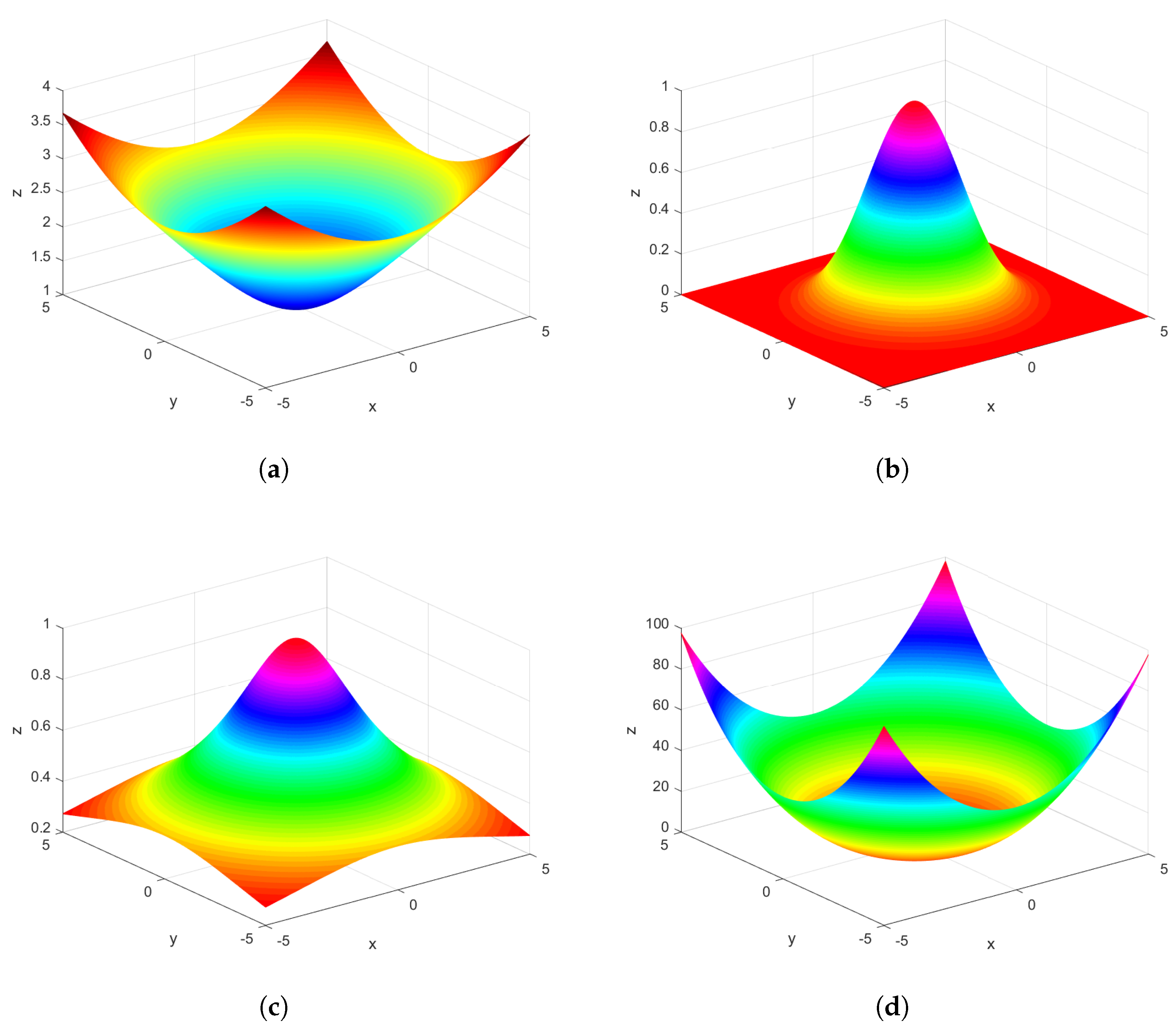
where the vector λ j = { λ i j } i = 1 n g is a vector of unknown expansion coefficients, φ ( r ) is a RBF and r = θ ¯ j θ ¯ i j denotes the distance between θ ¯ j and θ ¯ i j . In the literature, there are several RBFs. Some commonly used RBFs are listed in Table 1 and the corresponding graphs are shown in Figure 1.
In this study, we select MQ RBF and GA RBF, which are defined as
φ ( θ ¯ j θ ¯ i j ) = 1 + ε 2 θ ¯ j θ ¯ i j 2 ,
and
φ ( θ ¯ j θ ¯ i j ) = e x p ( ε 2 θ ¯ j θ ¯ i j 2 ) ,
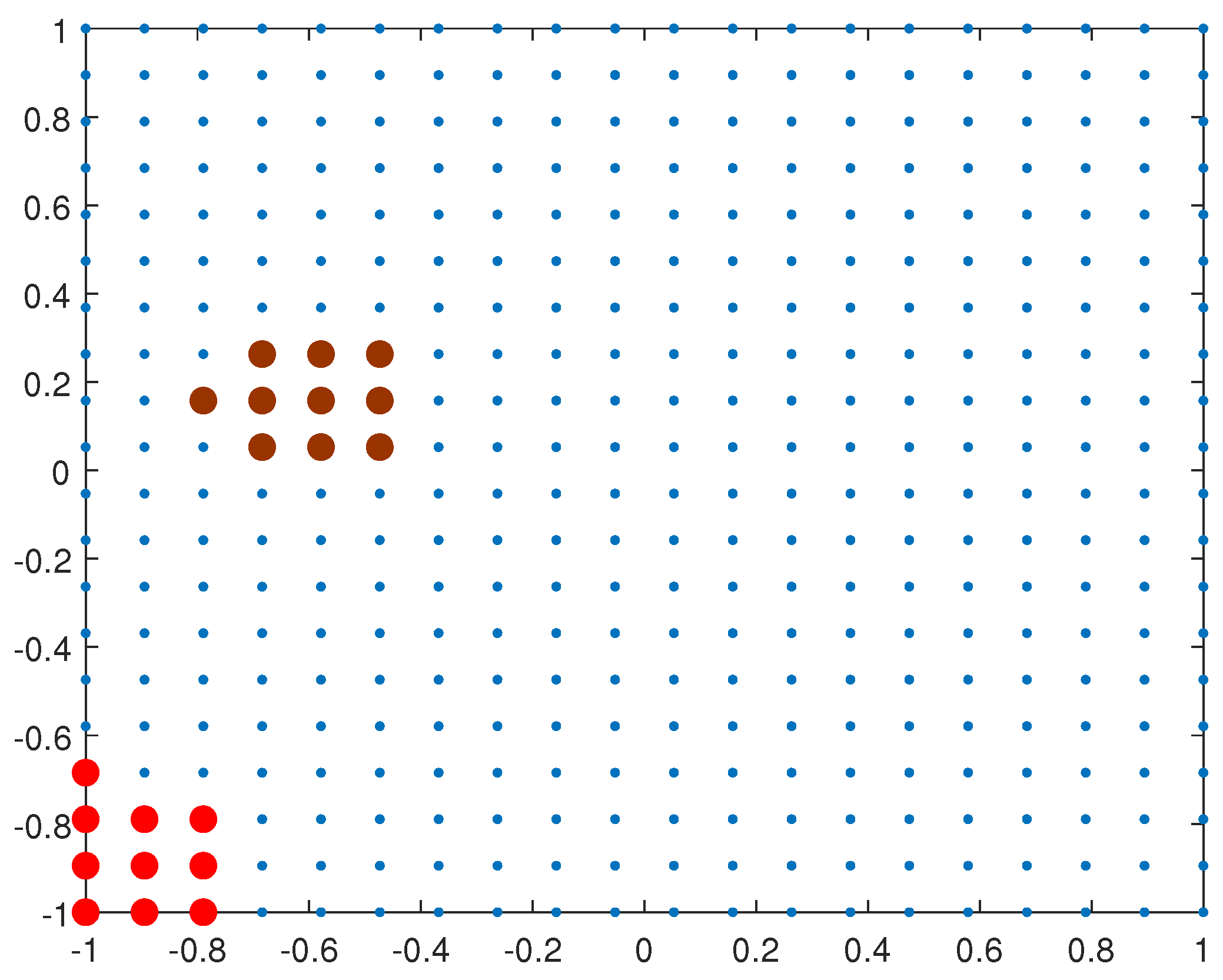
where ε denotes the shape parameter. Each node θ ¯ i j and its n l 1 neighbors are referred to as a stencil. A typical stencil is shown in Figure 2.
At each stencil, we obtain the n l × n l matrix, given as
u ^ j = B j λ j ,
where u ^ j = [ u ( θ ¯ 1 j ) , u ( θ ¯ 2 j ) , , u ( θ ¯ n l j ) ] T , B j = [ ϕ ( θ ¯ k j θ ¯ i j ) ] 1 k , i n l , and λ j = [ λ 1 j , λ 2 j , , λ n l j ] T . The invertibility of the system (5) requires the following definitions
Definition 1
[47]. A function ζ ( r ) is completely monotone on [ 0 , ) , if
1. 
ζ ( r ) C [ 0 , ) .
2. 
ζ ( r ) C [ 0 , ) .
3. 
( 1 ) m ζ ( m ) ( r ) 0 , for m = 1 , 2 , 3 ,
Theorem 1
[47]. If ζ ( r ) = φ ( r ) C [ 0 , ) and ζ ( r ) > 0 for r > 0 . Let ζ ( r ) be completely monotone and non-constant on ( 0 , ) , then for any set of n g distinct centers θ ¯ j ( j = 1 , 2 , 3 , , n g ) , the interpolation matrix B j is invertible.
The unknown coefficients λ j in Equation (5) can be computed as
λ j = ( B j ) 1 u ^ j ,
whose entries are
λ 1 j λ 2 j . . . λ n l j = φ ( θ ¯ 1 j θ ¯ 1 j ) φ ( θ ¯ 1 j θ ¯ 2 i ) . . . φ ( θ ¯ 1 j θ ¯ n l j ) φ ( θ ¯ 2 j θ ¯ 1 j ) φ ( θ ¯ 2 j θ ¯ 2 i ) . . . φ ( θ ¯ 2 j θ ¯ n l j ) . . . . . . . . . . . . . . . . . . φ ( θ ¯ n l j θ ¯ 1 j ) φ ( θ ¯ n l j θ ¯ 2 j ) . . . φ ( θ ¯ n l j θ ¯ n l j ) 1 u ^ ( θ ¯ 1 j ) u ^ ( θ ¯ 2 j ) . . . u ^ ( θ ¯ n l j ) .
The differential operator L g can be approximated as
L g u ^ = i = 1 n l λ i j L φ ( θ ¯ i θ ¯ i j ) ,
which can be written as
L g u ^ = ψ j ( B j ) 1 u ^ j ,
where ψ j = [ L ϕ ( θ ¯ k j θ ¯ i j ) ] 1 k , i n l . Hence, we have
L g u ^ = Ψ j u ^ j ,
where Ψ j = ψ j ( B j ) 1 . Equation (7), is the local form; the global form can be obtained by expanding Ψ j to Y by inserting zeros into each row in corresponding positions. Therefore, the approximation of the differential operator L at each θ ¯ j is given as
L g u ^ = Y u ^ .
The matrix Y is sparse, having n g n l zero entries and n l non-zero entries. The boundary differential operator L b can be approximated in a similar way
L b u ^ = Φ u ^ ,
using Equations (8) and (9) in Equations (2) and (3), we obtained the following fully discrete system
( z α I + z β I Y ) u ^ ( θ ¯ , z ) = F ^ ( θ ¯ , z ) ,
Φ u ^ ( θ ¯ , z ) = β ( θ ¯ , z ) .
Now, solving the system defined in Equations (10) and (11) for each point z in the complex plan will give us the solution u ^ ( θ ¯ , z ) .

Selection: Good Value of the Shape Parameter

We utilized MQ RBF and GA RBF in our numerical experiments. These RBFs contain parameter ε ; for optimal accuracy of the numerical solution, the value of ε varies. The condition number C d of the matrix B j is used to quantify the sensitivity to perturbation of the linear system. In this work, the uncertainty principle [48] is used for the best shape parameter ε .
The necessary steps for obtaining the optimal value of shape parameter ε are presented in the following Algorithm 1.
Algorithm 1: Optimal Shape Parameter
1:
Input:  C d m i n ,   C d m a x ,   ε I n c r e m e n t
2:
Step 1:  C d = 1  
3:
Step 2: select 10 + 12 < C d < 10 + 16  
4:
Step 3:  while   C d > C d m a x   and   C d < C d m i n  
5:
Step 4: Construct the matrix B j  
6:
Step 5:  E , S , P = s v d ( B j )  
7:
Step 6:  C d = ρ m a x ρ m i n  
8:
Step 7:  if   C d < C d m i n ,   ε = ε ε I n c r e m e n t  
9:
Step 8:  if   C d > C d m a x ,   ε = ε + ε I n c r e m e n t  
10:
Output:  ε ( optimal ) = ε .
After obtaining the best value of the shape parameter, we compute ( B j ) 1 using svd as ( B j ) 1 = ( ESP T ) 1 = PS 1 E T (see [49]). Hence, we can calculate Ψ j in (7).

2.3. (iii) Stehfest Method

In this section, we utilize the Stehfest algorithm for numerically inverting the Laplace transform. It is one of the most important algorithms used for the numerical inversion of the Laplace transform. This method was developed in the late 1960s [50,51]. Due to its simplicity and performance, it is becoming popular in many areas, such as economics, geophysics, financial mathematics, chemistry, and computational physics. This method is fast and gives good results for smooth functions. The solution u ( θ ¯ , t ) can be retrieved via the Stehfest method, as
u ( θ ¯ , t ) = l n 2 t i = 1 N ρ i u ^ ( θ ¯ , z ) ,
where the weights ρ i are given by
ρ i = ( 1 ) N 2 + i p = i + 1 2 m i n ( i , N 2 ) p N 2 ( 2 p ! ) ( N 2 p ) ! p ! ( p 1 ) ! ( i p ) ! ( 2 p i ) ! .
Here, N , refers to the Stehfest number, which should be even. Solving (10) and (11) for parameters z = l n 2 t i , i = 1 , 2 , 3 , , N in the LT space. Using (12), the original solution can be obtained.
The Gaver–Stehfest algorithm possesses several attractive properties. Firstly, the approximations of any function using this algorithm are linear in the values of the transform. Secondly, it only requires the values of the transform function for real z. Thirdly, the computation of the coefficients is straightforward. Lastly, the approximations obtained using this algorithm are exact for constant functions. The Gaver–Stehfest algorithm has been extensively studied by various authors, as documented in [52,53]. These studies have demonstrated that this method has very fast convergence for non-oscillatory functions.

2.4. Error Analysis

Here, we discuss the error analysis of the proposed method. In step (a), we employ the LT, which is analytic; thus, no error occurs in this step. The error of the method arises in steps (b) and (c). In step (b), we utilize the RBF-based local meshless method, which has an error estimate of order O ( σ 1 ε H d ) , 0 < σ < 1 , where H d denotes the fill distance and ε is the shape parameter [47]. In step (c), the Stehfest method is employed for the numerical inversion of the LT. The error analysis of this method has been studied in [54,55], where the authors conducted various numerical experiments to investigate the effects of the involved parameters on the accuracy and efficiency of the method. They noted that “If β significant digits are required, suppose N = 2.2 β positive integer. Set the precision of the system at ν = 1.1 N . Then for the argument t and u ^ ( θ ¯ , z ) , calculate u ( θ ¯ , t ) in (12).” According to these observations, the following error estimation is obtained.
Remark 1
[56]. If the error of input data satisfies 10 ( ν + 1 ) u ^ u u 10 ν , where N is a positive even integer via ν = 1.1 N , then the error is 10 ( β + 1 ) u ^ u u 10 β , where N = 1.1 β .

3. Stability

Here, we discuss the stability of the fully discrete systems (10) and (11). We express the system in the following form
C u ^ = R ,
the coefficient matrix C is obtained using the local meshless method. The constant for the stability of the system (14) is defined as
δ = sup u ^ 0 u ^ C u ^ ,
δ has a finite value for any norm . defined in R N . From Equation (15), we obtain
C 1 u ^ C u ^ δ .
Moreover, we can write
C = sup v 0 C v v .
where C is the pseudoinverse of C . Therefore,
C sup v = C u ^ 0 C C u ^ C u ^ = sup u ^ 0 u ^ C u ^ = δ .
Equations (16) and (17) give the bounds for the constant δ . For system (14), the pseudoinverse may be hard to compute, but by using it, stability is guaranteed. The MATLAB condest function can be used for evaluating C 1 as
δ = c o n d e s t ( C ) C

4. Applications

This section focuses on presenting numerical results and discussions. The performance, efficiency, accuracy, and convergence of the proposed method are tested and validated using five test problems in one and two dimensions. For two-dimensional problems, six different sets of regular and irregular domains with uniform and non-uniform points are selected. Three error norms are utilized: the maximum absolute error, the relative error, and the root mean square error, which are denoted and defined as follows:
E r r o r 1 = max 1 j n g | u ( ζ j , t ) u k ( ζ j , t ) | ,
E r r o r 2 = j = 1 n g ( u ( ζ ¯ j , t ) u k ( ζ ¯ j , t ) ) 2 n g ,
E r r o r 3 = j = 1 n g ( u ( ζ j , t ) u k ( ζ j , t ) ) 2 j = 1 n g ( u ( ζ j , t ) ) 2 ,
where n g represents the total number of points, n l represents the points in the sub-domain, and N represents the points used in the Stehfest method. u ( ζ j , t ) denotes the analytic solution, and u k ( ζ j , t ) denotes the numerical solution. The numerical experiments are conducted using MQ and GA RBFs. In all experiments, the initial conditions, boundary conditions, and source terms are calculated based on the analytic solutions. All of the numerical experiments are performed with a final time of T = 1 .
Problem 1.
Consider the following one-dimensional test problem
0 c D t α u ( x , t ) + 0 c D t β u ( x , t ) = Δ u ( x , t ) + f ( x , t ) , 0 x 1 ,
with the exact solution
u ( x , t ) = t 3 sin ( π x ) .
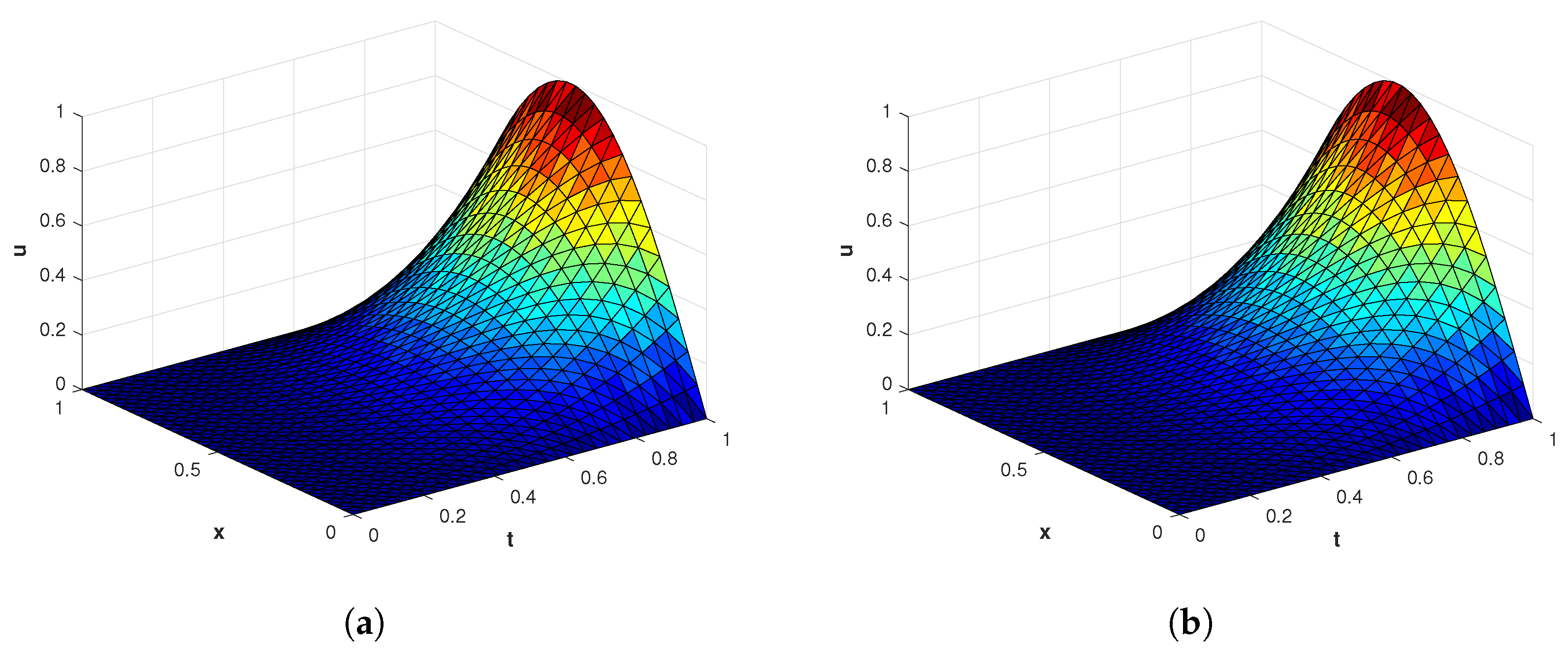
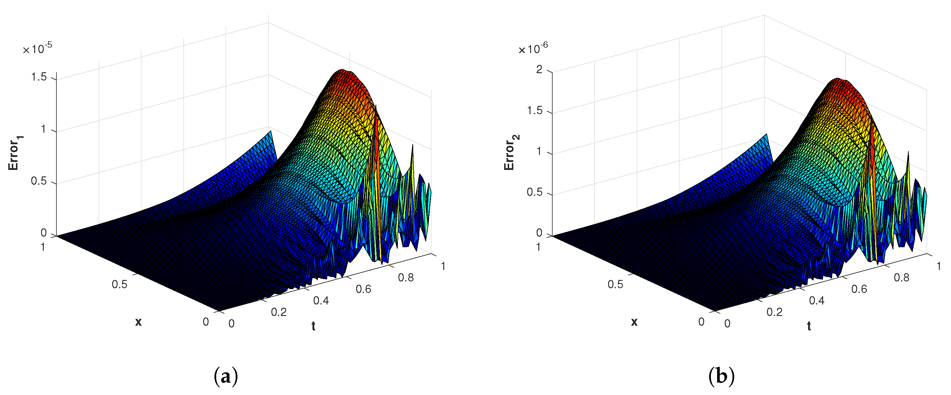
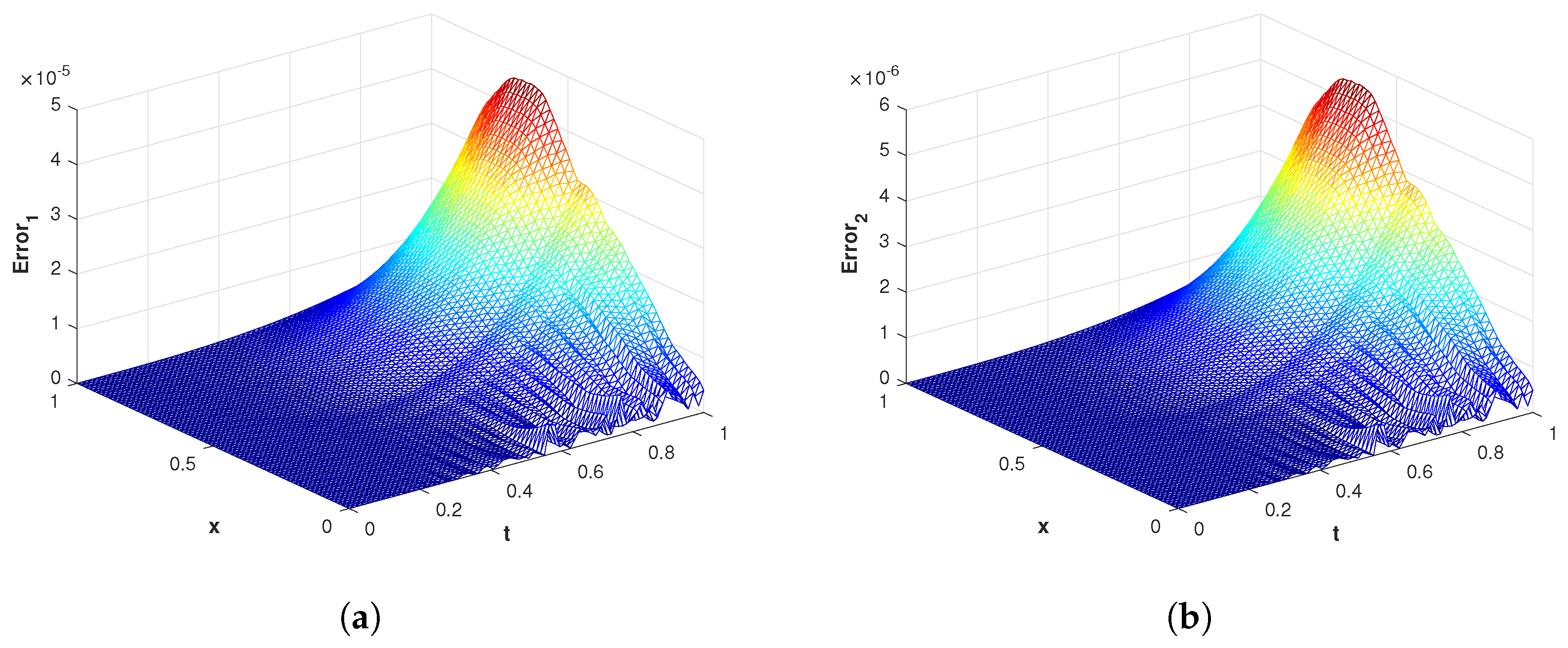
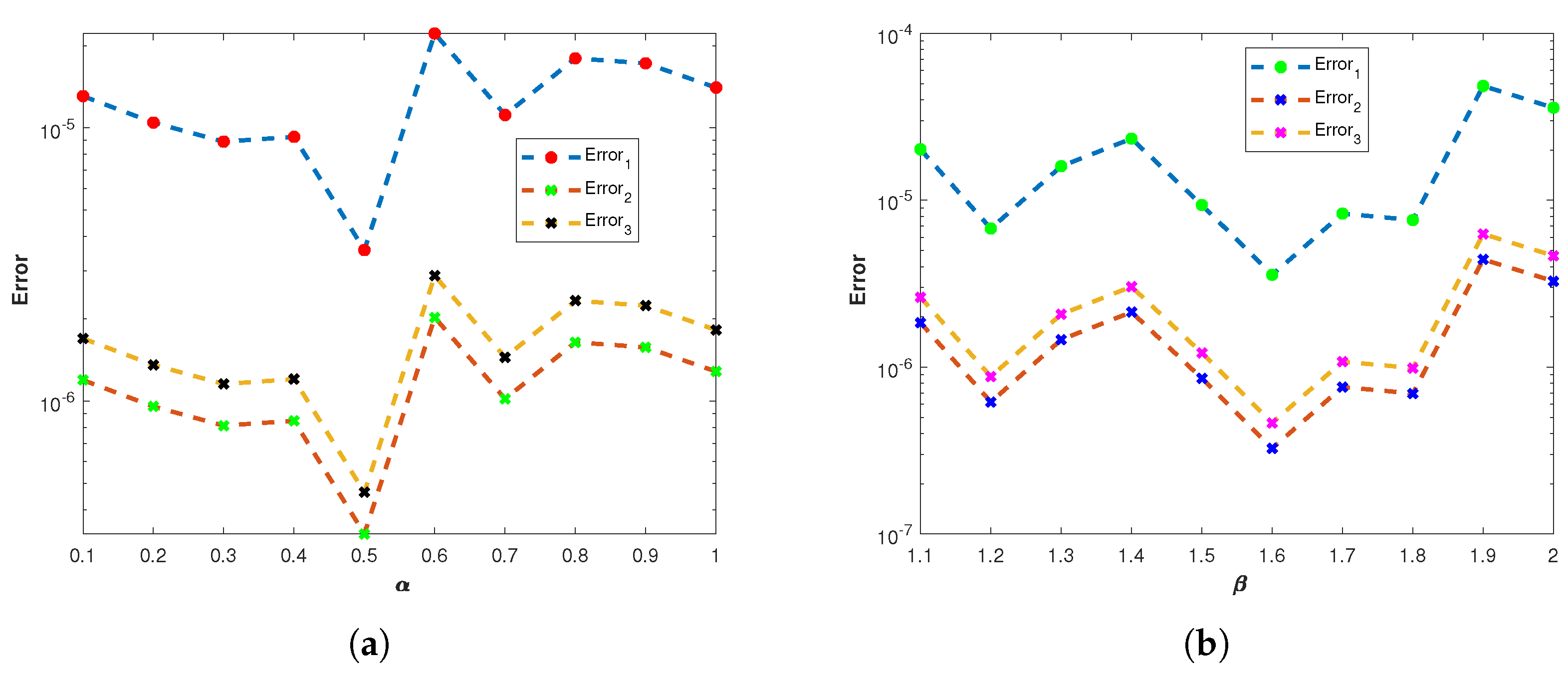
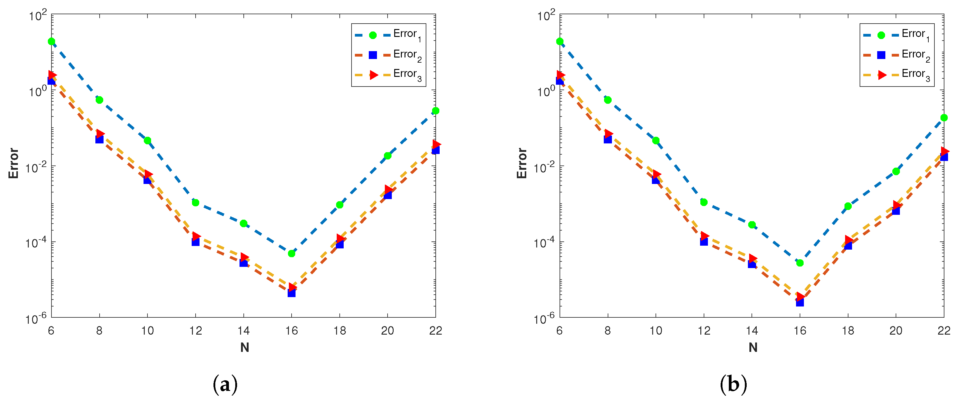
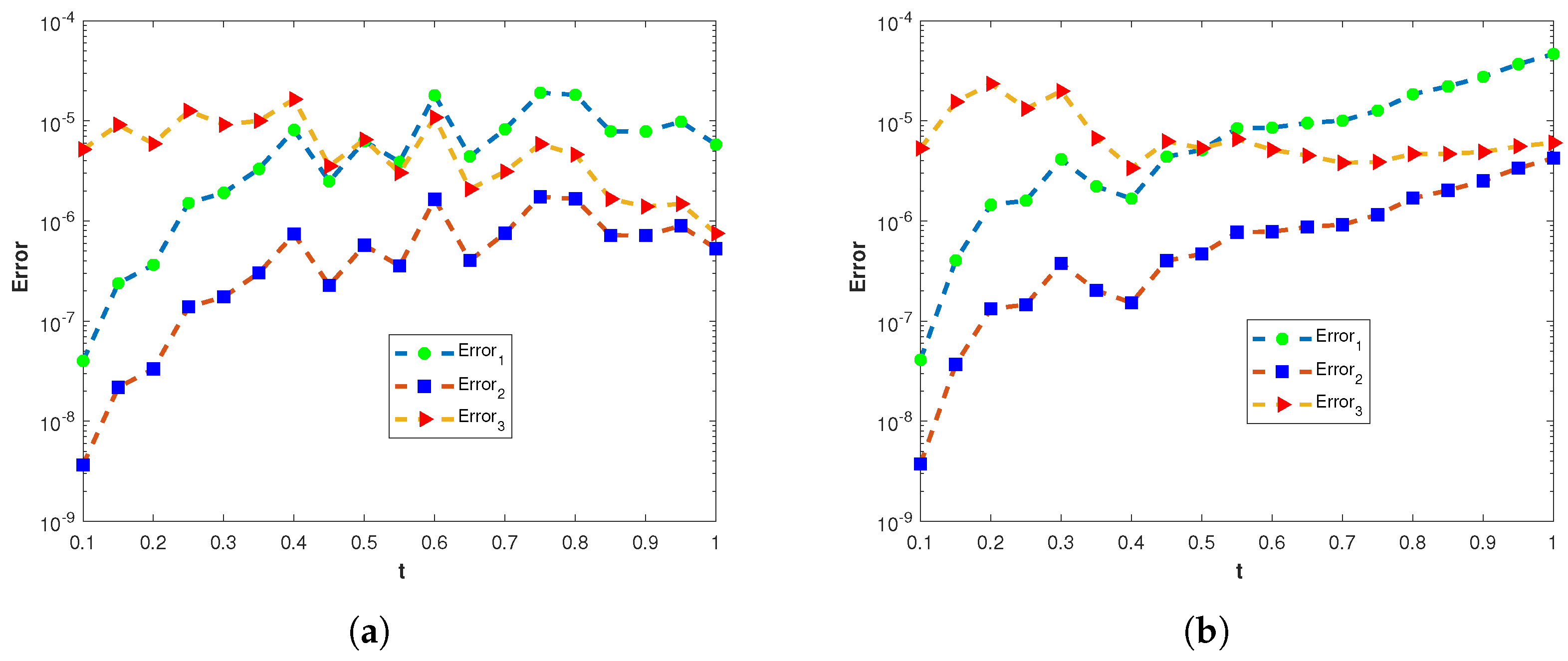
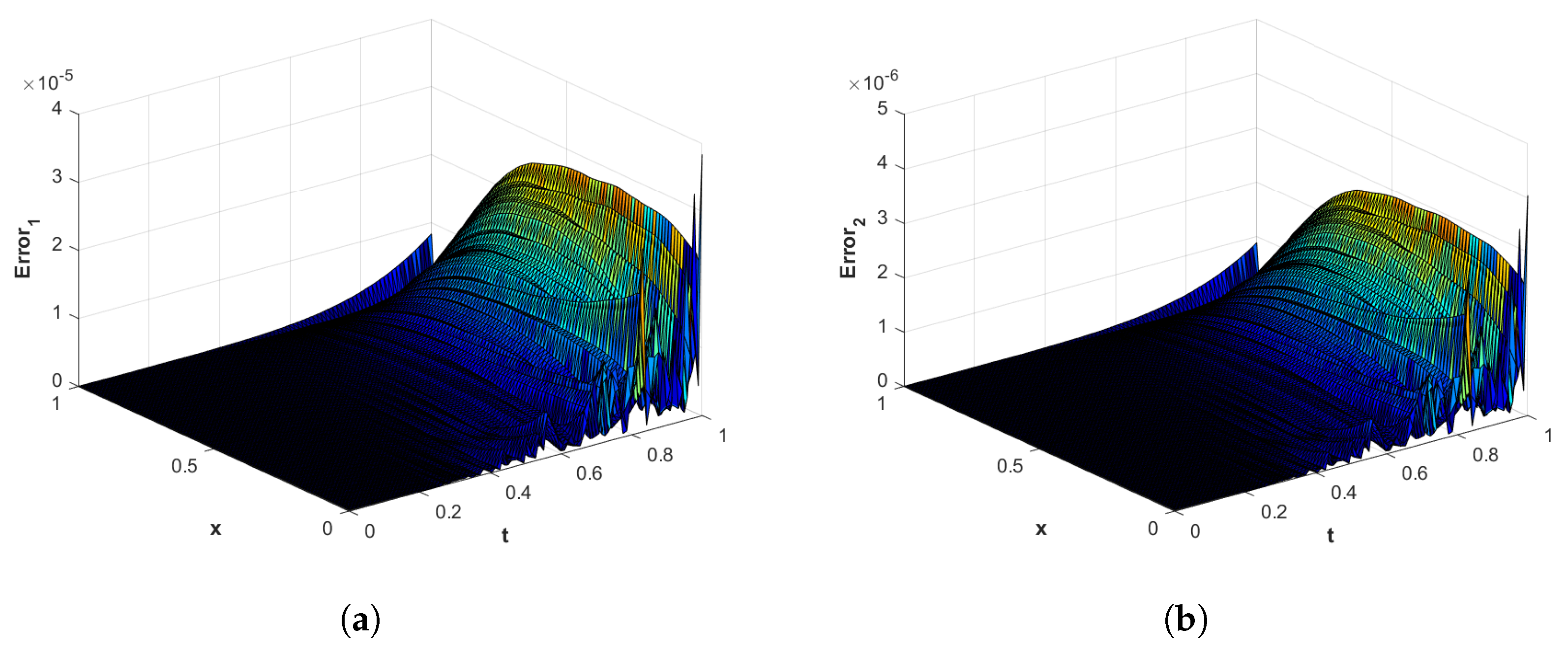
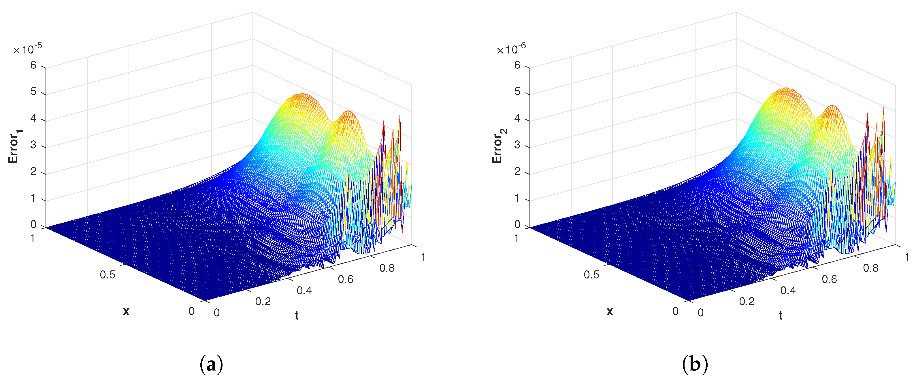
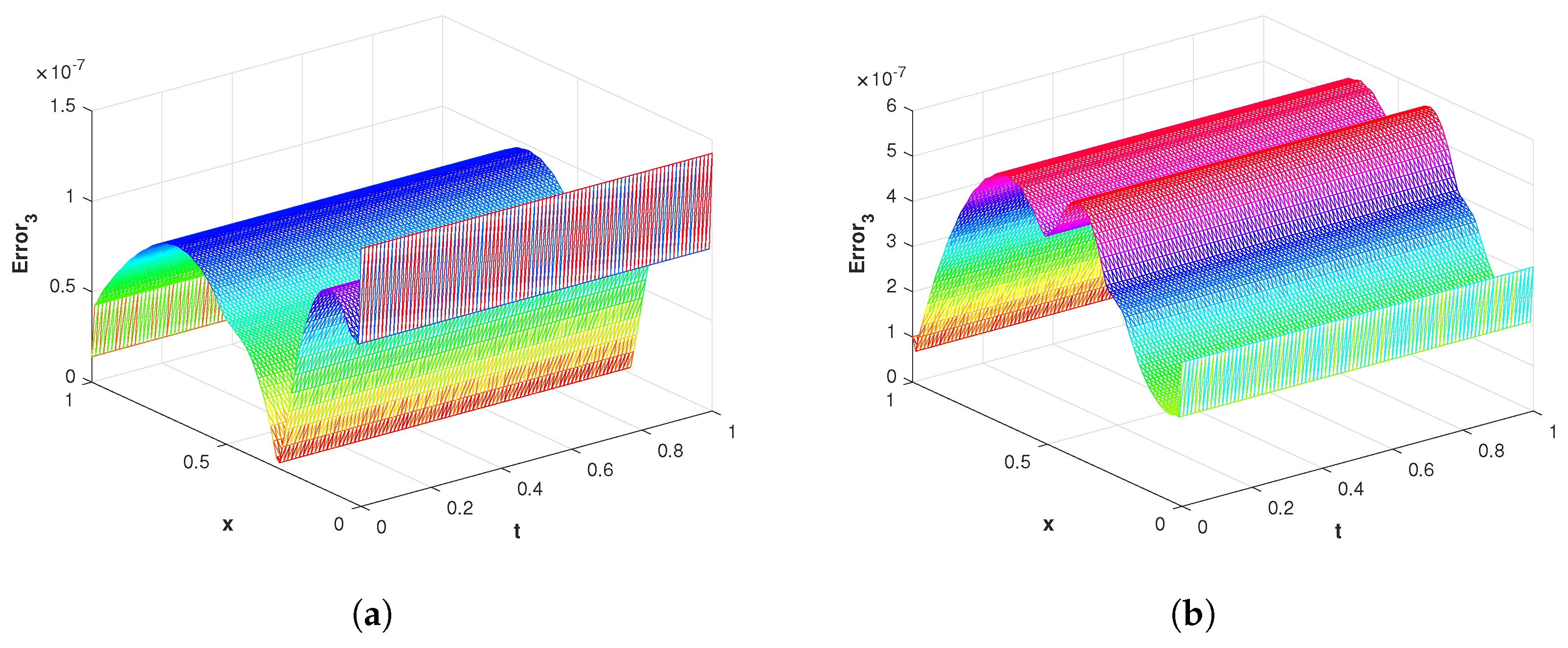
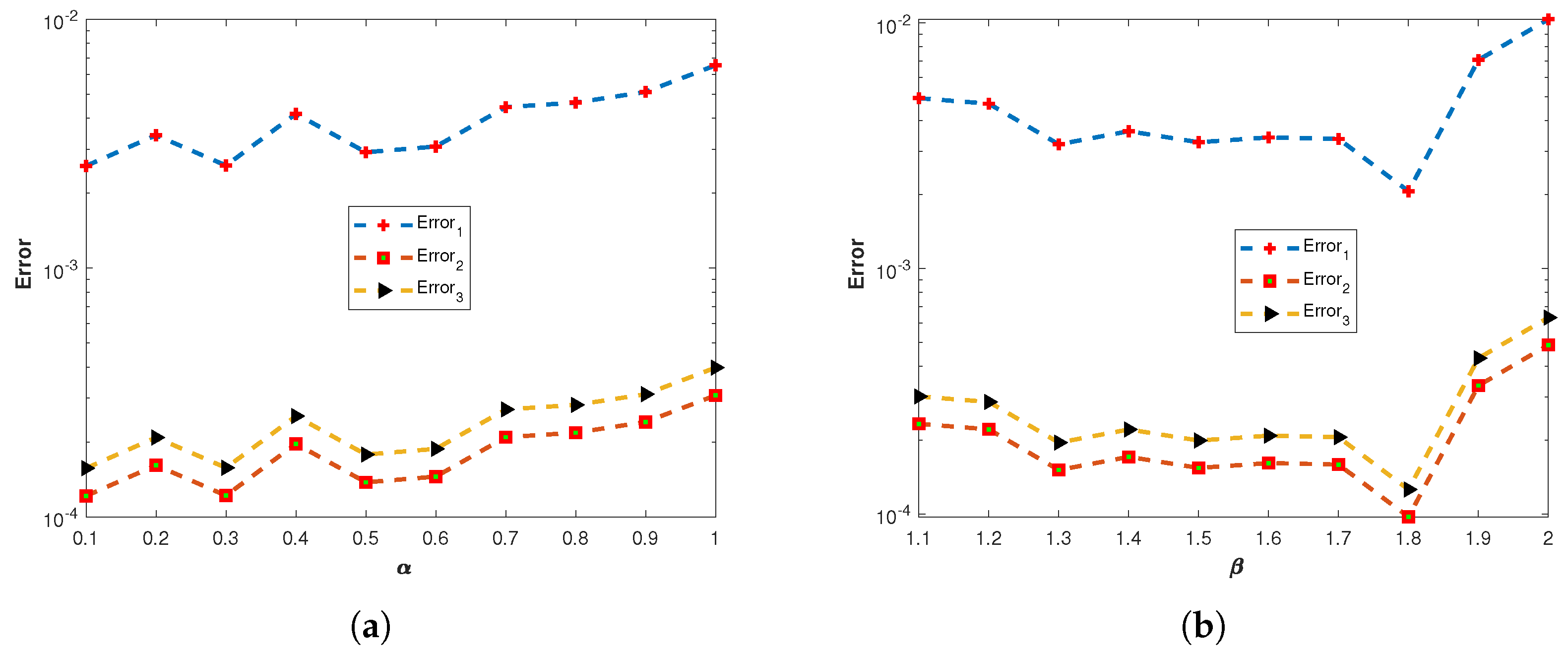
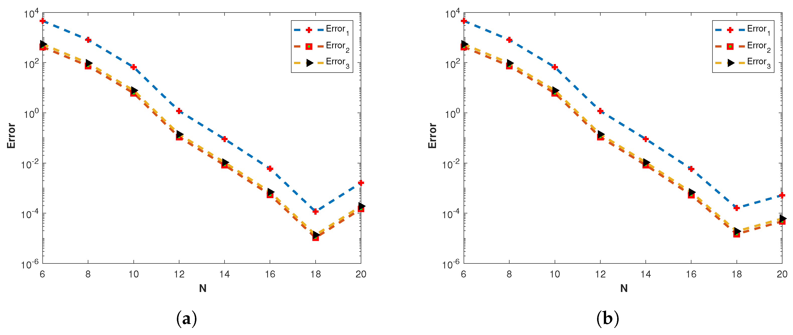
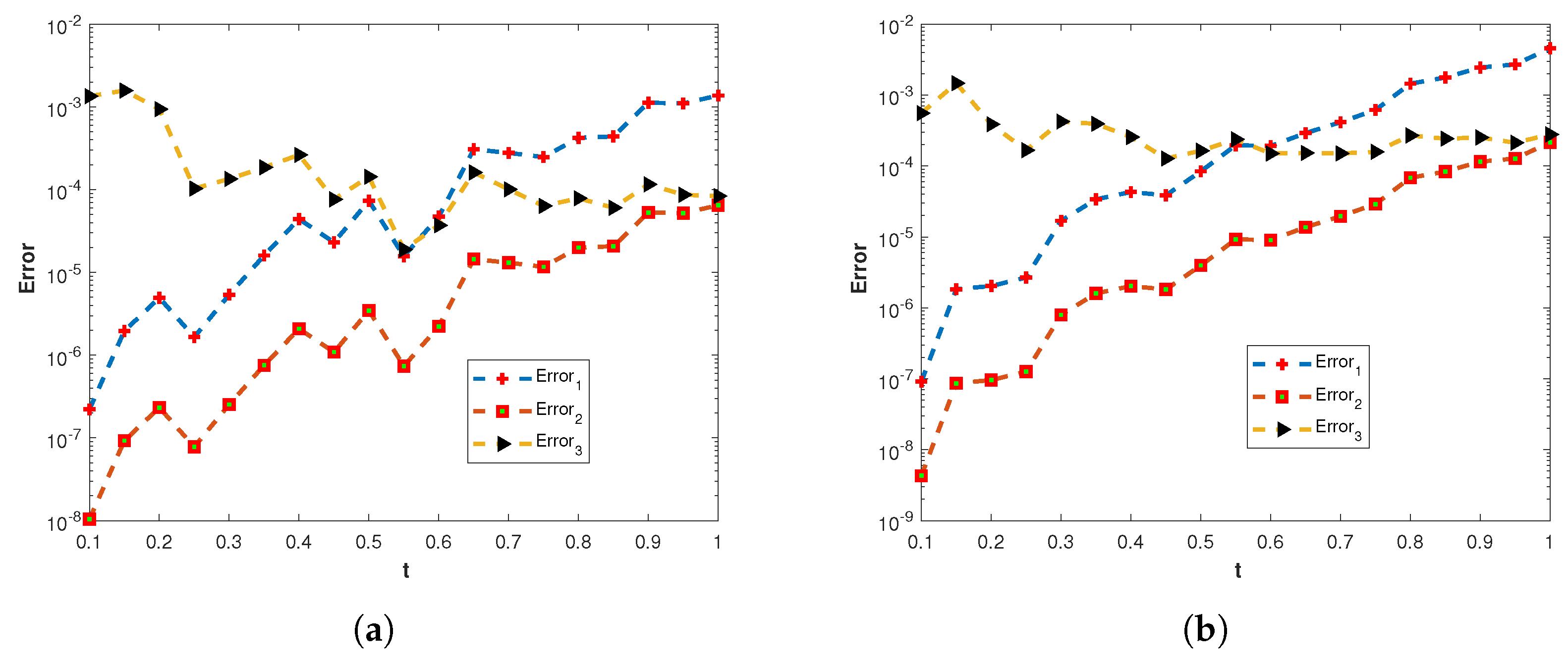
The errors of the proposed method for problem 1 with α = 0.5 , β = 1.1 , and different values of n g , n l , and N using MQ RBF are presented in Table 2, while the errors using GA RBF are presented in Table 3. It is observed that the performance of MQ RBF is better than GA RBF. The results demonstrate that the proposed numerical method is efficient and reliable. Figure 3a,b depict the numerical and analytic solutions of problem 1 with α = 0.5 and β = 1.6 . The surface plots of E r r o r 1 and E r r o r 2 with n g = 70 , n l = 10 , N = 16 , α = 0.5 , and β = 1.9 using MQ RBF are presented in Figure 4a,b; using GA RBF with n g = 70 , n l = 10 , N = 16 , α = 0.5 , and β = 1.7 , they are presented in Figure 5a,b. The surface plots of E r r o r 3 of the proposed method corresponding to problem 1 with n g = 90 , n l = 6 , N = 18 , α = 0.5 , β = 1.9 using MQ RBF and GA RBF are presented in Figure 6a,b. The plots of E r r o r 1 , E r r o r 2 , and E r r o r 3 using MQ RBF for different values of α with β = 1.6 , n g = 120 , n l = 5 , N = 16 are depicted in Figure 7a and for different values of β with α = 0.5 , n g = 120 , n l = 5 , N = 16 are presented in Figure 7b. The plots of E r r o r 1 , E r r o r 2 , and E r r o r 3 for various values of α and β with the same parameters using GA RBF are shown in Figure 8a,b, respectively. The plots of E r r o r 1 , E r r o r 2 , and E r r o r 3 for different values of N with α = 0.5 , β = 1.9 , n g = 120 , n l = 5 using MQ RBF are shown in Figure 9a; using GA RBF, they are presented in Figure 9b. Similarly, the plots of E r r o r 1 , E r r o r 2 , and E r r o r 3 for different values of t with N = 16 , α = 0.7 , β = 1.4 , n g = 120 , n l = 5 using MQ RBF are shown in Figure 10a; using GA RBF, they are shown in Figure 10b. From the data reported in the figures and tables, it is evident that the numerical solution is in good agreement with the analytic solution.
Problem 2.
Consider the following one-dimensional test problem
0 c D t α u ( x , t ) + 0 c D t β u ( x , t ) = Δ u ( x , t ) + f ( x , t ) , 0 x 1 ,
with the exact solution
u ( x , t ) = t ( 3 + α + β ) e x p ( x 2 ) .
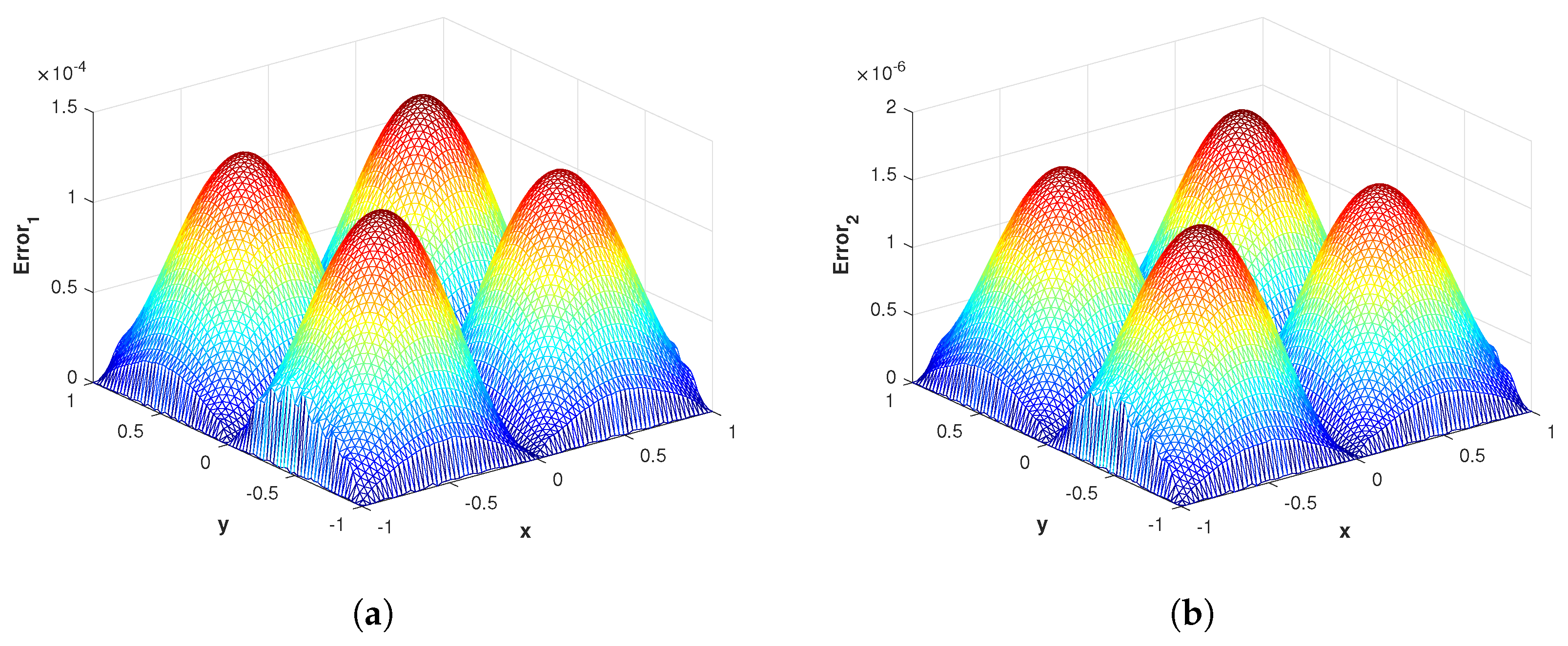
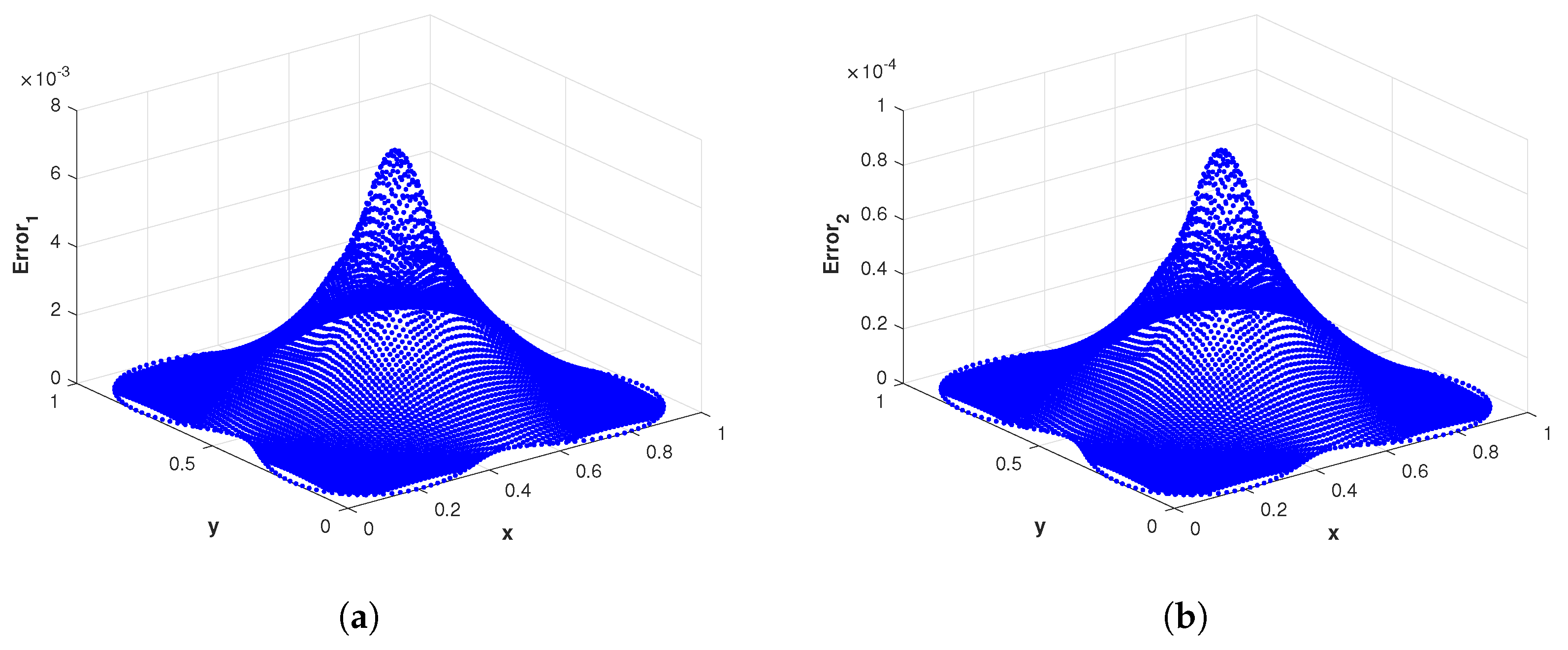
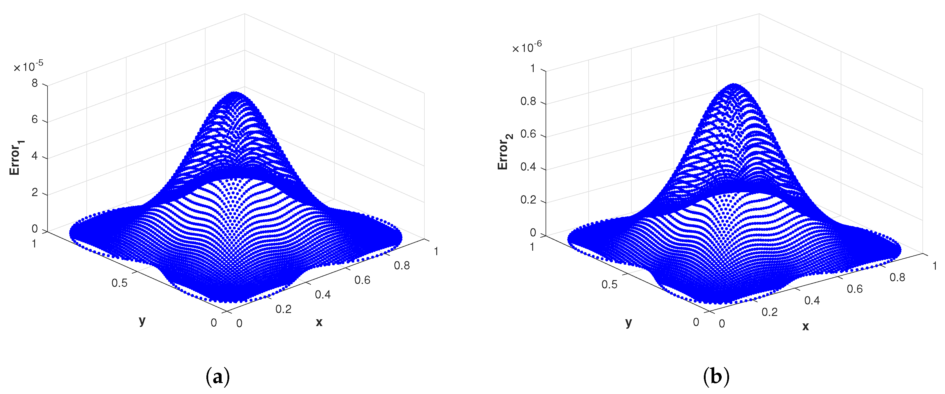
The errors of the proposed method for problem 2 with α = 0.5 , β = 1.5 , and different values of n g , n l , and N using MQ RBF are presented in Table 4; using the GA RBF, they are presented in Table 5. We can see that the method has produced accurate and stable results. The numerical and analytic solutions of problem 2 with α = 0.5 and β = 1.1 are depicted in Figure 11a,b; a nice agreement between the numerical and analytic solutions is observed. The surface plots of E r r o r 1 and E r r o r 2 with n g = 90 , n l = 20 , N = 18 , α = 0.9 and β = 1.3 using MQ RBF are presented in Figure 12a,b. The surface plots of E r r o r 1 and E r r o r 2 with n g = 70 , n l = 10 , N = 16 , α = 0.2 , and β = 1.6 using GA RBF are presented in Figure 13a,b. The surface plot of E r r o r 3 with n g = 90 , n l = 10 , N = 18 , α = 0.2 and β = 1.6 using MQ RBF is presented in Figure 14a and surface plot of E r r o r 3 with n g = 90 , n l = 10 , N = 18 , α = 0.2 and β = 1.6 using GA RBF is presented in Figure 14b. The plots of E r r o r 1 , E r r o r 2 , and E r r o r 3 using MQ RBF for different values of α with β = 1.1 , n g = 120 , n l = 6 , N = 18 are depicted in Figure 15a, and for different values of β with α = 0.9 , n g = 120 , n l = 5 , N = 18 are presented in Figure 15b. The plots of E r r o r 1 , E r r o r 2 , and E r r o r 3 using GA RBF for different values of α with β = 1.6 , n g = 450 , n l = 5 , N = 18 are depicted in Figure 16a, and for different values of β with α = 0.2 , n g = 450 , n l = 5 , N = 18 , are presented in Figure 16b. The plots of E r r o r 1 , E r r o r 2 , and E r r o r 3 using MQ RBF for different values of N with α = 0.9 , β = 1.6 , n g = 450 , n l = 6 are shown in Figure 17a; using GA RBF, they are presented in Figure 17b. The plots of E r r o r 1 , E r r o r 2 , and E r r o r 3 using MQ RBF for different values of t with N = 18 , α = 0.9 , β = 1.1 , n g = 450 , n l = 5 are depicted in Figure 18a; using GA RBF, they are presented in Figure 18b. From the data presented in the tables and figures, it is observed that the proposed method has produced accurate and stable results, and can handle such types of problems efficiently.
Problem 3.
Consider the following two-dimensional test problem
0 c D t α u ( x , y , t ) + 0 c D t β u ( x , y , t ) = Δ u ( x , y , t ) + f ( x , y , t ) , 0 x , y π ,
with analytic solution
u ( x , y , t ) = t 4 sin ( π x ) sin ( π y ) .
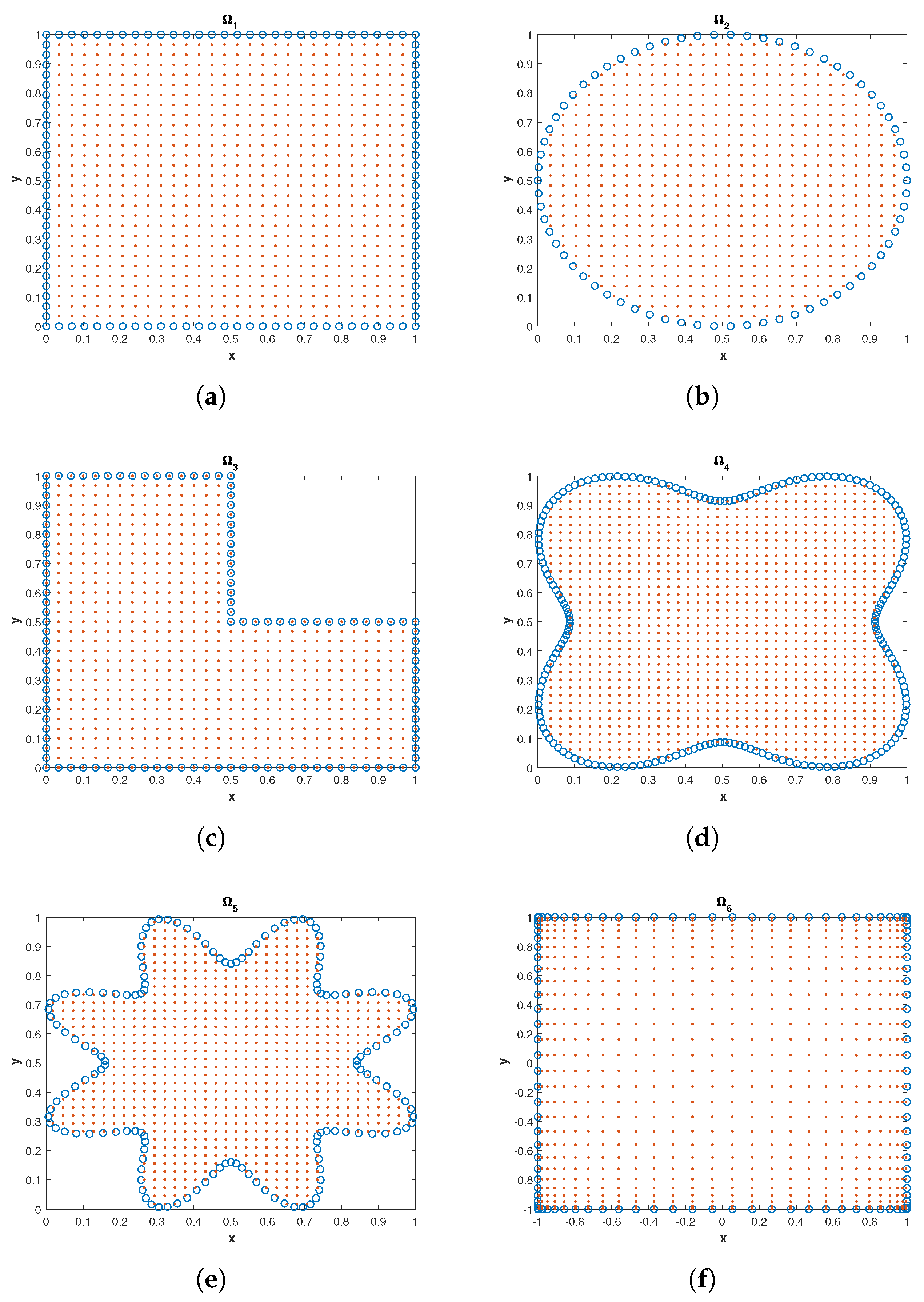
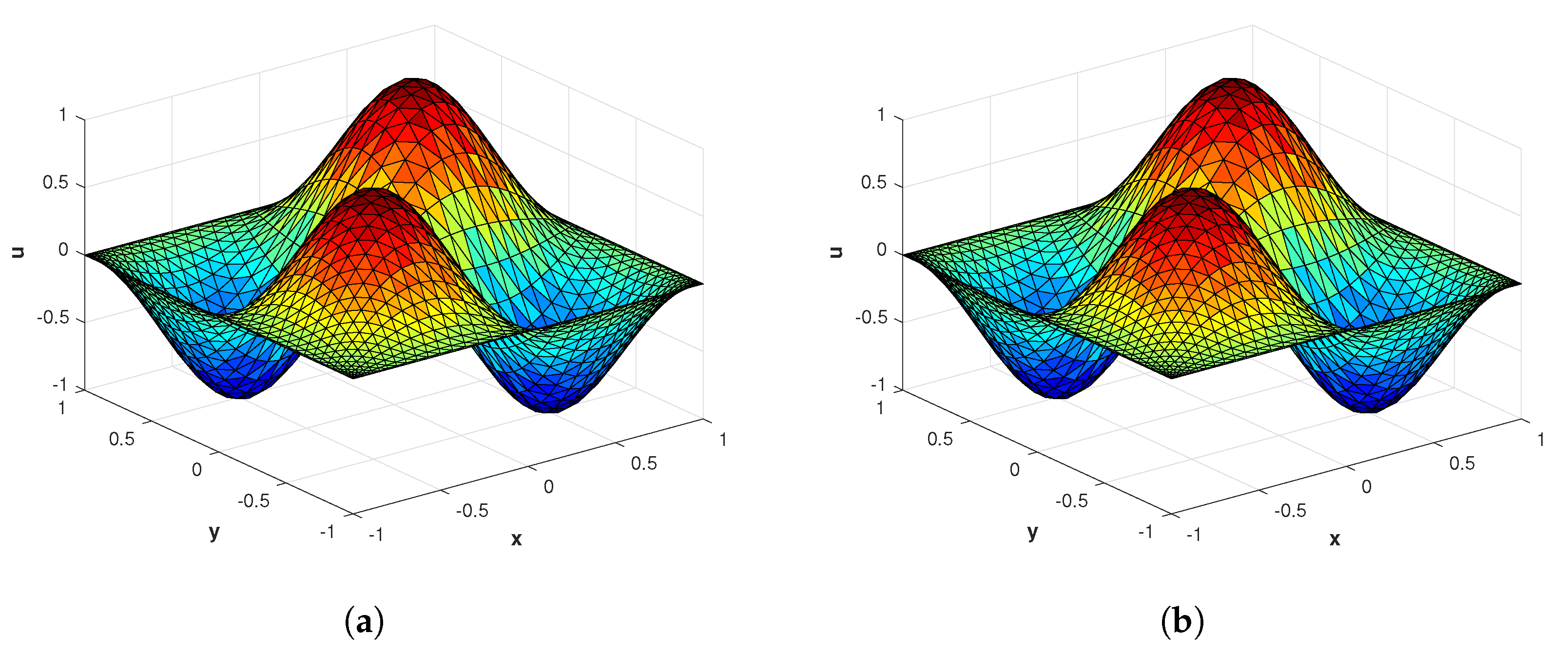
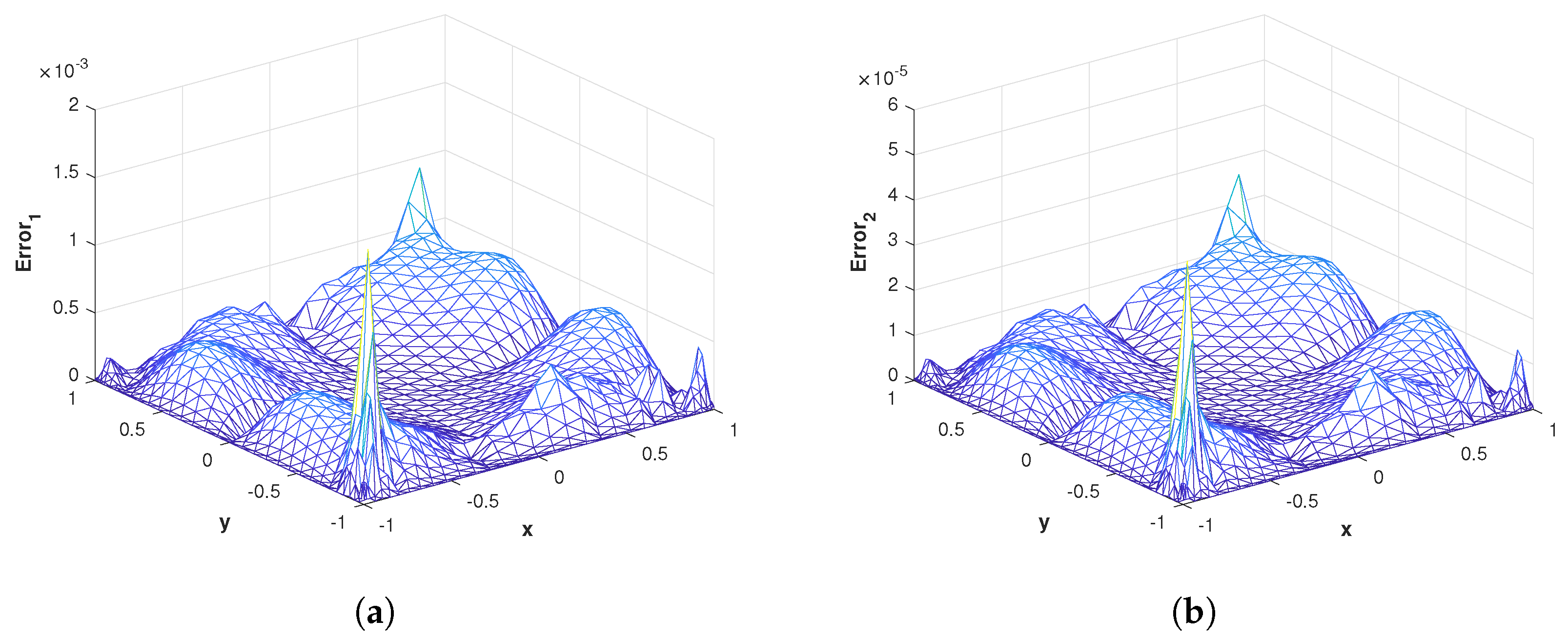
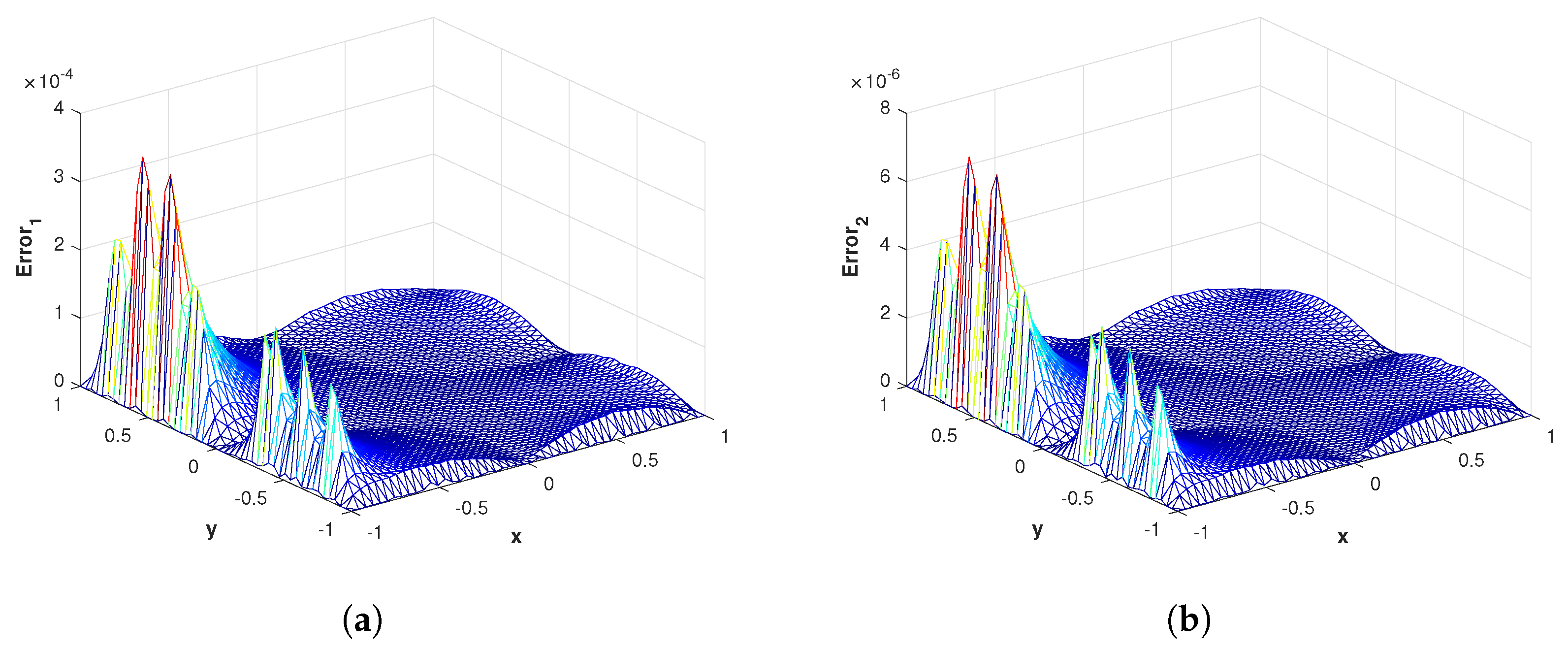
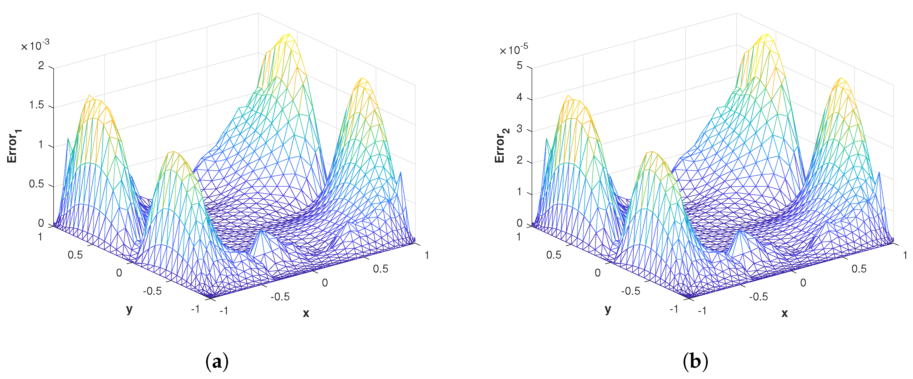
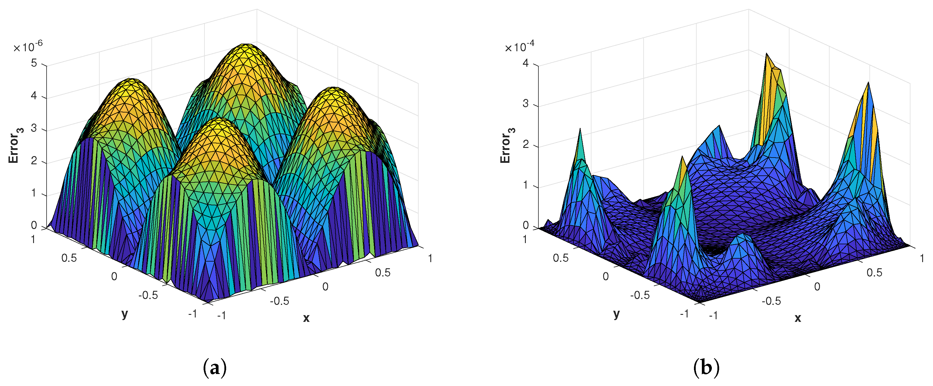
This problem is considered for validating the numerical scheme on domains Ω 1 and Ω 6 as shown in Figure 19a and Figure 19f, respectively. The errors of the proposed method for problem 3 using the MQ RBF on domain Ω 1 are presented in Table 6; using the GA RBF on domain Ω 6 , they are presented in Table 7. It is observed that the method has produced results with acceptable accuracy. The numerical and analytic solutions of problem 3 on domain Ω 1 are depicted in Figure 20a,b, a good agreement between the numerical and analytic solutions is observed. The mesh plots of E r r o r 1 and E r r o r 2 on domain Ω 1 using MQ RBF with n g = 6400 , n l = 35 , N = 18 , α = 0.4 , β = 1.7 are presented in Figure 21a,b. The mesh plots of E r r o r 1 and E r r o r 2 on domain Ω 6 using MQ RBF with n g = 1225 , n l = 35 , N = 18 , α = 0.4 , β = 1.7 are presented in Figure 22a,b. The mesh plots of E r r o r 1 and E r r o r 2 on domain Ω 1 using GA RBF with n g = 2500 , n l = 35 , N = 18 , α = 0.9 , β = 1.1 are presented in Figure 23a,b. The mesh plots of E r r o r 1 and E r r o r 2 on domain Ω 6 using GA RBF with n g = 1600 , n l = 35 , N = 18 , α = 0.5 , β = 1.5 are depicted in Figure 24a,b. The surface plots of E r r o r 3 on domain Ω 1 using MQ RBF with n g = 1600 , n l = 30 , N = 16 , α = 0.5 , β = 1.5 are depicted in Figure 25a and the surface plots of E r r o r 3 on domain Ω 6 using GA RBF with n g = 1600 , n l = 30 , N = 16 , α = 0.5 , β = 1.5 are depicted in Figure 20b. From the obtained results, it is evident that the proposed method can efficiently solve problems with both uniform and non-uniform node distributions.
Problem 4.
Consider the following two-dimensional test problem
0 c D t α u ( x , y , t ) + 0 c D t β u ( x , y , t ) = Δ u ( x , y , t ) + f ( x , y , t ) , 0 x , y 1 ,
with analytic solution
u ( x , y , t ) = ( 1 + t 3 ) ( 1 x 2 y 2 )
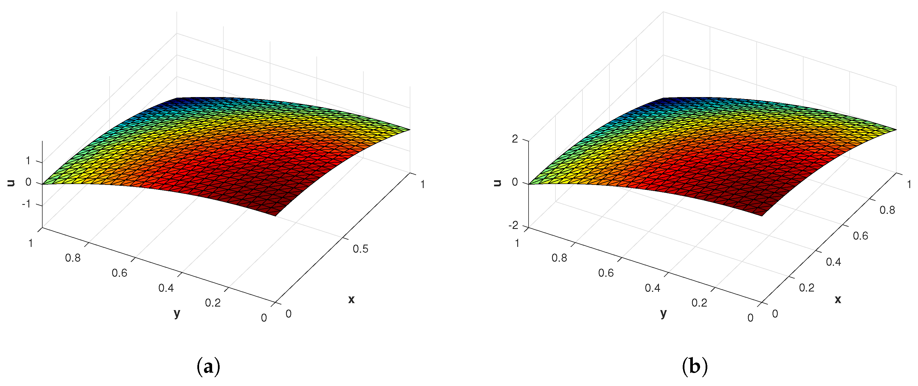
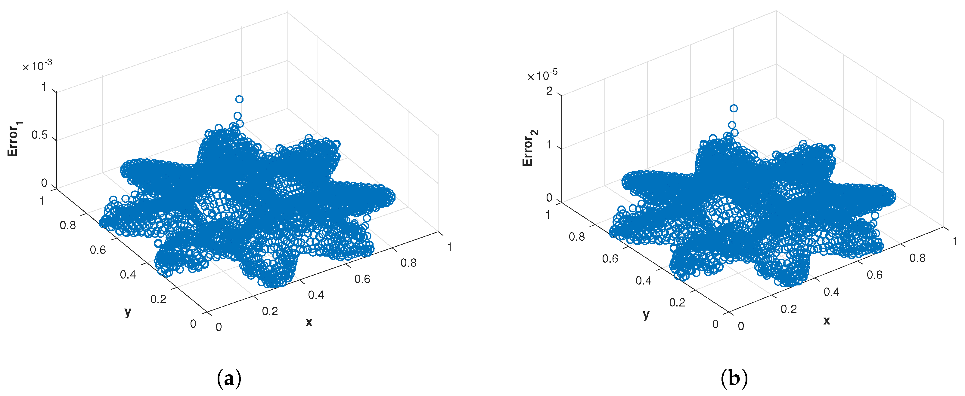
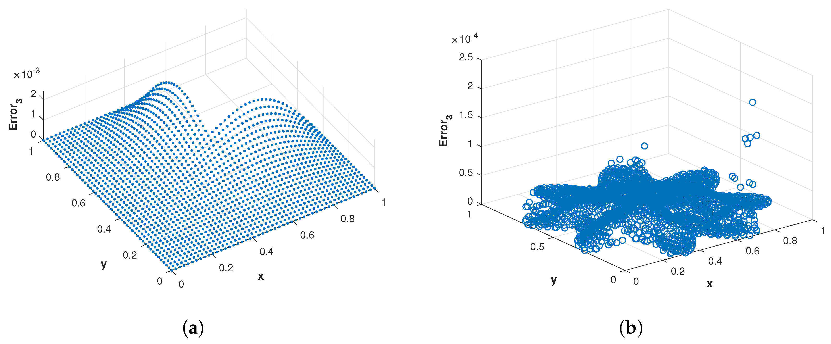
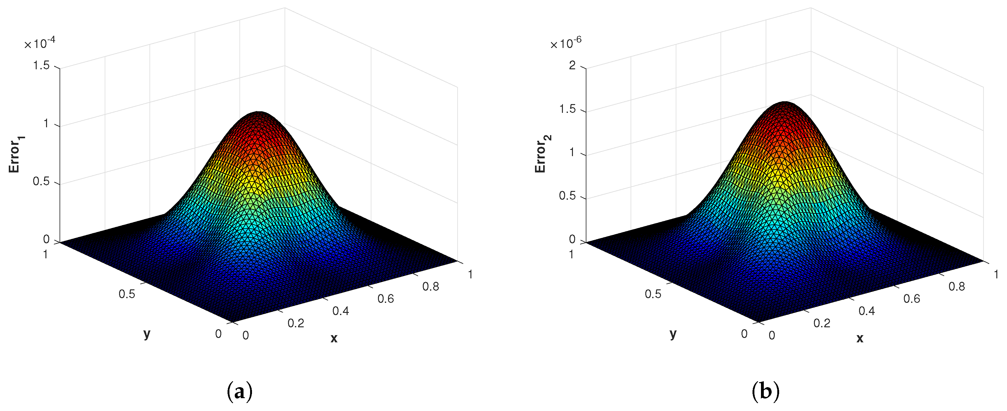
This problem serves to validate the numerical scheme on domains Ω 1 , Ω 3 , and Ω 5 as illustrated in Figure 19a, Figure 19c and Figure 19e, respectively. The errors of the proposed method for problem 4 in domain Ω 1 using MQ RBF are presented in Table 8, while the errors using GA RBF are presented in Table 9. In Table 10 the errors of the proposed method on domain Ω 3 using MQ RBF are presented; in Table 11, the errors on domain Ω 5 using GA RBF are shown. We can see that the proposed method has efficiently solved the considered problem of regular and irregular domains. Figure 26a,b shows the numerical and exact solutions of problem 4 on domain Ω 1 . It is observed that the numerical solution agrees well with the analytic solution. In Figure 27a,b the surface plots of E r r o r 1 and E r r o r 2 using MQ RBF on domain Ω 1 with n g = 4225 , n l = 40 , N = 16 , α = 0.7 , β = 1.9 are depicted. The surface plots of E r r o r 1 and E r r o r 2 using GA RBF on domain Ω 1 with n g = 6400 , n l = 30 , N = 16 , α = 0.2 , β = 1.8 are shown in Figure 28a,b. The scatter plots of E r r o r 1 and E r r o r 2 using MQ RBF on domain Ω 3 with n g = 1281 , n l = 40 , N = 16 , α = 0.7 , β = 1.9 are depicted in Figure 29a,b; using GA RBF, they are presented in Figure 30a,b. The scatter plots of E r r o r 1 and E r r o r 2 using MQ RBF on domain Ω 5 with n g = 3069 , n l = 80 , N = 16 , α = 0.3 , β = 1.6 are shown in Figure 31a,b; using GA RBF with n g = 3069 , n l = 30 , N = 16 , α = 0.3 , β = 1.6 , they are displayed in Figure 32a,b. The scatter plots of E r r o r 3 of the proposed method corresponding to problem 4 using MQ RBF on Ω 3 with n g = 1875 , n l = 30 , N = 18 , α = 0.7 , β = 1.9 are shown in Figure 33a. Similarly, the scatter plots of E r r o r 3 using GA RBF on Ω 5 with n g = 2259 , n l = 30 , N = 18 , α = 0.7 , β = 1.9 are shown in Figure 33b. It can be seen that the performance of the method is excellent for irregular domains as well.
Problem 5.
0 c D t α u ( x , y , t ) + 0 c D t β u ( x , y , t ) = Δ u ( x , y , t ) + f ( x , y , t ) , 0 x , y 1 ,
with analytic solution
u ( x , y , t ) = t 3 ( x 0.5 ) 2 γ + ( y 0.5 ) 2 γ .
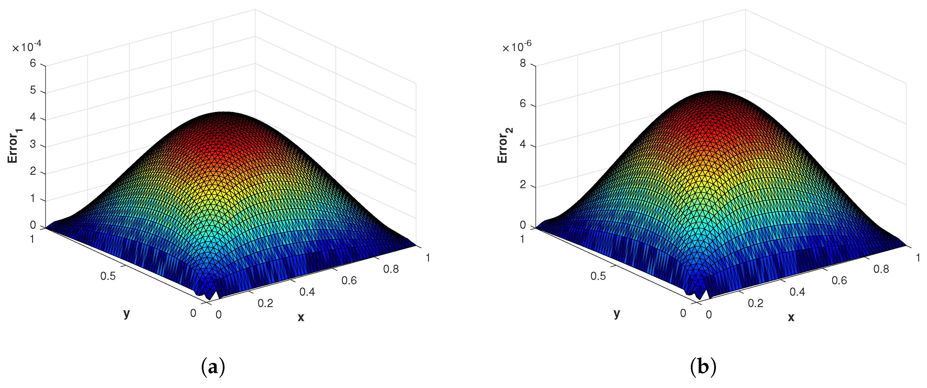
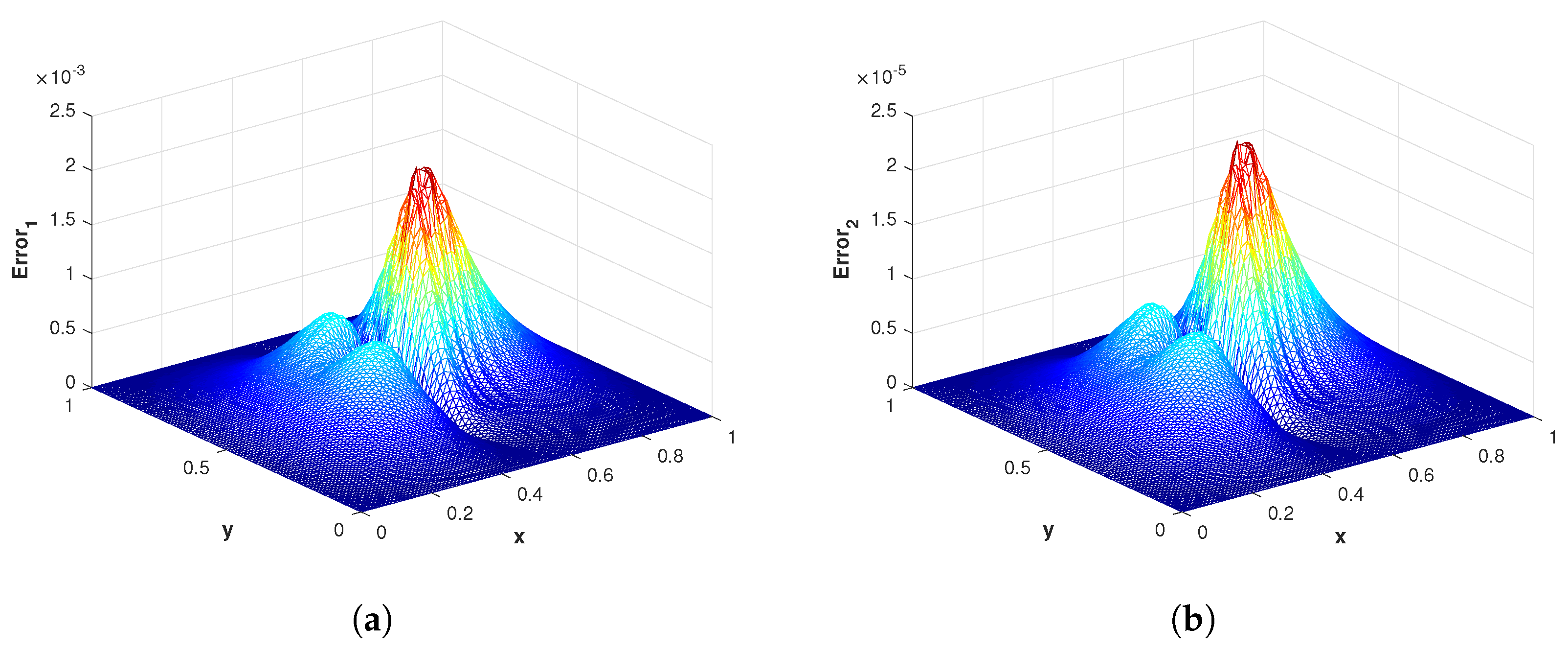
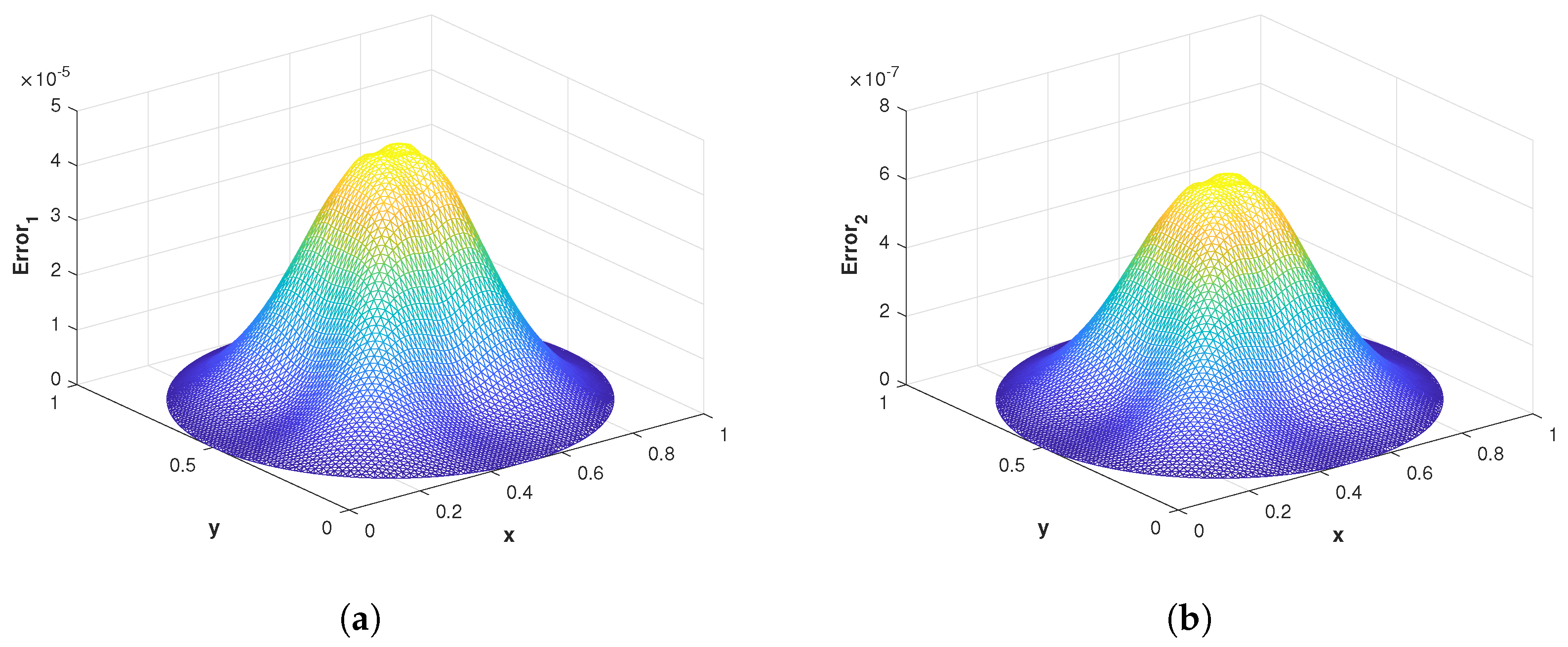
This problem is considered for validating the numerical scheme on domains Ω 1 , Ω 2 and Ω 4 , as shown in Figure 19a, Figure 19b and Figure 19d, respectively. The errors of the proposed method on domain Ω 1 for problem 5 using MQ RBF are presented in Table 12; using GA RBF, they are presented in Table 13. The errors obtained using MQ RBF on domain Ω 2 are presented in Table 14; using GA RBF on domain Ω 4 , they are presented in Table 15. The proposed method produced accurate and stable results on regular as well as irregular domains. The numerical and exact solutions of problem 5 on domain Ω 1 are shown in Figure 34a,b; a nice agreement is observed. The surface plots of E r r o r 1 and E r r o r 2 on domain Ω 1 using MQ RBF with n g = 4900 , n l = 35 , N = 18 , α = 0.7 , β = 1.6 are shown in Figure 35a,b. The surface plots of E r r o r 1 and E r r o r 2 using GA RBF on Ω 1 with n g = 8100 , n l = 35 , N = 18 , α = 0.7 , β = 1.6 are shown in Figure 36a,b. The mesh plots of E r r o r 1 and E r r o r 2 using MQ RBF on domain Ω 2 with n g = 5064 , n l = 30 , N = 18 , α = 0.9 , β = 1.3 are depicted in Figure 37a,b; using GA RBF, they are presented in Figure 38a,b. The scatter plots of E r r o r 1 and E r r o r 2 using MQ RBF on domain Ω 4 with n g = 6393 , n l = 35 , N = 16 , α = 0.7 , β = 1.6 are displayed in Figure 39a,b; using GA RBF, they are presented in Figure 40a,b. The mesh plot of E r r o r 3 using MQ RBF on domain Ω 2 with n g = 5064 , n l = 35 , N = 18 , α = 0.7 , β = 1.6 is presented in Figure 41a; the scatter plot of E r r o r 3 using GA RBF on domain Ω 4 with n g = 6393 , n l = 35 , N = 18 , α = 0.7 , β = 1.6 is presented in Figure 41b. It is observed that the method can solve these types of problems efficiently on regular as well as irregular domains.

5. Conclusions

In this article, an efficient numerical method based on Laplace transform and local radial basis functions for the numerical modeling of fractional mixed diffusion and wave diffusion equations with two Caputo derivatives of order 0 < α < 1 and 1 < β < 2 is proposed. Numerical experiments were conducted in regular and irregular domains with uniform and non-uniform nodes. It is observed that the proposed method effectively solves problems defined on regular and irregular domains with a large number of nodes, requiring less computational time without experiencing any time instability. The results lead to the conclusion that the proposed method is an efficient and reliable technique for the considered problem in all types of domains. However, implementing this computational framework in coupled multi-component systems of partial differential equations remains an open problem. Successful implementation of such a framework could pave the way for further mathematical and biological applications. In future work, we will aim to extend our numerical method to include multiple components of the differential operator of order 2, as introduced in [57]. This will allow us to compare the impact of the errors of the proposed method and the validity of the model with clinical outcomes, thereby facilitating the understanding of complex phenomena.

Author Contributions

Conceptualization, K. and R.K.; methodology, K.; software, R.K. and K.; validation, R.K., K. and S.M.A.; formal analysis, T.A.; investigation, K.; resources, S.M.A.; data curation, S.M.A.; writing—original draft preparation, K.; writing—review and editing, S.M.A. and K.; visualization, R.K.; supervision, K.; project administration, T.A.; funding acquisition, T.A. All authors have read and agreed to the published version of the manuscript.

Funding

This research received no external funding.

Data Availability Statement

All data generated or analyzed during this study are included in this article.

Conflicts of Interest

The authors declare that they have no conflict of interest.

References

  1. Tenreiro Machado, J.A. A probabilistic interpretation of the fractional-order differentiation. Fract. Calc. Appl. Anal. 2003, 6, 73–79. [Google Scholar]
  2. Sun, H.; Chen, W.; Chen, Y. Variable-order fractional differential operators in anomalous diffusion modeling. Phys. Stat. Mech. Its Appl. 2009, 388, 4586–4592. [Google Scholar] [CrossRef]
  3. Torvik, P.J.; Bagley, R.L. On the appearance of the fractional derivative in the behavior of real materials. J. Appl. Mech. 1984, 51, 294–298. [Google Scholar] [CrossRef]
  4. Panda, R.; Dash, M. Fractional generalized splines and signal processing. Signal Process. 2006, 86, 2340–2350. [Google Scholar] [CrossRef]
  5. Benchellal, A.; Poinot, T.; Trigeassou, J.C. Fractional modelling and identification of a thermal process. IFAC Proc. Vol. 2006, 39, 248–253. [Google Scholar] [CrossRef]
  6. Jesus, I.S.; Machado, J.T.; Cunha, J.B. Fractional electrical dynamics in fruits and vegetables. IFAC Proc. Vol. 2006, 39, 308–313. [Google Scholar] [CrossRef]
  7. Lima, M.F.; Tenreiro Machado, J.A.; Crisóstomo, M. Experimental signal analysis of robot impacts in a fractional calculus perspective. J. Adv. Comput. Intell. Intell. Inform. 2007, 11, 1079–1085. [Google Scholar] [CrossRef]
  8. Gorenflo, R.; Luchko, Y.; Mainardi, F. Wright functions as scale-invariant solutions of the diffusion-wave equation. J. Comput. Appl. Math. 2000, 118, 175–191. [Google Scholar] [CrossRef]
  9. Liu, F.; Anh, V.V.; Turner, I.; Zhuang, P. Time fractional advection-dispersion equation. J. Appl. Math. Comput. 2003, 13, 233–245. [Google Scholar] [CrossRef]
  10. Mainardi, F. The fundamental solutions for the fractional diffusion-wave equation. Appl. Math. Lett. 1996, 9, 23–28. [Google Scholar] [CrossRef]
  11. Wyss, W. The fractional diffusion equation. J. Math. Phys. 1986, 27, 2782–2785. [Google Scholar] [CrossRef]
  12. Jiang, H.; Liu, F.; Turner, I.; Burrage, K. Analytical solutions for the multi-term time-fractional diffusion-wave/diffusion equations in a finite domain. Comput. Math. Appl. 2012, 64, 3377–3388. [Google Scholar] [CrossRef]
  13. Momani, S.; Odibat, Z.M. Fractional green function for linear time-fractional inhomogeneous partial differential equations in fluid mechanics. J. Appl. Math. Comput. 2007, 24, 167–178. [Google Scholar] [CrossRef]
  14. Lv, X.; Feng, X. Identifying a Space-Dependent Source Term and the Initial Value in a Time Fractional Diffusion-Wave Equation. Mathematics 2023, 11, 1521. [Google Scholar] [CrossRef]
  15. Diethelm, K.; Ford, J. Numerical solution of the Bagley-Torvik equation. BIT Numer. Math. 2002, 42, 490–507. [Google Scholar] [CrossRef]
  16. Liu, L.; Zhang, S.; Chen, S.; Liu, F.; Feng, L.; Turner, I.; Zhu, J. An Application of the Distributed-Order Time-and Space-Fractional Diffusion-Wave Equation for Studying Anomalous Transport in Comb Structures. Fractal Fract. 2023, 7, 239. [Google Scholar] [CrossRef]
  17. Atta, A.G.; Abd-Elhameed, W.M.; Youssri, Y.H. Shifted fifth-kind Chebyshev polynomials Galerkin-based procedure for treating fractional diffusion-wave equation. Int. J. Mod. Phys. C 2022, 33, 2250102. [Google Scholar] [CrossRef]
  18. Liu, F.; Shen, S.; Anh, V.; Turner, I. Analysis of a discrete non-Markovian random walk approximation for the time fractional diffusion equation. Anziam J. 2004, 46, C488–C504. [Google Scholar] [CrossRef]
  19. Zhao, Y.; Wang, F.; Hu, X.; Shi, Z.; Tang, Y. Anisotropic linear triangle finite element approximation for multi-term time-fractional mixed diffusion and diffusion-wave equations with variable coefficient on 2D bounded domain. Comput. Math. Appl. 2019, 78, 1705–1719. [Google Scholar] [CrossRef]
  20. Liu, Z.; Liu, F.; Zeng, F. An alternating direction implicit spectral method for solving two dimensional multi-term time fractional mixed diffusion and diffusion-wave equations. Appl. Numer. Math. 2019, 136, 139–151. [Google Scholar] [CrossRef]
  21. Agrawal, O.P. Solution for a fractional diffusion-wave equation defined in a bounded domain. Nonlinear Dyn. 2002, 29, 145–155. [Google Scholar] [CrossRef]
  22. Tadjeran, C.; Meerschaert, M.M.; Scheffler, H.P. A second-order accurate numerical approximation for the fractional diffusion equation. J. Comput. Phys. 2006, 213, 205–213. [Google Scholar] [CrossRef]
  23. Li, C.; Chen, A. Numerical methods for fractional partial differential equations. Int. J. Comput. Math. 2018, 95, 1048–1099. [Google Scholar] [CrossRef]
  24. Liu, Y.; Sun, H.; Yin, X.; Feng, L. Fully discrete spectral method for solving a novel multi-term time-fractional mixed diffusion and diffusion-wave equation. Z. Angew. Math. Und Phys. 2020, 71, 1–19. [Google Scholar] [CrossRef]
  25. Dehghan, M.; Manafian, J.; Saadatmandi, A. Solving nonlinear fractional partial differential equations using the homotopy analysis method. Numer. Methods Partial. Differ. Equ. Int. J. 2010, 26, 448–479. [Google Scholar] [CrossRef]
  26. Liu, Q.X.; Gu, Y.; Zhuang, P.; Liu, F.; Nie, Y. An implicit RBF meshless approach for time fractional diffusion equations. Comput. Mech. 2011, 48, 1–12. [Google Scholar] [CrossRef]
  27. Chen, W.; Ye, L.; Sun, H. Fractional diffusion equations by the Kansa method. Comput. Math. Appl. 2010, 59, 1614–1620. [Google Scholar] [CrossRef]
  28. Shivanian, E.; Jafarabadi, A. The spectral meshless radial point interpolation method for solving an inverse source problem of the time-fractional diffusion equation. Appl. Numer. Math. 2018, 129, 1–25. [Google Scholar] [CrossRef]
  29. Shu, C.; Ding, H.; Yeo, K.S. Local radial basis function-based differential quadrature method and its application to solve two-dimensional incompressible Navier-Stokes equations. Comput. Methods Appl. Mech. Eng. 2003, 192, 941–954. [Google Scholar] [CrossRef]
  30. Abbaszadeh, M.; Dehghan, M. Meshless upwind local radial basis function-finite difference technique to simulate the time-fractional distributed-order advection-diffusion equation. Eng. Comput. 2021, 37, 873–889. [Google Scholar] [CrossRef]
  31. Kumar, A.; Bhardwaj, A. A local meshless method for time fractional nonlinear diffusion wave equation. Numer. Algorithms 2020, 85, 1311–1334. [Google Scholar] [CrossRef]
  32. Bhardwaj, A.; Kumar, A. Numerical solution of time fractional tricomi-type equation by an RBF based meshless method. Eng. Anal. Bound. Elem. 2020, 118, 96–107. [Google Scholar] [CrossRef]
  33. Kumar, A.; Bhardwaj, A.; Kumar, B.R. A meshless local collocation method for time fractional diffusion wave equation. Comput. Math. Appl. 2019, 78, 1851–1861. [Google Scholar] [CrossRef]
  34. Kumar, A.; Bhardwaj, A.; Dubey, S. A local meshless method to approximate the time-fractional telegraph equation. Eng. Comput. 2021, 37, 3473–3488. [Google Scholar] [CrossRef]
  35. Hosseini, V.R.; Shivanian, E.; Chen, W. Local radial point interpolation (MLRPI) method for solving time fractional diffusion-wave equation with damping. J. Comput. Phys. 2016, 312, 307–332. [Google Scholar] [CrossRef]
  36. Salehi, R. A meshless point collocation method for 2-D multi-term time fractional diffusion-wave equation. Numer. Algorithms 2017, 74, 1145–1168. [Google Scholar] [CrossRef]
  37. Aslefallah, M.; Shivanian, E. An efficient meshless method based on RBFs for the time fractional diffusion-wave equation. Afr. Mat. 2018, 29, 1203–1214. [Google Scholar] [CrossRef]
  38. Yang, J.Y.; Zhao, Y.M.; Liu, N.; Bu, W.P.; Xu, T.L.; Tang, Y.F. An implicit MLS meshless method for 2-D time dependent fractional diffusion-wave equation. Appl. Math. Model. 2015, 39, 1229–1240. [Google Scholar] [CrossRef]
  39. Wei, S.; Chen, W.; Zhang, Y.; Wei, H.; Garrard, R.M. A local radial basis function collocation method to solve the variable-order time fractional diffusion equation in a two-dimensional irregular domain. Numer. Methods Partial. Differ. Equ. 2018, 34, 1209–1223. [Google Scholar] [CrossRef]
  40. Kamran, K.; Shah, Z.; Kumam, P.; Alreshidi, N.A. A meshless method based on the laplace transform for the 2D multi-term time fractional partial integro-differential equation. Mathematics 2020, 8, 1972. [Google Scholar]
  41. Kamran; Ali, A.; Gómez-Aguilar, J.F. A transform based local RBF method for 2D linear PDE with Caputo-Fabrizio derivative. Comptes Rendus. Mathématique 2020, 358, 831–842. [Google Scholar]
  42. Sarra, S.A. A local radial basis function method for advection-diffusion-reaction equations on complexly shaped domains. Appl. Math. Comput. 2012, 218, 9853–9865. [Google Scholar] [CrossRef]
  43. Sun, Z.Z.; Ji, C.C.; Du, R. A new analytical technique of the L-type difference schemes for time fractional mixed sub-diffusion and diffusion-wave equations. Appl. Math. Lett. 2020, 102, 106115. [Google Scholar] [CrossRef]
  44. Feng, L.; Liu, F.; Turner, I. Finite difference/finite element method for a novel 2D multi-term time-fractional mixed sub-diffusion and diffusion-wave equation on convex domains. Commun. Nonlinear Sci. Numer. Simul. 2019, 70, 354–371. [Google Scholar] [CrossRef]
  45. Bhardwaj, A.; Kumar, A. A numerical solution of time-fractional mixed diffusion and diffusion-wave equation by an RBF-based meshless method. Eng. Comput. 2020, 38, 1883–1903. [Google Scholar] [CrossRef]
  46. Gu, X.M.; Wu, S.L. A parallel-in-time iterative algorithm for Volterra partial integro-differential problems with weakly singular kernel. J. Comput. Phys. 2020, 417, 109576. [Google Scholar] [CrossRef]
  47. Sarra, S.A.; Kansa, E.J. Multiquadric radial basis function approximation methods for the numerical solution of partial differential equations. Adv. Comput. Mech. 2009, 2, 220. [Google Scholar]
  48. Schaback, R. Error estimates and condition numbers for radial basis function interpolation. Adv. Comput. Math. 1995, 3, 251–264. [Google Scholar] [CrossRef]
  49. Trefethen, L.N.; Bau, D., III. Numerical Linear Algebra; Siam: Philadelphia, PA, USA, 1997; Volume 50. [Google Scholar]
  50. Stehfest, H. Algorithm 368: Numerical inversion of Laplace transforms [D5]. Commun. ACM 1970, 13, 47–49. [Google Scholar] [CrossRef]
  51. Stehfest, H. Remark on algorithm 368: Numerical inversion of Laplace transforms. Commun. ACM 1970, 13, 624. [Google Scholar] [CrossRef]
  52. Davies, B.; Martin, B. Numerical inversion of the Laplace transform: A survey and comparison of methods. J. Comput. Phys. 1979, 33, 1–32. [Google Scholar] [CrossRef]
  53. Kuznetsov, A. On the Convergence of the Gaver–Stehfest Algorithm. SIAM J. Numer. Anal. 2013, 51, 2984–2998. [Google Scholar] [CrossRef]
  54. Abate, J.; Valkó, P.P. Multi-precision Laplace transform inversion. Int. J. Numer. Methods Eng. 2004, 60, 979–993. [Google Scholar] [CrossRef]
  55. Abate, J.; Whitt, W. A unified framework for numerically inverting Laplace transforms. INFORMS J. Comput. 2006, 18, 408–421. [Google Scholar] [CrossRef]
  56. Fu, Z.J.; Chen, W.; Yang, H.T. Boundary particle method for Laplace transformed time fractional diffusion equations. J. Comput. Phys. 2013, 235, 52–66. [Google Scholar] [CrossRef]
  57. Alzahrani, T. Spatio-temporal modeling of immune response to SARS-CoV-2 infection. Mathematics 2021, 9, 3274. [Google Scholar] [CrossRef]
Figure 1. (a) The MQ RBF plot in the domain [ 5 , 5 ] with ε = 0.5 ; (b) the GA RBF plot in the domain [ 5 , 5 ] with ε = 0.5 ; (c) the IMQ RBF plot in the domain [ 5 , 5 ] with ε = 0.5 ; (d) the TPS RBF plot in the domain [ 5 , 5 ] with ε = 0.5 .
Fractalfract 07 00381 g001
Figure 2. A stencil for n l = 10 , red corresponds to the boundary node and brown to the interior node.
Fractalfract 07 00381 g002
Figure 3. (a) The numerical solution of problem 1 with α = 0.5 , β = 1.6 . (b) The exact solution of problem 1 with α = 0.5 , β = 1.6 .
Fractalfract 07 00381 g003
Figure 4. (a) The surface plot of E r r o r 1 of the proposed method corresponding to problem 1 with n g = 70 , n l = 10 , N = 16 , α = 0.5 , β = 1.9 using MQ RBF. (b) The surface plot of E r r o r 2 of the proposed method corresponding to problem 1 with n g = 70 , n l = 10 , N = 16 , α = 0.5 , β = 1.9 using MQ RBF.
Fractalfract 07 00381 g004
Figure 5. (a) The mesh plot of E r r o r 1 of the proposed method corresponding to problem 1 with n g = 70 , n l = 10 , N = 16 , α = 0.5 , β = 1.7 using GA RBF. (b) The mesh plot of E r r o r 2 of the proposed method corresponding to problem 1 with n g = 70 , n l = 10 , N = 16 , α = 0.5 , β = 1.7 using GA RBF.
Fractalfract 07 00381 g005
Figure 6. (a) The surface plot of E r r o r 3 of the proposed method corresponding to problem 1 with n g = 90 , n l = 6 , N = 18 , α = 0.5 , β = 1.9 using MQ RBF. (b) The surface plot of E r r o r 3 of the proposed method corresponding to problem 1 with n g = 90 , n l = 6 , N = 18 , α = 0.5 , β = 1.9 using GA RBF.
Fractalfract 07 00381 g006
Figure 7. (a) The plots of E r r o r 1 , E r r o r 2 , and E r r o r 3 of the proposed method corresponding to problem 1 with various values of α and β = 1.6 , n g = 120 , n l = 5 , N = 16 using the MQ RBF. (b) The plots E r r o r 1 , E r r o r 2 , and E r r o r 3 of the proposed method corresponding to problem 1 with various values of β and α = 0.5 , n g = 120 , n l = 5 , N = 16 using the MQ RBF.
Fractalfract 07 00381 g007
Figure 8. (a) The plots of E r r o r 1 , E r r o r 2 , and E r r o r 3 of the proposed method corresponding to problem 1 with various values of α and β = 1.6 , n g = 120 , n l = 5 , N = 16 using the GA RBF. (b) The plots E r r o r 1 , E r r o r 2 , and E r r o r 3 of the proposed method corresponding to problem 1 with various values of β and α = 0.5 , n g = 120 , n l = 5 , N = 16 using the GA RBF.
Fractalfract 07 00381 g008
Figure 9. (a) The plots of E r r o r 1 , E r r o r 2 , and E r r o r 3 of the proposed method corresponding to problem 1 with various values of N and α = 0.5 , β = 1.9 , n g = 120 , n l = 5 using the MQ RBF. (b) The plots E r r o r 1 , E r r o r 2 , and E r r o r 3 of the proposed method corresponding to problem 1 with various values of N and α = 0.5 , β = 1.9 , n g = 120 , n l = 5 using the GA RBF.
Fractalfract 07 00381 g009
Figure 10. (a) The plots of E r r o r 1 , E r r o r 2 , and E r r o r 3 of the proposed method corresponding to problem 1 with various values of t and N = 16 , α = 0.7 , β = 1.4 , n g = 120 , n l = 5 using the MQ RBF. (b) The plots E r r o r 1 , E r r o r 2 , and E r r o r 3 of the proposed method corresponding to problem 1 with various values of t and N = 16 , α = 0.7 , β = 1.4 , n g = 120 , n l = 5 using the GA RBF.
Fractalfract 07 00381 g010
Figure 11. (a) The numerical solution of problem 2 with α = 0.5 , β = 1.1 . (b) The exact solution of problem 2 with α = 0.5 , β = 1.1 .
Fractalfract 07 00381 g011
Figure 12. (a) The surface plot of E r r o r 1 of the proposed method corresponding to problem 2 with n g = 90 , n l = 20 , N = 18 , α = 0.9 , β = 1.3 using MQ RBF. (b) The surface plot of E r r o r 2 of the proposed method corresponding to problem 2 with n g = 90 , n l = 20 , N = 18 , α = 0.9 , β = 1.3 using MQ RBF.
Fractalfract 07 00381 g012
Figure 13. (a) The mesh plot of E r r o r 1 of the proposed method corresponding to problem 2 with n g = 90 , n l = 10 , N = 18 , α = 0.2 , β = 1.6 using GA RBF. (b) The mesh plot of E r r o r 2 of the proposed method corresponding to problem 2 with n g = 90 , n l = 10 , N = 18 , α = 0.2 , β = 1.6 using GA RBF.
Fractalfract 07 00381 g013
Figure 14. (a) The surface plot of E r r o r 3 of the proposed method corresponding to problem 2 with N = 18 , α = 0.2 , β = 1.6 , n g = 90 , n l = 10 using MQ RBF. (b) The surface plot of E r r o r 3 of the proposed method corresponding to problem 2 with N = 18 α = 0.2 , β = 1.6 , n g = 90 , n l = 10 using GA RBF.
Fractalfract 07 00381 g014
Figure 15. (a) The plots of E r r o r 1 , E r r o r 2 , and E r r o r 3 of the proposed method corresponding to problem 2 with various values of α and β = 1.1 , n g = 120 , n l = 6 , N = 18 using MQ RBF. (b) The plots E r r o r 1 , E r r o r 2 , and E r r o r 3 of the proposed method corresponding to problem 2 with various values of β and α = 0.9 , n g = 120 , n l = 6 , N = 18 using MQ RBF.
Fractalfract 07 00381 g015
Figure 16. (a) The plots of E r r o r 1 , E r r o r 2 , and E r r o r 3 of the proposed method corresponding to problem 2 with various values of α and β = 1.6 , n g = 450 , n l = 5 , N = 18 using GA RBF. (b) The plots E r r o r 1 , E r r o r 2 , and E r r o r 3 of the proposed method corresponding to problem 2 with various values of β and α = 0.2 , n g = 450 , n l = 5 , N = 18 using GA RBF.
Fractalfract 07 00381 g016
Figure 17. (a) The plots of E r r o r 1 , E r r o r 2 , and E r r o r 3 of the proposed method corresponding to problem 2 with various values of N and α = 0.5 , β = 1.6 , n g = 120 , n l = 5 using MQ RBF. (b) The plots E r r o r 1 , E r r o r 2 , and E r r o r 3 of the proposed method corresponding to problem 2 with various values of N and α = 0.5 , β = 1.6 , n g = 120 , n l = 5 using GA RBF.
Fractalfract 07 00381 g017
Figure 18. (a) The plots of E r r o r 1 , E r r o r 2 , and E r r o r 3 of the proposed method corresponding to problem 2 with various values of t and N = 18 , α = 0.9 , β = 1.1 , n g = 450 , n l = 5 using MQ RBF. (b) The plots E r r o r 1 , E r r o r 2 , and E r r o r 3 of the proposed method corresponding to problem 2 with various values of t and N = 18 α = 0.9 , β = 1.1 , n g = 450 , n l = 5 using GA RBF.
Fractalfract 07 00381 g018
Figure 19. (a) Uniform nodes distribution in the square domain; (b) Uniform nodes distribution in the circular domain; (c) Uniform nodes distribution in the L shaped domain; (d) Uniform nodes distribution in the nut shaped domain; (e) Uniform nodes distribution in the star shaped domain; (f) Chebyshev nodes distribution in the square domain.
Fractalfract 07 00381 g019
Figure 20. (a) The numerical solution of problem 3 on Ω 1 . (b) The exact solution of problem 3 on Ω 1 .
Fractalfract 07 00381 g020
Figure 21. (a) The mesh plot of E r r o r 1 of the proposed method corresponding to problem 3 using MQ RBF on Ω 1 with n g = 6400 , n l = 35 , N = 18 , α = 0.4 , β = 1.7 . (b) The mesh plot of E r r o r 2 of the proposed method corresponding to problem 3 using MQ RBF on Ω 1 with n g = 6400 , n l = 35 , N = 18 , α = 0.4 , β = 1.7 .
Fractalfract 07 00381 g021
Figure 22. (a) The mesh plot of E r r o r 1 of the proposed method corresponding to problem 3 using MQ RBF on Ω 6 with n g = 1225 , n l = 35 , N = 18 , α = 0.4 , β = 1.7 . (b) The mesh plot of E r r o r 2 of the proposed method corresponding to problem 3 using MQ RBF on Ω 6 with n g = 1225 , n l = 35 , N = 18 , α = 0.4 , β = 1.7 .
Fractalfract 07 00381 g022
Figure 23. (a) The mesh plot of E r r o r 1 of the proposed method corresponding to problem 3 using GA RBF on Ω 1 with n g = 2500 , n l = 35 , N = 18 , α = 0.9 , β = 1.1 . (b) The mesh plot of E r r o r 2 of the proposed method corresponding to problem 3 using GA RBF on Ω 1 with n g = 2500 , n l = 35 , N = 18 , α = 0.9 , β = 1.1 .
Fractalfract 07 00381 g023
Figure 24. (a) The mesh plot of E r r o r 1 of the proposed method corresponding to problem 3 using GA RBF on Ω 6 with n g = 1600 , n l = 35 , N = 18 , α = 0.5 , β = 1.5 . (b) The mesh plot of E r r o r 2 of the proposed method corresponding to problem 3 using GA RBF on Ω 6 with n g = 1600 , n l = 35 , N = 18 , α = 0.5 , β = 1.5 .
Fractalfract 07 00381 g024
Figure 25. (a) The surface plot of E r r o r 3 of the proposed method corresponding to problem 3 using MQ RBF on Ω 1 with n g = 1600 , n l = 30 , N = 16 , α = 0.5 , β = 1.5 . (b) The surface plot of E r r o r 3 of the proposed method corresponding to problem 3 using GA RBF on Ω 6 with n g = 1600 , n l = 30 , N = 16 , α = 0.5 , β = 1.5 .
Fractalfract 07 00381 g025
Figure 26. (a) The numerical solution of problem 4 on Ω 1 . (b) The exact solution of problem 4 on Ω 1 .
Fractalfract 07 00381 g026
Figure 27. (a) The surface plot of E r r o r 1 of the proposed method corresponding to problem 4 using MQ RBF on Ω 1 with n g = 4225 , n l = 40 , N = 16 , α = 0.7 , β = 1.9 . (b) The surface plot of E r r o r 2 of the proposed method corresponding to problem 4 using MQ RBF on Ω 1 with n g = 4225 , n l = 40 , N = 16 , α = 0.7 , β = 1.9 .
Fractalfract 07 00381 g027
Figure 28. (a) The surface plot of E r r o r 1 of the proposed method corresponding to problem 4 using GA RBF on Ω 1 with n g = 6400 , n l = 30 , N = 16 , α = 0.2 , β = 1.8 . (b) The surface plot of E r r o r 2 of the proposed method corresponding to problem 4 using GA RBF on Ω 1 with n g = 6400 , n l = 30 , N = 16 , α = 0.2 , β = 1.8 .
Fractalfract 07 00381 g028
Figure 29. (a) The scatter plot of E r r o r 1 of the proposed method corresponding to problem 4 using MQ RBF on Ω 3 with n g = 1281 , n l = 40 , N = 16 , α = 0.7 , β = 1.9 . (b) The scatter plot of E r r o r 2 of the proposed method corresponding to problem 4 using MQ RBF on Ω 3 with n g = 1281 , n l = 40 , N = 16 , α = 0.7 , β = 1.9 .
Fractalfract 07 00381 g029
Figure 30. (a) The scatter plot of E r r o r 1 of the proposed method corresponding to problem 4 using GA RBF on Ω 3 with n g = 1281 , n l = 40 , N = 16 , α = 0.7 , β = 1.9 . (b) The scatter plot of E r r o r 2 of the proposed method corresponding to problem 4 using GA RBF on Ω 3 with n g = 1281 , n l = 40 , N = 16 , α = 0.7 , β = 1.9 .
Fractalfract 07 00381 g030
Figure 31. (a) The scatter plot of E r r o r 1 of the proposed method corresponding to problem 4 using MQ RBF on Ω 5 with n g = 3069 , n l = 80 , N = 16 , α = 0.3 , β = 1.6 . (b) The scatter plot of E r r o r 2 of the proposed method corresponding to problem 4 using MQ RBF on Ω 5 with n g = 3069 , n l = 80 , N = 16 , α = 0.3 , β = 1.6 .
Fractalfract 07 00381 g031
Figure 32. (a) The scatter plot of E r r o r 1 of the proposed method corresponding to problem 4 using GA RBF on Ω 5 with n g = 3069 , n l = 30 , N = 16 , α = 0.3 , β = 1.6 . (b) The scatter plot of E r r o r 2 of the proposed method corresponding to problem 4 using GA RBF on Ω 5 with n g = 3069 , n l = 30 , N = 16 , α = 0.3 , β = 1.6 .
Fractalfract 07 00381 g032
Figure 33. (a) The scatter plot of E r r o r 3 of the proposed method corresponding to problem 4 using MQ RBF on Ω 3 with n g = 1875 , n l = 30 , N = 18 , α = 0.7 , β = 1.9 . (b) The scatter plot of E r r o r 3 of the proposed method corresponding to problem 4 using GA RBF on Ω 5 with n g = 2259 , n l = 30 , N = 18 , α = 0.7 , β = 1.9 .
Fractalfract 07 00381 g033
Figure 34. (a) The numerical solution of problem 5 on domain Ω 1 . (b) The exact solution of problem 5 on domain Ω 1 .
Fractalfract 07 00381 g034
Figure 35. (a) The surface plot of E r r o r 1 of the proposed method corresponding to problem 5 on Ω 1 with n g = 4900 , n l = 35 , N = 18 , α = 0.7 , β = 1.6 using MQ RBF. (b) The surface plot of E r r o r 2 of the proposed method corresponding to problem 5 on Ω 1 with n g = 4900 , n l = 35 , N = 18 , α = 0.7 , β = 1.6 using MQ RBF.
Fractalfract 07 00381 g035
Figure 36. (a) The surface plot of E r r o r 1 of the proposed method corresponding to problem 5 using GA RBF on domain Ω 1 with n g = 8100 , n l = 35 , N = 18 , α = 0.7 , β = 1.6 . (b) The surface plot of E r r o r 2 of the proposed method corresponding to problem 5 using GA RBF on domain Ω 1 with n g = 8100 , n l = 35 , N = 18 , α = 0.7 , β = 1.6 .
Fractalfract 07 00381 g036
Figure 37. (a) The mesh plot of E r r o r 1 of the proposed method corresponding to problem 5 using MQ RBF on Ω 2 with n g = 5064 , n l = 30 , N = 18 , α = 0.9 , β = 1.3 . (b) The mesh plot of E r r o r 2 of the proposed method corresponding to problem 5 using MQ RBF on Ω 2 with n g = 5064 , n l = 30 , N = 18 , α = 0.9 , β = 1.3 .
Fractalfract 07 00381 g037
Figure 38. (a) The mesh plot of E r r o r 1 of the proposed method corresponding to problem 5 using GA RBF on Ω 2 with n g = 5064 , n l = 30 , N = 18 , α = 0.9 , β = 1.3 . (b) The mesh plot of E r r o r 2 of the proposed method corresponding to problem 5 using GA RBF on Ω 2 with n g = 5064 , n l = 30 , N = 18 , α = 0.9 , β = 1.3 .
Fractalfract 07 00381 g038
Figure 39. (a) The scatter plot of E r r o r 1 of the proposed method corresponding to problem 5 using MQ RBF on Ω 4 with n g = 6393 , n l = 35 , N = 16 , α = 0.7 , β = 1.6 . (b) The scatter plot of E r r o r 2 of the proposed method corresponding to problem 5 using MQ RBF on Ω 4 with n g = 6393 , n l = 35 , N = 16 , α = 0.7 , β = 1.6 .
Fractalfract 07 00381 g039
Figure 40. (a) The scatter plot of E r r o r 1 of the proposed method corresponding to problem 5 using GA RBF on Ω 4 with n g = 6393 , n l = 35 , N = 16 , α = 0.7 , β = 1.6 . (b) The scatter plot of E r r o r 2 of the proposed method corresponding to problem 5 using GA RBF on Ω 4 with n g = 6393 , n l = 35 , N = 16 , α = 0.7 , β = 1.6 .
Fractalfract 07 00381 g040
Figure 41. (a) The mesh plot of E r r o r 3 of the proposed method corresponding to problem 5 using MQ RBF on Ω 2 with n g = 5064 , n l = 35 , N = 18 , α = 0.7 , β = 1.6 . (b) The scatter plot of E r r o r 3 of the proposed method corresponding to problem 5 using GA RBF on Ω 4 with n g = 6393 , n l = 35 , N = 18 , α = 0.7 , β = 1.6 .
Fractalfract 07 00381 g041
Table 1. Different types of finite and infinite smooth RBFs.
Multiquadric (MQ) ϕ ( r ) = 1 + ε 2 r 2
Inverse multiquadric (IMQ) ϕ ( r ) = 1 1 + ε 2 r 2
Gaussian (GA) ϕ ( r ) = e ( ε r ) 2
Wendlan ϕ ( r ) = ( 1 r ) + k p ( r ) , p ( r ) is a polynomial, k N
Duchon spline ϕ ( r ) = r 2 k l o g ( r ) , k N
Thin Plate Spline (TPS) ϕ ( r ) = r 2 l o g ( r ) ,
Table 2. The errors obtained using the proposed method for problem 1 using MQ RBF.
α = 0.5 ,
β = 1.1
n g n l N E r r o r 1 E r r o r 2 E r r o r 3 C.Time(s)
9510162.72 × 10 4 2.79 × 10 5 3.97 × 10 5 0.132263
15 8.99 × 10 5 9.22 × 10 6 1.31 × 10 5 0.183286
20 7.34 × 10 5 7.53 × 10 6 1.07 × 10 5 0.228481
22 6.32 × 10 5 6.48 × 10 6 9.22 × 10 6 0.258556
12021129.12 × 10 4 8.32 × 10 5 1.18 × 10 4 0.242945
144.59 × 10 4 4.19 × 10 5 5.95 × 10 5 0.248445
161.74 × 10 4 1.59 × 10 5 2.26 × 10 5 0.238210
188.95 × 10 5 8.17 × 10 6 1.16 × 10 5 0.237966
8221169.20 × 10 5 1.01 × 10 5 1.44 × 10 5 0.226662
85 8.70 × 10 5 9.44 × 10 6 1.34 × 10 5 0.227972
88 7.08 × 10 5 7.55 × 10 6 1.07 × 10 5 0.234824
95 6.88 × 10 5 7.06 × 10 6 1.00 × 10 5 0.239582
[32] 1.69 × 10 4
Table 3. The errors obtained using the proposed method for problem 1 using GA RBF.
α = 0.5 ,
β = 1.6
n g n l N E r r o r 1 E r r o r 2 E r r o r 3 C.Time(s)
11510129.86 × 10 4 9.19 × 10 5 1.30 × 10 4 0.188929
125 6.69 × 10 4 5.98 × 10 5 8.50 × 10 5 0.185436
130 5.69 × 10 4 4.99 × 10 5 7.09 × 10 5 0.223009
135 4.92 × 10 5 4.23 × 10 5 6.01 × 10 5 0.213365
958127.69 × 10 4 7.89 × 10 5 1.12 × 10 5 0.173427
13 3.06 × 10 4 3.14 × 10 5 4.47 × 10 5 0.220220
14 2.92 × 10 4 3.00 × 10 5 4.27 × 10 5 0.202532
15 1.08 × 10 4 1.11 × 10 5 1.58 × 10 5 0.196352
7410126.84 × 10 4 7.95 × 10 5 1.13 × 10 4 0.102373
144.09 × 10 4 4.75 × 10 5 6.77 × 10 5 0.136801
162.01 × 10 4 2.33 × 10 5 3.33 × 10 5 0.129105
181.73 × 10 4 2.01 × 10 5 2.87 × 10 5 0.148823
[32] 9.47 × 10 4
Table 4. The errors obtained using the proposed method for problem 2 using MQ RBF.
α = 0.5 ,
β = 1.5
n g n l N E r r o r 1 E r r o r 2 E r r o r 3 C.Time(s)
12015183.76 × 10 4 3.44 × 10 5 4.45 × 10 5 0.203494
16 3.34 × 10 4 3.05 × 10 5 3.95 × 10 5 0.216352
17 1.65 × 10 4 1.51 × 10 5 1.95 × 10 5 0.198863
18 1.15 × 10 4 1.05 × 10 5 1.36 × 10 5 0.259377
9016149.20 × 10 3 9.64 × 10 4 1.20 × 10 3 0.193569
162.10 × 10 3 2.22 × 10 4 2.87 × 10 4 0.199498
182.65 × 10 4 2.79 × 10 5 3.62 × 10 5 0.188744
201.98 × 10 4 2.08 × 10 5 2.70 × 10 5 0.202167
11018182.38 × 10 4 2.27 × 10 5 2.94 × 10 5 0.232646
112 9.76 × 10 5 9.22 × 10 6 1.19 × 10 5 0.228243
115 9.75 × 10 5 9.09 × 10 6 1.17 × 10 5 0.223190
116 4.45 × 10 5 4.13 × 10 6 5.34 × 10 5 0.233154
[32] 4.38 × 10 5
Table 5. The errors obtained using the proposed method for problem 2 using GA RBF.
α = 0.5 ,
β = 1.5
n g n l N E r r o r 1 E r r o r 2 E r r o r 3 C.Time(s)
8011183.42 × 10 4 3.83 × 10 5 4.95 × 10 5 0.147621
90 2.53 × 10 4 2.66 × 10 5 3.44 × 10 5 0.148642
100 1.26 × 10 4 1.26 × 10 5 1.63 × 10 5 0.161187
101 8.43 × 10 5 8.39 × 10 6 1.08 × 10 5 0.156145
9910149.20 × 10 3 9.87 × 10 4 1.30 × 10 3 0.206573
162.40 × 10 3 2.46 × 10 4 3.18 × 10 4 0.272171
185.02 × 10 4 5.05 × 10 5 6.53 × 10 5 0.225353
204.87 × 10 4 4.90 × 10 5 6.33 × 10 5 0.247079
9510184.94 × 10 4 5.07 × 10 5 6.56 × 10 5 0.205846
11 4.22 × 10 4 4.33 × 10 5 5.60 × 10 5 0.200952
12 3.22 × 10 4 3.30 × 10 5 4.27 × 10 5 0.216622
15 2.33 × 10 4 2.39 × 10 5 3.09 × 10 5 0.201578
[32] 5.72 × 10 6
Table 6. The errors obtained using the proposed method for problem 3 on domain Ω 1 using MQ RBF.
α = 0.50 ,
β = 1.50
n g n l N E r r o r 1 E r r o r 2 E r r o r 3 C.Time(s)
462413141.27 × 10 2 1.86 × 10 4 3.78 × 10 4 28.244165
169.32 × 10 4 1.37 × 10 5 2.78 × 10 5 21.367193
183.91 × 10 4 5.75 × 10 6 1.16 × 10 5 25.048697
203.62 × 10 4 5.33 × 10 6 1.08 × 10 5 25.466929
422513161.20 × 10 3 1.82 × 10 5 3.71 × 10 5 24.562205
14 9.56 × 10 4 1.47 × 10 5 2.99 × 10 5 25.343475
15 4.42 × 10 4 6.80 × 10 6 1.38 × 10 5 25.994300
17 4.16 × 10 4 6.40 × 10 6 1.30 × 10 5 26.284367
409616165.86 × 10 4 9.16 × 10 6 1.86 × 10 5 26.098623
4356 5.84 × 10 4 8.85 × 10 6 1.79 × 10 5 27.673088
4761 5.51 × 10 4 7.99 × 10 6 1.62 × 10 5 31.860493
4900 5.30 × 10 4 7.58 × 10 6 1.53 × 10 5 37.681474
[32] 1.44 × 10 4
Table 7. The errors obtained using the proposed method for problem 3 on domain Ω 6 using GA RBF.
α = 0.50 ,
β = 1.50
n g n l N E r r o r 1 E r r o r 2 E r r o r 3 C.Time(s)
160015166.10 × 10 3 1.51 × 10 4 3.98 × 10 4 10.247910
185.90 × 10 3 1.47 × 10 4 3.87 × 10 4 10.275675
205.80 × 10 3 1.45 × 10 4 3.83 × 10 4 10.530108
225.70 × 10 3 1.43 × 10 4 3.78 × 10 4 13.210822
152113168.00 × 10 3 2.04 × 10 4 5.38 × 10 4 6.366293
14 6.30 × 10 3 1.61 × 10 4 4.25 × 10 4 6.503034
15 6.20 × 10 3 1.59 × 10 4 4.18 × 10 4 7.186865
18 6.18 × 10 3 1.58 × 10 4 4.17 × 10 4 8.509750
160013188.30 × 10 3 2.08 × 10 4 5.48 × 10 4 7.300554
1764 6.80 × 10 3 1.62 × 10 4 4.26 × 10 4 8.319459
1936 6.60 × 10 3 1.49 × 10 4 3.91 × 10 4 9.356419
2401 6.30 × 10 3 1.28 × 10 4 3.36 × 10 4 12.664379
[32] 1.98 × 10 3
Table 8. The errors obtained using the proposed method for problem 4 on domain Ω 1 using MQ RBF.
α = 0.7 ,
β = 1.6
n g n l N E r r o r 1 E r r o r 2 E r r o r 3 C.Time(s)
62540209.75 × 10 4 3.90 × 10 5 2.29 × 10 4 5.780576
676 8.36 × 10 4 3.21 × 10 5 1.88 × 10 4 5.887121
729 7.78 × 10 4 2.88 × 10 5 1.69 × 10 4 6.109537
784 7.69 × 10 4 2.74 × 10 5 1.60 × 10 4 6.602348
144455128.18 × 10 4 2.15 × 10 5 1.24 × 10 4 18.340002
147.57 × 10 4 1.99 × 10 5 1.15 × 10 4 18.271623
166.07 × 10 4 1.59 × 10 5 9.26 × 10 5 18.396910
185.87 × 10 4 1.54 × 10 5 8.96 × 10 5 19.094877
84150221.10 × 10 3 3.84 × 10 5 2.24 × 10 4 9.939883
51 1.00 × 10 3 3.55 × 10 5 2.07 × 10 4 10.480804
52 6.16 × 10 4 2.12 × 10 5 1.24 × 10 4 10.572760
53 5.45 × 10 4 1.88 × 10 5 1.09 × 10 4 10.763141
[32] 9.54 × 10 6
Table 9. The errors obtained using the proposed method for problem 4 on domain Ω 1 using GA RBF.
α = 0.7 ,
β = 1.90
n g n l N E r r o r 1 E r r o r 2 E r r o r 3 C.Time(s)
144410169.00 × 10 3 2.36 × 10 4 2.18 × 10 4 3.095921
1521 8.70 × 10 3 2.22 × 10 4 2.05 × 10 4 3.330961
1600 8.60 × 10 3 2.14 × 10 4 1.98 × 10 4 3.742602
1764 8.50 × 10 3 2.03 × 10 4 1.87 × 10 4 4.456763
202511187.90 × 10 3 1.75 × 10 4 1.62 × 10 4 5.512489
17 7.60 × 10 3 1.69 × 10 4 1.56 × 10 4 6.991000
18 5.60 × 10 3 1.24 × 10 4 1.15 × 10 4 6.989841
19 3.30 × 10 3 7.36 × 10 5 6.81 × 10 5 6.974949
67619143.40 × 10 3 1.29 × 10 4 1.19 × 10 4 2.241376
51163.10 × 10 3 1.17 × 10 4 1.07 × 10 4 3.233400
52183.00 × 10 3 1.15 × 10 4 1.06 × 10 4 2.891570
53202.80 × 10 3 1.08 × 10 4 9.96 × 10 5 2.693629
[32] 8.90 × 10 5
Table 10. The errors obtained using the proposed method for problem 4 on domain Ω 3 using MQ RBF.
α = 0.5 ,
β = 1.50
n g n l N E r r o r 1 E r r o r 2 E r r o r 3 C.Time(s)
56023189.91 × 10 4 4.19 × 10 5 3.59 × 10 5 2.342120
30 8.62 × 10 4 3.64 × 10 5 3.13 × 10 5 3.562138
31 8.49 × 10 4 3.58 × 10 5 3.08 × 10 5 3.845987
32 8.27 × 10 4 3.49 × 10 5 3.00 × 10 5 4.054985
48165121.60 × 10 3 7.47 × 10 5 6.41 × 10 5 10.473426
141.00 × 10 3 4.71 × 10 5 4.04 × 10 5 10.964542
167.50 × 10 4 3.42 × 10 5 2.93 × 10 5 10.637479
187.48 × 10 4 3.41 × 10 5 2.93 × 10 5 10.676450
48174188.04 × 10 4 3.66 × 10 5 3.15 × 10 5 13.894779
560 7.56 × 10 4 3.19 × 10 5 2.74 × 10 5 15.420818
645 7.28 × 10 4 2.87 × 10 5 2.46 × 10 5 16.253816
736 7.11 × 10 4 2.62 × 10 5 2.25 × 10 5 17.652880
[32] 6.22 × 10 6
Table 11. The errors obtained using the proposed method for problem 4 on domain Ω 5 using GA RBF.
α = 0.7 ,
β = 1.90
n g n l N E r r o r 1 E r r o r 2 E r r o r 3 C.Time(s)
80070184.70 × 10 3 1.65 × 10 4 1.59 × 10 4 16.835572
805 3.60 × 10 3 1.26 × 10 4 1.21 × 10 4 18.014559
819 1.90 × 10 3 6.54 × 10 5 6.31 × 10 5 17.489709
839 1.70 × 10 3 5.80 × 10 5 5.59 × 10 5 17.416943
90538164.70 × 10 3 1.56 × 10 4 1.50 × 10 3 8.011904
39 3.40 × 10 3 1.13 × 10 4 1.09 × 10 4 8.525006
40 2.80 × 10 3 9.44 × 10 5 9.08 × 10 5 6.758216
41 2.20 × 10 3 7.23 × 10 5 6.95 × 10 5 6.854242
82458108.91 × 10 2 3.10 × 10 3 3.00 × 10 3 8.248187
123.10 × 10 3 1.07 × 10 4 1.03 × 10 4 9.049039
142.40 × 10 3 8.23 × 10 5 7.93 × 10 5 9.104889
162.30 × 10 3 7.95 × 10 5 7.67 × 10 5 9.238572
[32] 3.19 × 10 5
Table 12. The errors obtained using the proposed method for problem 5 on domain Ω 1 using MQ RBF.
α = 0.60 ,
β = 1.50
n g n l N E r r o r 1 E r r o r 2 E r r o r 3 C.Time(s)
129618207.11 × 10 4 1.97 × 10 5 1.14 × 10 4 4.254578
1369 6.30 × 10 4 1.70 × 10 5 9.87 × 10 5 4.517336
1444 6.03 × 10 4 1.58 × 10 5 9.20 × 10 5 5.330350
1600 5.92 × 10 4 1.48 × 10 5 8.57 × 10 5 5.933110
230415121.10 × 10 3 2.38 × 10 5 1.37 × 10 4 6.226840
144.60 × 10 4 9.58 × 10 6 5.52 × 10 5 6.486711
162.86 × 10 4 5.96 × 10 6 3.43 × 10 5 7.310871
182.81 × 10 4 5.85 × 10 6 3.37 × 10 5 7.713956
160013186.47 × 10 4 1.61 × 10 5 9.36 × 10 5 3.810299
14 5.98 × 10 4 1.49 × 10 5 8.66 × 10 5 4.302964
15 5.94 × 10 4 1.48 × 10 5 8.59 × 10 5 4.404455
16 5.03 × 10 4 1.25 × 10 5 7.28 × 10 5 4.543246
[32] 1.01 × 10 4
Table 13. The errors obtained using the proposed method for problem 5 on domain Ω 1 using GA RBF.
α = 0.70 ,
β = 1.60
n g n l N E r r o r 1 E r r o r 2 E r r o r 3 C.Time(s)
202516183.33 × 10 4 7.42 × 10 6 4.28 × 10 5 6.454437
2500 1.98 × 10 4 3.97 × 10 6 2.28 × 10 5 8.824310
3025 1.25 × 10 4 2.28 × 10 6 1.31 × 10 5 11.457521
3600 1.06 × 10 4 1.77 × 10 6 1.02 × 10 5 15.700804
396912189.70 × 10 3 1.53 × 10 4 8.80 × 10 4 21.993975
13 1.49 × 10 4 2.37 × 10 6 1.36 × 10 5 24.161273
14 1.48 × 10 4 2.35 × 10 6 1.34 × 10 5 23.322577
16 1.16 × 10 4 1.85 × 10 6 1.06 × 10 5 24.757581
372116121.40 × 10 3 2.35 × 10 5 1.35 × 10 4 16.911628
144.58 × 10 4 7.52 × 10 6 4.31 × 10 5 18.235145
161.10 × 10 4 1.80 × 10 6 1.03 × 10 5 20.645716
189.52 × 10 5 1.56 × 10 6 8.95 × 10 6 21.862306
[32] 1.01 × 10 4
Table 14. The errors obtained using the proposed method for problem 5 on domain Ω 2 using MQ RBF.
α = 0.70 ,
β = 1.60
n g n l N E r r o r 1 E r r o r 2 E r r o r 3 C.Time(s)
71853233.90 × 10 4 1.45 × 10 5 7.60 × 10 5 9.462843
822 2.99 × 10 4 1.04 × 10 5 5.44 × 10 5 10.868986
893 2.62 × 10 4 8.77 × 10 6 4.62 × 10 5 11.586178
1115 2.61 × 10 4 7.83 × 10 6 4.10 × 10 5 13.733598
128650127.92 × 10 4 2.21 × 10 5 1.14 × 10 4 13.692401
146.78 × 10 4 1.89 × 10 5 9.81 × 10 5 13.796613
164.95 × 10 4 1.38 × 10 5 7.16 × 10 5 14.059077
184.70 × 10 4 1.31 × 10 5 6.81 × 10 5 14.525208
135745185.19 × 10 4 1.41 × 10 5 7.33 × 10 5 14.082632
46 4.68 × 10 4 1.27 × 10 5 6.61 × 10 5 13.687417
47 4.03 × 10 4 1.09 × 10 5 5.68 × 10 5 14.141039
48 1.96 × 10 5 5.33 × 10 6 2.77 × 10 5 14.555474
[32] 1.01 × 10 4
Table 15. The errors obtained using the proposed method for problem 5 on domain Ω 4 using GA RBF.
α = 0.70 ,
β = 1.60
n g n l N E r r o r 1 E r r o r 2 E r r o r 3 C.Time(s)
176528182.70 × 10 3 6.32 × 10 5 3.48 × 10 4 12.738675
29 7.78 × 10 4 1.85 × 10 5 1.02 × 10 4 12.319389
30 7.03 × 10 4 1.67 × 10 5 9.23 × 10 5 12.649178
32 5.20 × 10 4 1.23 × 10 5 6.82 × 10 5 13.501318
203115168.69 × 10 4 1.93 × 10 5 1.06 × 10 4 10.713900
2108 7.38 × 10 4 1.60 × 10 5 8.80 × 10 5 6.853962
2292 5.97 × 10 4 1.24 × 10 5 6.81 × 10 5 7.950902
2367 3.93 × 10 4 8.09 × 10 6 4.39 × 10 5 8.201278
246015129.49 × 10 4 1.91 × 10 5 1.03 × 10 4 7.867139
148.75 × 10 4 1.76 × 10 5 9.56 × 10 5 7.951785
165.96 × 10 4 1.20 × 10 5 6.52 × 10 5 8.449387
185.57 × 10 4 1.12 × 10 5 6.09 × 10 5 8.862747
[32] 1.01 × 10 4
Disclaimer/Publisher’s Note: The statements, opinions and data contained in all publications are solely those of the individual author(s) and contributor(s) and not of MDPI and/or the editor(s). MDPI and/or the editor(s) disclaim responsibility for any injury to people or property resulting from any ideas, methods, instructions or products referred to in the content.