Article

Doubling Smith Method for a Class of Large-Scale Generalized Fractional Diffusion Equations

School of Science, Hunan University of Technology, Zhuzhou 412007, China
*
Authors to whom correspondence should be addressed.
Fractal Fract. 2023, 7(5), 380; https://doi.org/10.3390/fractalfract7050380
Submission received: 13 March 2023 / Revised: 26 April 2023 / Accepted: 28 April 2023 / Published: 1 May 2023

Abstract

:
The implicit difference approach is used to discretize a class of generalized fractional diffusion equations into a series of linear equations. By rearranging the equations as the matrix form, the separable forcing term and the coefficient matrices are shown to be low-ranked and of nonsingular M-matrix structure, respectively. A low-ranked doubling Smith method with determined optimally iterative parameters is presented for solving the corresponding matrix equation. In comparison to the existing Krylov solver with Fast Fourier Transform (FFT) for the sequence Toeplitz linear system, numerical examples demonstrate that the proposed method is more effective on CPU time for solving large-scale problems.

1. Introduction

Consider a class of generalized fractional diffusion equations (GFDE)
0 C D t γ , λ ( t ) u ( x , t ) = κ [ p a D x α u ( x , t ) + ( 1 p ) x D b α u ( x , t ) ] + f ( x , t ) , ( x , t ) ( a , b ) × ( 0 , T )
with the initial values u ( x , 0 ) = ϕ ( x ) , x [ a , b ] and zero boundary conditions u ( a , t ) = u ( b , t ) = 0 , t [ 0 , T ] , where the parameters α ( 1 , 2 ] , γ ( 0 , 1 ) , p [ 0 , 1 ] , and λ ( t ) > 0 are the weighting function for t [ 0 , T ] with λ ( t ) 0 . This equation arises from the continuous time random walks (CTRWs) model, with some complicated power-law waiting time distributions WTDs [1,2,3]. The weight function λ ( t ) are of significant importance in the CTRW model, where biological particles have a finite lifespan. In such cases, it is more reasonable to employ the tempered power-law waiting time distribution, e b t t γ , instead of the divergent power-law distribution, t γ . This selection allows the model to describe the gradual transitions from subdiffusion to normal diffusion and, finally, to superdiffusion. These characteristics of the model have numerous potential applications in physical, biological, and chemical processes. For further details, please refer to [4,5]. The desired function u ( x , t ) represents the concentration of a particle plume undergoing anomalous diffusion with a diffusion coefficient κ ( 0 , + ) , and the forcing function f ( x , t ) denotes the source or sink term. Throughout the paper, we assume that the function f ( x , t ) is separable (or decoupled) with respect to x on [ a , b ] and t on [ 0 , T ] , that is,
f ( x , t ) = i = 1 l f s i ( x ) f t i ( t ) for   all ( x , t ) [ a , b ] × [ 0 , T ] .
The GFDE (1) reduces to the space fractional diffusion equation (SFDE) when γ = λ ( t ) = 1 . Robust numerical schemes for SFDE have been studied extensively, as outlined in [6,7,8,9,10] and references therein. For GFDE, the time fractional derivative is the γ -order generalized Caputo fractional derivative [1,11], defined as
0 C D t γ , λ ( t ) u ( x , t ) = 1 Γ ( 1 γ ) 0 t λ ( t η ) ( t η ) γ u ( x , η ) η d η ,
while the left-handed and the right-handed space fractional derivatives are the α -order Riemann–Liouville (R-L) fractional derivatives of the form [12]
x L D x α u ( x , t ) = 1 Γ ( 2 α ) 2 x 2 x L x u ( ξ , t ) ( x ξ ) α 1 d ξ , x D x R α u ( x , t ) = 1 Γ ( 2 α ) 2 x 2 x x R u ( ξ , t ) ( ξ x ) α 1 d ξ .
There are various ways to solve mathematical models that involve fractional order derivatives. One such approach is to use cubic splines, which are useful in modeling anomalous diffusion. In this technique, piece-wise polynomial functions are used to interpolate the data points, allowing for the diffusion coefficient to vary with time or space [13]. Another approach is to adapt the finite element method to include fractional order derivatives, which has been applied to determine the rheological properties of biomaterials that exhibit fractal structures. This method has been useful in studying the viscoelastic behavior of collagen and elastin [14]. The Galerkin method is yet another technique used to obtain numerical solutions for fractional differential equations. This method approximates the solution as a linear combination of basis functions and derives a system of algebraic equations, which can then be numerically solved using the Galerkin orthogonality [15].
To obtain an unconditionally stable difference scheme, the implicit difference scheme can be developed for Equation (1), which inherits ( 2 γ ) -order temporal and 2-order spatial convergence [11]. The corresponding Toeplitz linear system is then solved efficiently by using preconditioned Krylov subspace solvers with fast Fourier transformation (FFT), costing about O ( n s log ( n s ) ) flops and O ( n s ) memory for each temporal node, where n s is the number of spatial nodes. However, the derivation of the entire n t temporal nodes requires about O ( n t n s log ( n s ) ) flops, which is not suitable for large-scale computations.
In this paper, we observe that the discretized coefficient matrices in the linear system are the nonsingular Toeplitz M-matrix, fitting well with the frame of the M-matrix Sylvester equation. This allows us to present a doubling Smith method [16,17] to deal with GFDE (1). The main contributions of this paper include the following aspects:
  • The transformation of the linear systems corresponding to the GFDE (1) into a low-ranked matrix equation is explained in detail.
  • The low-ranked doubling Smith method with two optimal parameters is proposed under the separable forcing function.
  • Numerical results demonstrate that, for large-scale problems, the low-ranked doubling Smith method equipped with truncation and compression is faster than the sequential Krylov solver (Bi-CGSTA) [18] with FFT for solving Equation (1).
Some notations and definitions are required in this paper. Let L 1 ( R ) be the set of all integrable functions in real space. Symbols R 2 and R n × n are the real plane and the n × n real matrices, respectively. For matrices A, B R n × n , we write A B ( A > B ) if their respective elements satisfy a i j b i j ( a i j > b i j ) for all i, j. A real square matrix A is called a Z-matrix if all its off-diagonal elements are nonpositive. It is clear that any Z-matrix A can be written as s I B with B 0 . A Z-matrix A = s I B with B 0 is called an M-matrix if s ρ ( B ) , where ρ ( · ) denotes the spectral radius. It is called a singular M-matrix if s = ρ ( B ) and a nonsingular M-matrix if s > ρ ( B ) . The (non)symmetric Toeplitz matrix is denoted by Toep ( c , r ) with vectors c and r being its first column and row, respectively. The matrix A R n × n is numerically low-ranked if there is a constant c τ independent of n such that rank τ ( A ) c τ .
The following results about M-matrix are well known (see [19] (Section 3.5), [20] (Lem. 2.2) for an example).
Lemma 1.
For a Z-matrix A, the following statements are equivalent:
(a) 
A is a nonsingular M-matrix.
(b) 
A is nonsingular and satisfies A 1 0 .
(c) 
A v > 0 for some vector v > 0 .
(d) 
All eigenvalues of A have positive real parts.
Lemma 2.
Suppose that A is an M-matrix and B is a Z-matrix.
(a) 
If B A , then B is an M-matrix. Particularly, γ I + A is an M-matrix for γ 0 and a nonsingular M-matrix for γ > 0 .
(b) 
The one with the smallest absolute value among all eigenvalues of A, denoted by λ 1 A , is nonnegative, and λ 1 A max i A i i .

2. Implicit Difference Scheme and the Linear Systems

We will construct an implicit difference scheme for temporal and spatial discretization by using the generalized Caputo fractional derivative [1] for the temporal direction and the second-order WSGD [21,22,23] spatial discretization for the spatial direction.

2.1. Temporal and Spatial Discretization

We first introduce the temporal discretization of the function u ( x , t ) on the rectangle area Rec = { ( x , t ) : a x b , 0 t T } R 2 with the discretized mesh m h × m τ = { x i × t j : x i = a + i h , t j = j τ , 0 i n s , 0 j n t , h = ( b a ) / n s , τ = T / n t } .
Define the linear interpolation
Π 1 , s u ( · , t ) = u ( · , t s + 1 ) t t s τ + u ( · , t s ) t s + 1 t τ
over the time interval ( t i , t j ) with 0 j n t 1 . Then, at the time t j + 1 , one has
0 C D t γ , λ ( t ) u ( · , t ) | t = t j + 1 = τ 1 γ Γ ( 2 γ ) s = 0 j [ λ j s + 1 / 2 a j s + ( λ j s λ j s + 1 ) b j s ] u t , s + R 1 j + R 2 j ,
where
λ s = λ ( t s ) , u t , s = u ( · , t s + 1 ) u ( · , t s ) τ , a i = ( i + 1 ) 1 γ i 1 γ , b i = 1 2 γ [ ( i + 1 ) 2 γ i 2 γ ] 1 2 [ ( i + 1 ) 1 γ + i 1 γ ] ,
with i 1 and R 1 j and R 2 j being residuals defined in [1]. The following Lemma concludes the truncation error of the above discretized scheme [1] (Lem. 4.1).
Lemma 3.
Let γ ( 0 , 1 ) , λ ( t ) > 0 , λ ( t ) 0 , and λ ( t ) , u ( · , t ) C 2 [ 0 , t j + 1 ] . Then,
0 C D t γ , λ ( t ) u ( · , t j + 1 ) = Δ 0 , t j + 1 γ , λ ( t ) u j + 1 + O ( τ 2 γ )
with
Δ 0 , t j + 1 γ , λ ( t ) u j + 1 = s = 0 j c j s ( u s + 1 u s )
and
c k = τ γ Γ ( 2 γ ) [ λ k + 1 / 2 a k + ( λ k λ k + 1 ) b k ]
for k 0 . Furthermore, elements in sequences { a k } , { b k } , and { c k } are all decreasing with respect to k, i.e.,
a 0 > a 1 > > a k > 1 γ ( k + 1 ) γ , b 0 > b 1 > > b k > 0 , c 0 > c 1 > > c k > λ ( t k + 1 / 2 ) Γ ( 1 γ ) t k + 1 γ .
We next consider the spatial discretization. Let L n + α ( R ) = { u | u L 1 ( R ) , + ( 1 + k ) n + α | u ^ ( k ) | d k < } with u ^ ( k ) = + e i k x u ( x ) d x being the Fourier transformation of u ( x ) . Here, i represents the imaginary unit. The spatial WSGD discretized format for the R–L fractional derivative is summarized in the following lemma, as proposed in [11] (Lem. 2.3); see also in [21,22,23].
Lemma 4.
Let u ( x , · ) L 2 + α ( R ) . Then, for some fixed space step-length h, one has
a D x α u ( x , · ) = δ x , + α u ( x , · ) + O ( h 2 ) , x D b α u ( x , · ) = δ x , α u ( x , · ) + O ( h 2 ) ,
where
δ x , + α u ( x , · ) = 1 h α k = 0 [ [ x a h ] ] w k ( α ) u ( x ( k 1 ) h , · ) ) , δ x , α u ( x , · ) = 1 h α k = 0 [ [ b x h ] ] w k ( α ) u ( x + ( k 1 ) h , · ) )
are difference operators with [ [ · ] ] being the floor function and
w 0 ( α ) = κ 1 g 0 ( α ) , w 1 ( α ) = κ 1 g 1 ( α ) + κ 0 g 0 ( α ) , w k ( α ) = κ 1 g k ( α ) + κ 0 g k 1 ( α ) + κ 1 g k 2 ( α ) , ( k 2 ) .
Here, κ 1 = α 2 + 3 α + 2 12 , κ 0 = 4 α 2 6 , κ 1 = α 2 3 α + 2 12 , and g k ( α ) = ( 1 ) k α k . Furthermore, for α ( 1 , 2 ) , the sequence { w k ( α ) } satisfies
w 0 ( α ) > 0 , w 1 ( α ) < 0 , w k ( α ) > 0 , ( k 3 ) , k = 0 w k ( α ) = 0 , k = 0 n w k ( α ) < 0 , ( n > 1 ) .

2.2. Derivation of the Sequence of Linear Systems

By employing the above implicit difference scheme, we can obtain a sequence of discretized linear systems. In fact, for i = 1 , , n s 1 and j = 0 , 1 , , n t 1 , the GFDE (1) at the grid point ( x i , t j ) is
0 C D t γ , λ ( t ) u ( x i , t j ) = κ [ p a D x α u ( x , t ) + ( 1 p ) x D b α u ( x , t ) ] ( x i , t j ) + f ( x i , t j ) .
Recalling Lemmas 3 and 4, Equation (5) can be rewritten as
Δ 0 , t j + 1 γ , λ ( t ) u i j + 1 = κ · δ h α u i j + 1 + f i j + 1 + R i j + 1 ,
where u i j = u ( x i , t j ) , f i j = f ( x i , t j ) ,
δ h α u i j + 1 = 1 h α [ p k = 0 i + 1 w k ( α ) u i k + 1 j + 1 + ( 1 p ) k = 0 n s i + 1 w k ( α ) u i + k 1 j + 1 ] ,
and R i j + 1 is the error. We then omit the error and arrive at the implicit difference scheme
Δ 0 , t j + 1 γ , λ ( t ) u i j + 1 = κ · δ h α u i j + 1 + f i j + 1 , 1 i n s 1 , 0 j n t 1
with the initial condition u i 0 = ϕ ( x i ) for 0 i n s and the zero boundary conditions u 0 j = 0 , u n s j = 0 for 0 j n t .
Before we proceed with the derivation of the linear system, we show that the implicit difference scheme presented in Equation (7) is stable. In fact, by setting ξ i j = κ for all i and j in [11] (Thm 2.2), one has the following stability theorem.
Theorem 1.
By defining f j + 1 2 = h i = 1 n s 1 f 2 ( x i , t j + 1 ) , the implicit difference scheme (7) is unconditionally stable, and there exists a constant c such that a priori estimate is
u j + 1 u 0 2 + Γ ( 1 γ ) T γ 2 c κ ln 2 λ ( T ) max 0 j n t 1 f j + 1 2 ,
where u j + 1 = [ u 1 j + 1 , u 2 j + 1 , , u n s 1 j + 1 ] , u 0 = [ u 1 0 , u 2 0 , , u n s 1 0 ] .
According to [11] (Thm 2.3), the implicit difference scheme (7) exhibits a 2- γ order of convergence in time and a quadratic order of convergence in space variables when the solution of the GFDE (1) is sufficiently smooth.
Theorem 2.
Suppose that u true ( x , t ) C x , t 4 , 2 ( [ a , b ] × [ 0 , T ] ) is the solution of GFDE (1) and u i j derives from the implicit difference scheme (7). Define
E i j = u true ( x i , t j ) u i j , 1 i n s 1 , 0 j n t 1 .
Then, there exists a constant c ˜ such that for j n t 1 ,
E j c ˜ ( τ 2 γ + h 2 ) .
Now, we construct the Toeplitz matrix
W α = Toep ( [ w 1 ( α ) , , w n s 1 ( α ) ] , [ w 1 ( α ) , w 0 ( α ) , 0 , , 0 n s 3 ] ) R ( n s 1 ) × ( n s 1 )
and set
B = κ h α ( p W α + ( 1 p ) W α ) .
Then, for each temporal node j ( 0 j n t 1 ), Equation (7) with 1 i n s 1 are equivalent to the linear system
( c 0 I n s 1 + B ) u j + 1 = c j u 0 + k = 1 j ( c k 1 c k ) u j + 1 k + f j + 1
with u j = [ u 1 j , , u n s 1 j ] and f j = [ f 1 j , , f n s 1 j ] . It is clear that the fast Fourier transform (FFT) method is well-suited for the linear system sequence (7), and the computational complexity for solving the j-th equation is O ( ( n s 1 ) log ( n s 1 ) ) [24] (Chap. 3). As a result, the total computational cost for the entire sequence of linear systems in Equation (9) is about O ( n t ( n s 1 ) log ( n s 1 ) ) flops.

3. Low-Ranked Matrix Equation and Doubling Smith Method

In this section, we will further transform the sequence of linear systems (9) into a low-ranked matrix equation via the separable forcing function f ( x , t ) , which is then efficiently solved by the presented doubling Smith method, equipped with two determined optimal parameters.

3.1. Matrix Equation with Structured Coefficients

To construct the matrix equation, we rewrite the linear systems (9) into
c 0 I n s 1 c 0 I n s 1 c 1 I n s 1 ( c 1 c 0 ) I n s 1 c 0 I n s 1 c 2 I n s 1 ( c 2 c 1 ) I n s 1 ( c 1 c 0 ) I n s 1 c 0 I n s 1 c n t 1 I n s 1 ( c n t 1 c n t 2 ) I n s 1 ( c 1 c 0 ) I n s 1 c 0 I n s 1 u 0 u 1 u 2 u n t + B B B u 1 u 2 u n t = f 1 f 2 f n t .
By setting the Toeplitz matrix
A = Toep ( [ c 0 , 0 , , 0 n t 1 ] , [ c 0 , c 1 c 0 , c 2 c 1 , , c n t 1 c n t 2 ] ) R n t × n t ,
the linear system (10) is the one-shot equation of the scale n t ( n s 1 ) × n t ( n s 1 ) , i.e.,
( A I n s 1 + I n t B ) u = f + c u 0 ,
where f = ( f 1 , f 2 , , f n t ) R ( n s 1 ) n t is the forcing term, c = ( c 0 , c 1 , , c n t 1 ) R n t is the constant vector, and u = ( u 1 , u 2 , , u n t ) R ( n s 1 ) n t is the desired unknown vector.
Furthermore, by rearranging vectors u i and f i as matrices U = [ u 1 , u 2 , , u n t ] R ( n s 1 ) × n t and F = [ f 1 + c 0 u 0 , f 2 + c 1 u 0 , , f n t + c n t 1 u 0 ] R ( n s 1 ) × n t , respectively, we arrive at the Sylvester matrix equation
U A + B U = F ,
with F being the constant term.
Remark 1.
When the forcing function f ( x , t ) is separable, the constant matrix F in (12) is a product of two low-rank factors, i.e.,
F = F s F t = [ F s 1 , u 0 ] [ F t 1 , c ] ,
where F s 1 R ( n s 1 ) × r f ( r f n s ) and F t 1 R n t × r f ( r f n t ) are discretized spatial and time matrices from f ( x , t ) .
The following theorem states the nice property of matrices A and B, which also contributes to the motivation of developing the doubling Smith method with the optimal parameters.
Theorem 3.
Let λ ( t ) C 2 [ 0 , T ] be the weight function satisfying λ ( t ) > 0 and λ ( t ) 0 for all t [ 0 , T ] . Let { w k ( α ) } be the sequence generated by the WSGD format in Lemma 4. Then, matrices A given in (11) and B given in (8) are both nonsingular M-matrices.
Proof. 
Let 1 = ( 1 , 1 , , 1 ) be a vector with all its elements equal to 1. According to Equation (3) and the assumption that the weight function λ ( t ) is positive, we can conclude that the minimum value of the sequence c k is greater than zero. As a result, we have
A 1 = ( c n t 1 , c n t 2 , , c 1 , c 0 ) > λ ( n t 1 / 2 ) Γ ( 1 γ ) t n t γ 1 > 0 ,
and A is a nonsingular M-matrix based on Lemma 1.
Moreover, from i = 0 w i ( α ) = 0 in Equation (4), we can derive that i = n s w i ( α ) = i = 0 n s 1 w i ( α ) > 0 , which implies that i = 1 n s 1 w i ( α ) = ( w 0 ( α ) + i = n s w i ( α ) ) < 0 . Therefore,
W α 1 = [ i = 0 1 w i ( α ) , i = 0 2 w i ( α ) , , i = 0 n s 2 w i ( α ) , i = 1 n s 1 w i ( α ) ] < 0 , W α 1 = [ i = 1 n s 1 w i ( α ) , i = 0 n s 2 w i ( α ) , , i = 0 2 w i ( α ) , i = 0 1 w i ( α ) ] < 0 .
Since κ , h α , and p in (8) are all positive, we can find a vector 1 such that B 1 > 0 , and B is a nonsingular M-matrix via Lemma 1.    □

3.2. Doubling Smith Method with the Optimal Parameters

To develop the doubling Smith method, we first use the generalized Cayley transform [17,20,25] (Section 2) to convert the Sylvester Equation (12) to the Stein equation. By introducing two positive parameters μ and ν , Equation (12) can be rewritten as
( B ν I n s 1 ) U ( A μ I n t ) ( B + μ I n s 1 ) U ( A + ν I n t ) = ( μ + ν ) F ,
or the corresponding Stein equation
B ˜ U A ˜ U + F ˜ = 0 ,
where
A ˜ = ( A μ I n t ) ( A + ν I n t ) 1 , B ˜ = ( B ν I n s 1 ) ( B + μ I n s 1 ) 1
and F ˜ = ( μ + ν ) ( B + μ I n s 1 ) 1 F ( A + ν I n t ) 1 . As A and B are nonsingular M-matrices, Lemma 2 implies that A ˜ and B ˜ are non-positive matrices when
μ max 1 i n t A i i and ν max 1 i n s 1 B i i .
We can rewrite the Stein equation as U = S ( U ) = B ˜ U A ˜ + F ˜ and substitute U = S ( U ) into the right-hand side. This gives the equation U = S 2 ( U ) = S ( B ˜ U A ˜ + F ˜ ) = B ˜ 2 U A ˜ 2 + B ˜ F ˜ A ˜ + F ˜ . By repeatedly substituting U = S 2 ( U ) for the right-hand side of itself, we can derive the k-th iteration in the form
U = B ˜ 2 k U A ˜ 2 k + i = 0 2 k 1 B ˜ i F ˜ A ˜ i ,
which contributes to the doubling Smith (DS) iteration
A ˜ k + 1 = A ˜ k 2 , B ˜ k + 1 = B ˜ k 2 , U ˜ k + 1 = U ˜ k + B ˜ k U ˜ k A ˜ k , ( k 0 )
where A ˜ 0 = A ˜ , B ˜ 0 = B ˜ , and U ˜ 0 = F ˜ .
The following theorem describes how the convergence rate of the DS iteration is a function of the Cayley parameters ( μ , ν ) and can attain the optimal by using the M-matrix property.
Theorem 4.
Let the sequence { U ˜ k } be generated by the DS iteration. Assume that U ˜ = i = 0 B ˜ i F ˜ A ˜ i is the solution of the Stein Equation (13). Then,
lim sup k U ˜ U ˜ k 1 / 2 k ρ ( A ˜ ) ρ ( B ˜ ) .
Furthermore, ρ ( A ˜ ) ρ ( B ˜ ) will arrive at the minimal value when
( μ * , ν * ) = ( max i A i i , max i B i i ) = ( c 0 , κ w 1 ( α ) / h α ) ,
where c 0 is given in (11) and κ, w 1 ( α ) , h α are given in (8).
Proof. 
The DS iteration (14) yields that the error at the k-th iteration is U ˜ U ˜ k = i = 2 k B ˜ i F ˜ A ˜ i = B ˜ 2 k U ˜ A ˜ 2 k and then the inequality (15) holds true. To ensure that the DS converges as fast as possible, one needs to select appropriate values for μ and ν to minimize the convergence rate.
We first consider ρ ( A ˜ ) . Since all eigenvalues of A are the same and equal to c 0 , let A v = c 0 v with v be the corresponding eigenvector. Then, we have
A ˜ v = ( A μ I n t ) ( A + ν I n t ) 1 v = c 0 μ c 0 + ν v ,
which implies that
ρ ( A ˜ ) = μ c 0 c 0 + ν .
On the other hand, let B = s I N B with s > 0 and N B 0 be irreducible. According to the Perron–Frobenius theorem [19] (Thm. 2.7), there exists a positive vector u such that N B u = ρ ( N B ) u . Therefore, the minimal eigenvalue of B, i.e., λ min B = s ρ ( N B ) , is positive, and this leads to
B ˜ u = ( B ν I n s 1 ) ( B + μ I n s 1 ) 1 u = λ min B ν λ min B + μ u .
Since B ˜ = ( B ν I n s 1 ) ( B + μ I n s 1 ) 1 is non-positive and irreducible for ν max i B i i and μ > 0 (see Lemma 2), it follows from the Perron–Frobenius theorem again that
ρ ( B ˜ ) = ρ ( B ˜ ) = ν λ min B λ min B + μ .
Construct the functions
g 1 ( μ ) = μ c 0 λ min B + μ and g 2 ( ν ) = ν λ min B c 0 + ν .
They are obviously monotonically increasing with respect to μ [ μ * , + ) and ν [ ν * , + ) , respectively. Then, ρ ( A ˜ ) ρ ( B ˜ ) = g 1 ( μ ) · g 2 ( ν ) achieves the minimal value at ( μ * , ν * ) .    □
For the large-scale Equation (12) with separable F = F s F t , the DS method (14) can be further organized as the following low-ranked version [16,17] (Alg. 1)
U ˜ k + 1 = G ˜ k + 1 T ˜ k + 1 H ˜ k + 1 , T ˜ k + 1 = T ˜ k 0 0 T ˜ k , G ˜ k + 1 = [ G ˜ k , B ˜ k G ˜ k ] , H ˜ k + 1 = [ H ˜ k , A ˜ k H ˜ k ]
with G ˜ 0 = F s , H ˜ 0 = F t , T ˜ 0 = I . Then, the solution U ˜ is numerically low-ranked. If FFT is still used for coping with the Toeplitz system and the number of the DS iteration is not large (in a sense of 2 k = O ( 1 ) ), the entire complexity is expected to be reduced to O ( ( n s 1 ) log ( n s 1 ) ) .

4. Numerical Examples

In this section, we will illustrate the effectiveness of the low-ranked DS method in computing the solution of large-scale GFDE using the implicit difference scheme. We compare the DS method with the Bi-CGSTAB solver [18] (Alg. 3.6.3) (referred to as “ST”), which is used to solve the sequence of Toeplitz linear systems (9) at each temporal node. The same solver is also used to construct A ˜ and B ˜ in (13) for the DS method. Additionally, both algorithms employ the Gohber–Semecul formula [24,26] to solve their respective Toeplitz systems, and the algorithm terminates when the relative residual of the Toeplitz system is less than 10 14 .
In the DS method, we use the technique of truncation and compression of the economic QR decomposition [25] (Section 2.2) (see also in [16,17] with a tolerance of 10 30 ) to reduce the columns of G ˜ k and H ˜ k as much as possible. We also set the upper bound of the truncated maximal number of columns to 10 3 . The DS method stops either when the number of iterations exceeds six or when the low-ranked residual form [16,17] of the Stein Equation (13) is less than 10 11 . We implemented both algorithms using MATLAB 2019a on a 64-bit PC with a 3.0 GHz Intel Core i5 processor and 32G RAM, with the machine error eps = 2.22 × 10 16 .
To assess the accuracy of both algorithms, we calculate their errors as
Err = max 0 j n t u j u true j
and record the convergent rate as
Rate = log h 1 / h 2 ( Err h 1 / Err h 2 ) ,
where h 1 and h 2 are different step-lengths in two consecutively temporal nodes.
Example 1.
Consider the GFDE (1) with the diffusion coefficient κ = 1 and p = 1 . The weight function is λ ( t ) = e t , and the forcing function on the RHS of GFDE is
f ( x , t ) = t 1 γ e t Γ ( 2 γ ) x 3 ( 1 x ) 6 e t Γ ( 4 α ) x 3 α + 24 e t Γ ( 5 α ) x 4 α .
The initial-boundary value conditions for this problem are u ( x , 0 ) = x 3 ( 1 x ) and u ( 0 , t ) = u ( 1 , t ) = 0 . It is not difficult to see the exact solution function of this problem is u ( x , t ) = e t x 3 ( 1 x ) (see Appendix A).
To test the numerical performance of the two algorithms, we take γ = 0.2 and test the values of α at 1.1, 1.5, and 1.9. The obtained results are listed in Table 1, where the column labeled “h” indicates the spatial step-length (corresponding to the number of nodes n s ). The columns “ CPU _ ST ” and “ CPU _ DS ” represent the elapsed CPU time for the sequence solver with the Bi-CGSTAB method (abbreviated as “ST”) and our DS method, respectively. The letters “It.” behind “ CPU _ DS ” represent the required number of the DS iteration. The columns labeled “ Err _ ST ” and “ Err _ DS ” represent the calculated errors of the ST method and our DS method, respectively, after termination. As both algorithms reach similar error levels, we only report the convergent rate of the DS method at various scales in the “Rate_DS” column.
We can see from Table 1 that both methods efficiently compute the solution for various values of α with errors ranging from O ( 10 7 ) to O ( 10 10 ) . Our DS method requires only 4–5 iterations for middle-scale problems ( n s = 2048 , 4098 , 8192 ) and 5–6 iterations for large-scale problems ( n s = 16,384 to 32,768) to achieve the prescribed residual level of the Stein equation, resulting in similar error levels as the ST method. Although the Rate_DS column shows that the convergence rate gradually decreases with increasing scale, the DS method still requires less CPU time than the ST method for all different α , especially at n s = 32,768. At this scale, the DS method takes only 1/14 of the CPU time required by the ST method to obtain a solution of almost the same order O ( 10 10 ) .
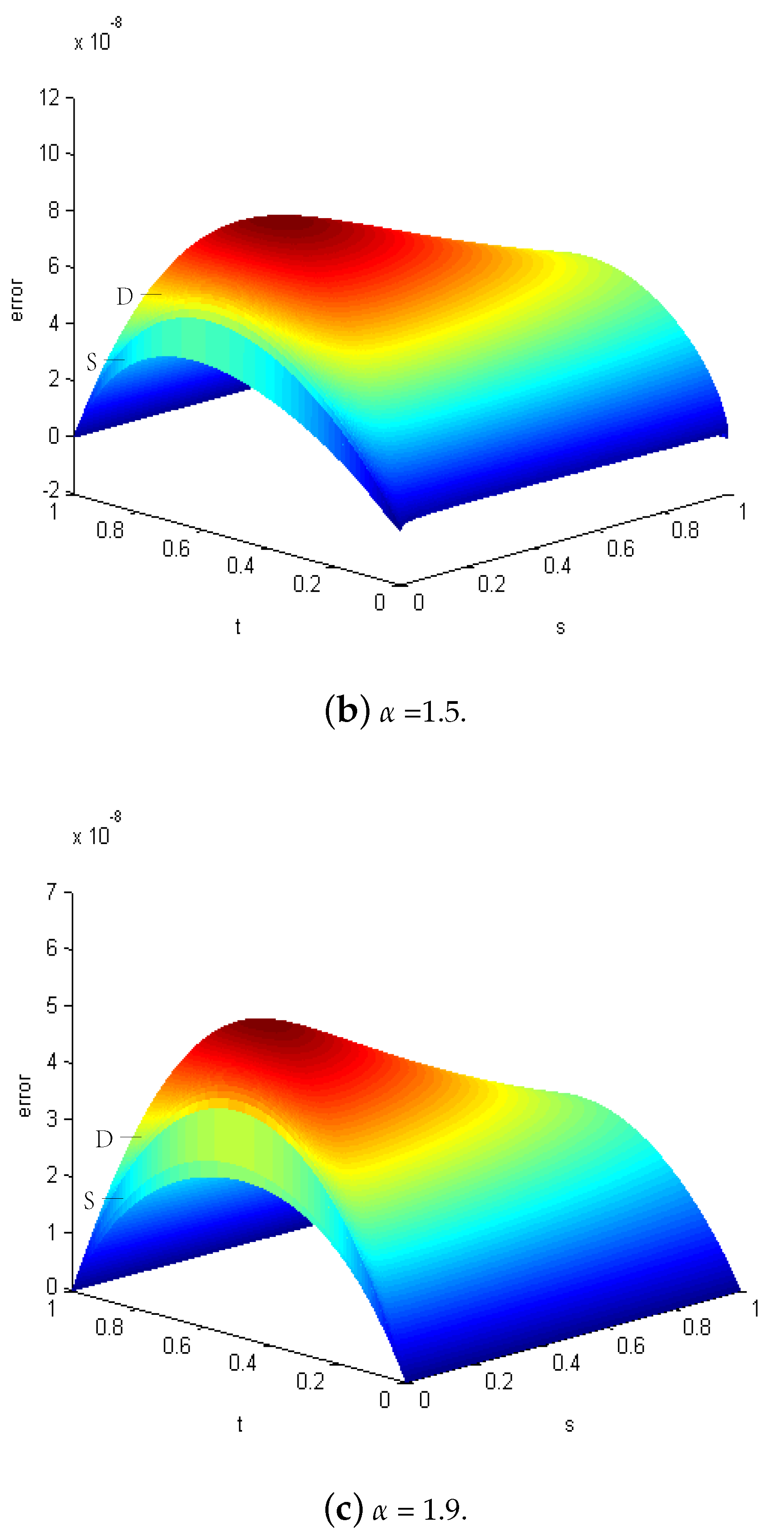
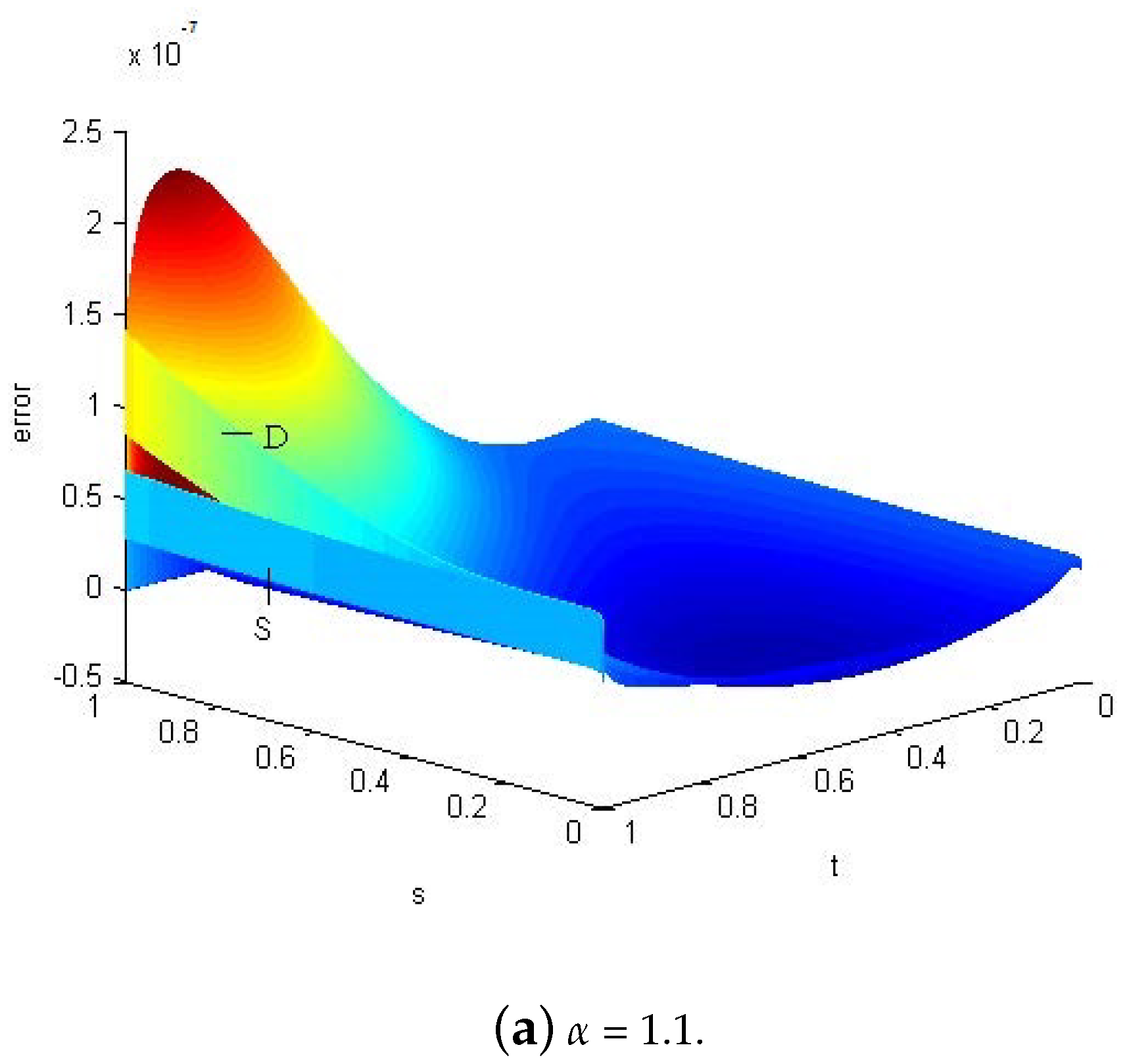
We also carried out further numerical experiments to validate the efficacy of our DS method, with the aim of comparing the error surfaces of the DS and ST methods, and observe any differences in their respective performances. Figure 1 presents the results of our experiments. The figure displays the error surfaces of the DS and ST methods, labeled as “D” and “S” respectively, at specific values of γ = 0.3 and n s = 2048 . The variables t and s in Figure 1 represent the discretized temporal and spatial values, respectively, within the interval [0, 1] in the error functions. Our analysis of the figure revealed that the error surface of the DS method encompasses that of the ST method, but the errors for both methods are at the level of O ( 10 8 ) , which is a relatively low level of error. This result reinforces the effectiveness and reliability of our proposed DS method.
We subsequently increase the value of γ for different α and compare the numerical performance of the DS method with that of the ST method. The obtained results are listed in Table 2. We can see that for different α , the DS method requires 6 iterations to reach the prescribed residual level. For middle-scale problems ( n s = 2048 , 4098 ), the ST method is faster than the DS method in terms of CPU time. However, with increasing scale (from n s = 8192 to 32,768), the DS method gradually becomes faster than the ST method, albeit sacrificing some accuracy. In particular, at the scale of n s = 32,768, the DS method takes only about 1/14 of the CPU time required by the ST method to obtain a solution of the order O ( 10 10 ) , indicating that the DS method is more suitable for dealing with large-scale problems. Furthermore, we conducted numerical experiments with a value of γ = 0.9 . The results, as shown in Table 3, indicate that while the DS method may sacrifice some accuracy, it still outperforms the ST method in terms of CPU time when n s is no less than 8192.
Example 2.
Consider the GFDE (1) with the diffusion coefficient κ = 5 and the weight function λ ( t ) = e b t with b 0 [11]. The source term is
f ( x , t ) = 10 t 3 γ e b t Γ ( 4 γ ) x 2 ( 1 x ) 2 25 g ( t ) { Γ ( 3 ) Γ ( 3 α ) [ p x 2 α + ( 1 p ) ( 1 x ) 2 α ] 2 Γ ( 4 ) Γ ( 4 α ) [ p x 3 α + ( 1 p ) ( 1 x ) 3 α ] + Γ ( 5 ) Γ ( 5 α ) [ p x 4 α + ( 1 p ) ( 1 x ) 4 α ] } .
The corresponding initial-boundary value conditions are u ( x , 0 ) = 5 g ( 0 ) x 2 ( 1 x ) 2 , u ( 0 , t ) = u ( 1 , t ) = 0 . It can be verified that the exact solution function is u ( x , t ) = 5 g ( t ) x 2 ( 1 x ) 2 ( see Appendix A) with
g ( t ) = 1 + 2 ( 2 + 2 b t + b 2 t 2 ) e b t b 3 .
We chose values of p = 0.4 and γ = 0.2 and implemented both algorithms for the discretized Stein equation from Example 2. The results obtained are displayed in Table 4, which demonstrates that both methods are capable of efficiently computing the solution with an error range of approximately between O ( 10 7 ) to O ( 10 9 ) for different values of α . With the exception of when h = 1 / 2048 and α = 1.1 , our DS method required six iterations to achieve the desired residual level. In addition, for α = 1.1 , the DS method was less time-consuming than the ST method but achieved almost the same level of accuracy. For cases where α = 1.5 and 1.9 , our DS method took more CPU time to compute the solution for middle-scale cases where n s was 2048 and 4098. However, as the scale increased, the DS method required less CPU time than the ST method, with only a slight decrease in accuracy.
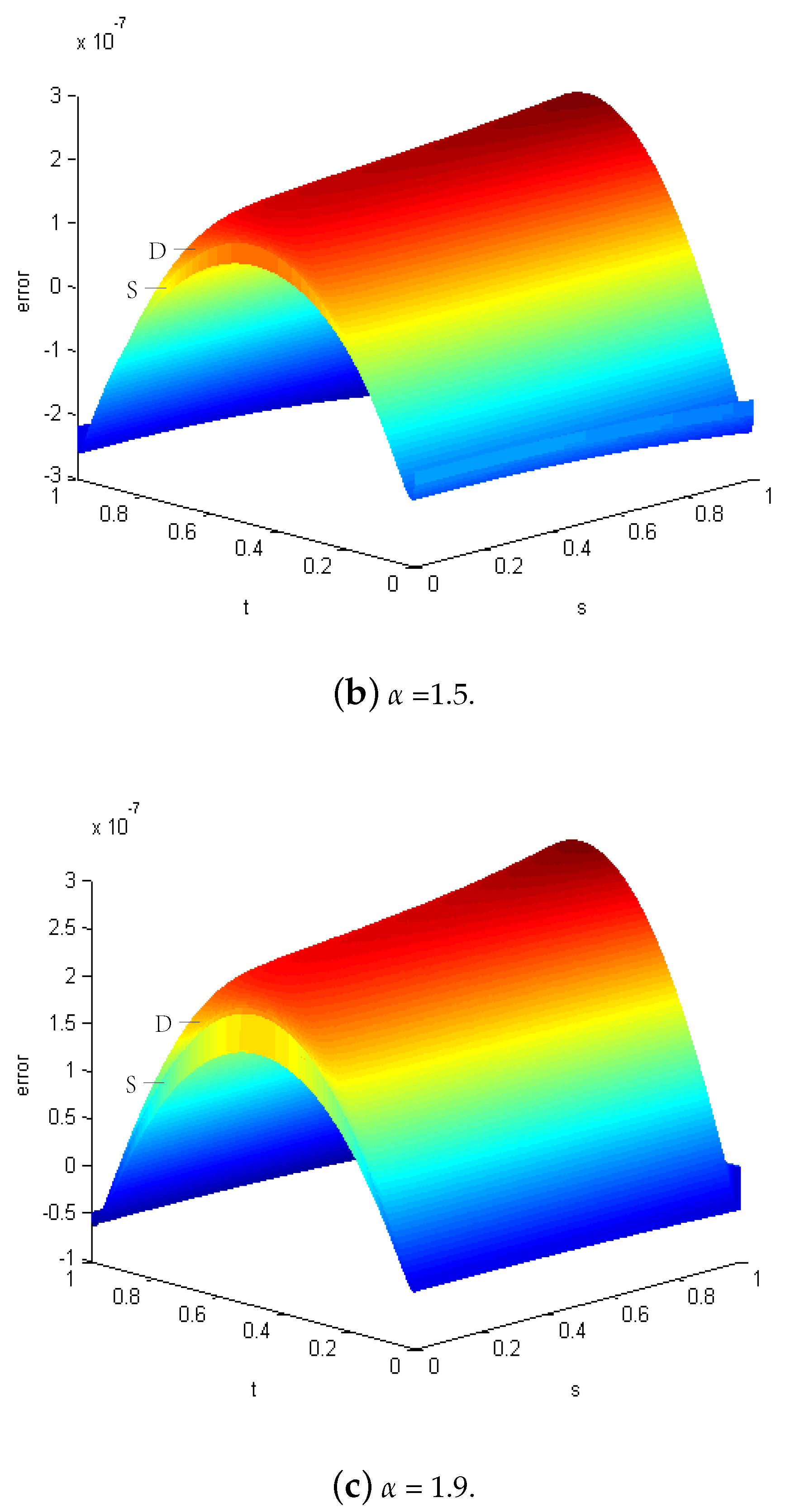
Additionally, we generated error surfaces for both methods and denoted them as “D” for the DS method and “S” for the ST method. These surfaces were plotted at γ = 0.4 and n s = 2048 , and the results are shown in Figure 2. The figure indicates that the error surface of the DS method covers that of the ST method, while both methods have similar error levels of approximately O ( 10 7 ) .
We also raised the parameter γ to 0.5 and executed both algorithms once more. Table 5 illustrates the results, indicating that our DS method produces similar error levels to the ST method. Moreover, when n s = 8192 , our DS method performs better than the ST method in terms of CPU time. This tendency becomes increasingly apparent as the scale increases, demonstrating that the complexity of the DS method is roughly O ( ( n s 1 ) log ( n s 1 ) ) and that it is more suitable for larger-scale problems. In Table 6, we resumed conducting numerical experiments with γ = 0.9 and similarly found that while the DS method may compromise some accuracy, it still outperforms the ST method in terms of CPU time when n s > 8192 .

5. Conclusions

We have presented a doubling Smith iteration method for solving discretized Stein equations arising from a class of generalized fractional diffusion equations (GFDEs). The method takes advantage of the implicit difference scheme, resulting in coefficient matrices with nonsingular M-matrix structures. The two optimal parameters are then determined based on this property, and the separable forcing term of the GFDE contributes to the low-ranked version of the doubling Smith method. Numerical experiments demonstrate that our method outperforms the ST method with the Bi-CGSTAB solver in terms of CPU time, particularly as the scale increases, although it sacrifices some accuracy. However, our approach is limited to GFDEs with the case of λ ( t ) = 1 . It may not be appropriate for solving other types of fractional diffusion equations. Additionally, if the coefficient matrices do not have nonsingular M-matrix structures, the optimal parameters in the presented doubling Smith method may not be determined. As future work, we plan to explore the applicability of the low-ranked doubling Smith methods for solving other large-scale GFDEs. In addition, it should be noted that the GFDE discussed in this paper is limited to zero boundary conditions. It is important to acknowledge that previous studies have shown that the shifted Grunwald–Letnikov formula requires modification when dealing with absorbing boundary conditions. Researchers have explored this area in depth, as evidenced by works such as [27,28,29]. As such, it would be beneficial for future research to focus on extending the technique of the classical method of manufactured solutions [30,31,32,33] to convert non-zero boundary conditions into zero ones. This would allow the GFDE to be applied to a wider range of problems, improving its practicality and usefulness in real-world scenarios.

Author Contributions

Conceptualization, B.Y.; methodology, B.Y.; software, X.L.; validation, N.D.; and formal analysis, X.L. All authors have read and agreed to the final version of this manuscript.

Funding

This work was supported partly by the NSF of Hunan Province (2021JJ50032, 2023JJ50040) and the foundation of Education Department of Hunan Province (HNJG-2021-0129).

Acknowledgments

We are grateful to the academic editor and three anonymous referees for their useful comments and suggestions, which have significantly enhanced the quality the original paper.

Conflicts of Interest

The authors declare no conflict of interest.

Appendix A. Validation of True Solutions in Example 1 and 2

Example A1.
For the solution u ( x , t ) = e t x 3 ( 1 x ) , the γ-order generalized Caputo fractional derivative on the left of GFDE (1) is
0 C D t γ , λ ( t ) u ( x , t ) = 1 Γ ( 1 γ ) 0 t λ ( t η ) ( t η ) γ u ( x , η ) η d η = 1 Γ ( 1 γ ) 0 t e ( t η ) ( t η ) γ e η x 3 ( 1 x ) d η = t 1 γ e t Γ ( 2 γ ) x 3 ( 1 x ) .
The α -order Riemann–Liouville (R-L) fractional derivative on the right of GFDE (1) is
0 D x α u ( x , t ) = 1 Γ ( 2 α ) 2 x 2 0 x u ( ξ , t ) ( x ξ ) α 1 d ξ = e t Γ ( 2 α ) 2 x 2 0 x ξ 3 ξ 4 ( x ξ ) α 1 d ξ = e t Γ ( 2 α ) 2 x 2 ( 6 Π i = 2 5 ( i α ) x 5 α 24 Π i = 2 6 ( i α ) x 6 α ) = 6 e t Γ ( 4 α ) x 3 α 24 e t Γ ( 5 α ) x 4 α .
Then, the GFDE (1) with κ = 1 , p = 1 , and λ ( t ) = e t holds true when the forcing function is
f ( x , t ) = t 1 γ e t Γ ( 2 γ ) x 3 ( 1 x ) 6 e t Γ ( 4 α ) x 3 α + 24 e t Γ ( 5 α ) x 4 α .
Example A2.
For the solution function u ( x , t ) = 5 g ( t ) x 2 ( 1 x ) 2 , the γ-order generalized Caputo fractional derivative on the left of GFDE (1) is
0 C D t γ , λ ( t ) u ( x , t ) = 1 Γ ( 1 γ ) 0 t λ ( t η ) ( t η ) γ u ( x , η ) η d η = 1 Γ ( 1 γ ) 0 t ( t η ) γ e b ( t η ) [ 5 x 2 ( 1 x ) 2 η 2 e b η ] d η = 10 t 3 γ e b t Γ ( 4 γ ) x 2 ( 1 x ) 2 .
The α -order Riemann–Liouville (R-L) fractional derivatives on the right of GFDE (1) are
0 D x α u ( x , t ) = 1 Γ ( 2 α ) 2 x 2 0 x u ( ξ , t ) ( x ξ ) α 1 d ξ = 5 g ( t ) Γ ( 2 α ) 2 x 2 0 x ξ 2 ( 1 ξ ) 2 ( x ξ ) α 1 d ξ = 5 g ( t ) Γ ( 2 α ) 2 x 2 ( 2 Π i = 2 4 ( i α ) x 4 α 12 Π i = 2 5 ( i α ) x 5 α + 24 Π i = 2 6 ( i α ) x 6 α ) = 5 g ( t ) [ Γ ( 3 ) Γ ( 3 α ) x 2 α 2 Γ ( 4 ) Γ ( 4 α ) x 3 α + Γ ( 5 ) Γ ( 5 α ) x 4 α ]
and
x D 1 α u ( x , t ) = 1 Γ ( 2 α ) 2 x 2 x 1 u ( ξ , t ) ( ξ x ) α 1 d ξ = 5 g ( t ) Γ ( 2 α ) 2 x 2 x 1 ξ 2 ( 1 ξ ) 2 ( ξ x ) α 1 d ξ = 5 g ( t ) Γ ( 2 α ) 2 x 2 ( 2 Π i = 2 4 ( i α ) ( 1 x ) 4 α 12 Π i = 2 5 ( i α ) ( 1 x ) 5 α + 24 Π i = 2 6 ( i α ) ( 1 x ) 6 α ) = 5 g ( t ) [ Γ ( 3 ) Γ ( 3 α ) ( 1 x ) 2 α 2 Γ ( 4 ) Γ ( 4 α ) ( 1 x ) 3 α + Γ ( 5 ) Γ ( 5 α ) ( 1 x ) 4 α ] .
Then, the GFDE (1) with κ = 5 and λ ( t ) = e b t holds true when the forcing function is
f ( x , t ) = 10 t 3 γ e b t Γ ( 4 γ ) x 2 ( 1 x ) 2 25 g ( t ) { Γ ( 3 ) Γ ( 3 α ) [ p x 2 α + ( 1 p ) ( 1 x ) 2 α ] 2 Γ ( 4 ) Γ ( 4 α ) [ p x 3 α + ( 1 p ) ( 1 x ) 3 α ] + Γ ( 5 ) Γ ( 5 α ) [ p x 4 α + ( 1 p ) ( 1 x ) 4 α ] } .

References

  1. Alikhanov, A.A. A time-fractional diffusion equation with generalized memory kernel in differential and difference settings with smooth solutions. Comput. Methods Appl. Math. 2017, 17, 647–660. [Google Scholar] [CrossRef]
  2. Sandev, T.; Chechkin, A.; Kantz, H.; Metzler, R. Diffusion and Fokker-Planck-Smoluchowski equations with generalized memory kernel. Fract. Calc. Appl. Anal. 2015, 18, 1006–1038. [Google Scholar] [CrossRef]
  3. Santos, M.A.F. Mittag-Leffler memory kernel in Lévy flights. Mathematics 2019, 7, 766. [Google Scholar] [CrossRef]
  4. Chen, M.; Deng, W. High order algorithm for the time-tempered fractional Feynman-Kac equation. J. Sci. Comput. 2018, 76, 867–887. [Google Scholar] [CrossRef]
  5. Wu, X.; Deng, W.; Barkai, E. Tempered fractional Feynman-Kac equation: Theory and examples. Phys. Rev. E 2016, 93, 032151. [Google Scholar] [CrossRef]
  6. Kostić, M. Abstract Volterra Integro-Differential Equations; CRC Press: Boca Raton, FL, USA, 2015. [Google Scholar]
  7. Lin, F.-R.; Yang, S.-W.; Jin, X.-Q. Preconditioned iterative methods for fractional diffusion equation. J. Comput. Phys. 2014, 256, 109–117. [Google Scholar] [CrossRef]
  8. Meerschaert, M.M.; Tadjeran, C. Finite difference approximations for two-sided space-fractional partial differential equations. Appl. Numer. Math. 2006, 56, 80–90. [Google Scholar] [CrossRef]
  9. Bazhlekova, E. Fractional Evolution Equations in Banach Spaces. Ph.D. Thesis, Eindhoven University of Technology, Eindhoven, The Netherlands, 2001. [Google Scholar]
  10. Tadjeran, C.; Meerschaert, M.M.; Scheffler, H.-P. A second-order accurate numerical approximation for the fractional diffusion equation. J. Comput. Phys. 2006, 213, 205–213. [Google Scholar] [CrossRef]
  11. Gu, X.-M.; Huang, T.-Z.; Zhao, Y.-L.; Lyu, P.; Carpentieri, B. A fast implicit difference scheme for solving the generalized time-space fractional diffusion equations with variable coefficients. Numer. Meth. Part. Differ. Equ. 2021, 37, 1136–1162. [Google Scholar] [CrossRef]
  12. Podlubny, I. Fractional differential Equations, Mathematics in Science; Academic Press: San Diego, CA, USA, 1999. [Google Scholar]
  13. Pitolli, F.; Sorgentone, C.; Pellegrino, E. Approximation of the Riesz–Caputo Derivative by Cubic Splines. Algorithms 2022, 15, 69. [Google Scholar] [CrossRef]
  14. Shymanskyi, V.; Sokolovskyy, T. Finite element calculation of the linear elasticity problem for biomaterials with fractal structure. Open Bioinform. J. 2021, 14 (Suppl. M1), 114–122. [Google Scholar] [CrossRef]
  15. Izadi, M.; Srivastava, H.M. A Discretization Approach for the Nonlinear Fractional Logistic Equation. Entropy 2020, 22, 1328. [Google Scholar] [CrossRef]
  16. Li, T.-X.; Weng, P.C.-Y.; Chu, E.K.-W.; Lin, W.-W. Large-scale Stein and Lyapunov equtions, Smith method, and applications. Numer. Algorithms 2013, 63, 727–752. [Google Scholar] [CrossRef]
  17. Yu, B.; Fan, H.-Y.; Chu, E.K.-W. Smith method for projected Lyapunov and Stein equations. Univ. Politeh. Buchar. Sci. Bull.-Ser. A-Appl. Math. Phys. 2018, 80, 191–204. [Google Scholar]
  18. Kelly, C.T. Iterative Methods for Linear and Nonlinear Equations; SIAM: Philadelphia, PA, USA, 1995. [Google Scholar]
  19. Varga, R. Matrix Iterative Analysis, 2nd ed.; Springer: Berlin/Heidelberg, Germeny, 2000. [Google Scholar]
  20. Wang, W.-G.; Wang, W.-C.; Li, R.-C. Alternating-directional doubling algorithm for M-matrix algebraic Riccati equations. SIAM J. Matrix Anal. Appl. 2012, 33, 170–194. [Google Scholar] [CrossRef]
  21. Gu, X.-M.; Huang, T.-Z.; Ji, C.-C.; Carpentieri, B.; Alikhanov, A.A. Fast iterative method with a second-order implicit difference scheme for time-space fractional convection-diffusion equation. J. Sci. Comput. 2017, 72, 957–985. [Google Scholar] [CrossRef]
  22. Hao, Z.-P.; Sun, Z.-Z.; Cao, W.-R. A fourth-order approximation of fractional derivatives with its applications. J. Comput. Phys. 2015, 281, 787–805. [Google Scholar] [CrossRef]
  23. Tian, W.-Y.; Zhou, H.; Deng, W.-H. A class of second order difference approsimation for solving space fractional diffusion equations. Math. Comput. 2015, 84, 1703–1727. [Google Scholar] [CrossRef]
  24. Ng, M. Iterative Methods for Toeplitz Systems; Oxford University Press: New York, NY, USA, 2004. [Google Scholar]
  25. Chu, E.K.-W.; Weng, P.C.-Y. Large-scale discrete-time algebraic Riccati equations—Doubling algorithm and error analysis. J. Comput. Appl. Math. 2015, 277, 115–126. [Google Scholar] [CrossRef]
  26. Gohberg, I.; Semencul, A. On the inversion of finite Toeplitz matrices and their continuous analogues. Mat. Issled. 1972, 7, 201–223. (In Russian) [Google Scholar]
  27. Kelly, F.; Sankaranarayanan, H.; Meerschaert, M. Boundary conditions for two-sided fractional diffusion. J. Comput. Phys. 2019, 376, 1089–1107. [Google Scholar] [CrossRef]
  28. Krepysheva, N.; Di Pietro, L.; Néel, C. Space-fractional advection-diffusion and reflective boundary condition. Phys. Rev. E 2006, 73, 021104. [Google Scholar] [CrossRef]
  29. Baeumer, B.; Kovács, M.; Meerschaert, M.; Sankaranarayanan, H. Reprint of: Boundary conditions for fractional diffusion. J. Comput. Appl. Math. 2018, 339, 414–430. [Google Scholar] [CrossRef]
  30. Tremblay, D.; Stephane, E.; Dominique, P. Code verification and the method of manufactured solutions for fluid-structure interaction problems. In Proceedings of the 36th AIAA Fluid Dynamics Conference and Exhibit, San Francisco, CA, USA, 5–8 June 2006. [Google Scholar]
  31. Krueger, M.; Mousseau, A.; Hassan, A. Rigorous code verification: An additional tool to use with the method of manufactured solutions. In Verification and Validation; American Society of Mechanical Engineers: New York, NY, USA, 2019; Volume 41174, p. V001T04A002. [Google Scholar]
  32. Vedovoto, J.M.; da Silveira, N.A.; Mura, A.; da Silva, L.F.F. Application of the method of manufactured solutions to the verification of a pressure-based finite-volume numerical scheme. Comput. Fluids 2011, 51, 85–99. [Google Scholar] [CrossRef]
  33. Shunn, L.; Ham, F. Method of manufactured solutions applied to variable-density flow solvers. In Annual Research Briefs-2007; Center for Turbulence Research: San Francisco, CA, USA, 2007; pp. 155–168. [Google Scholar]
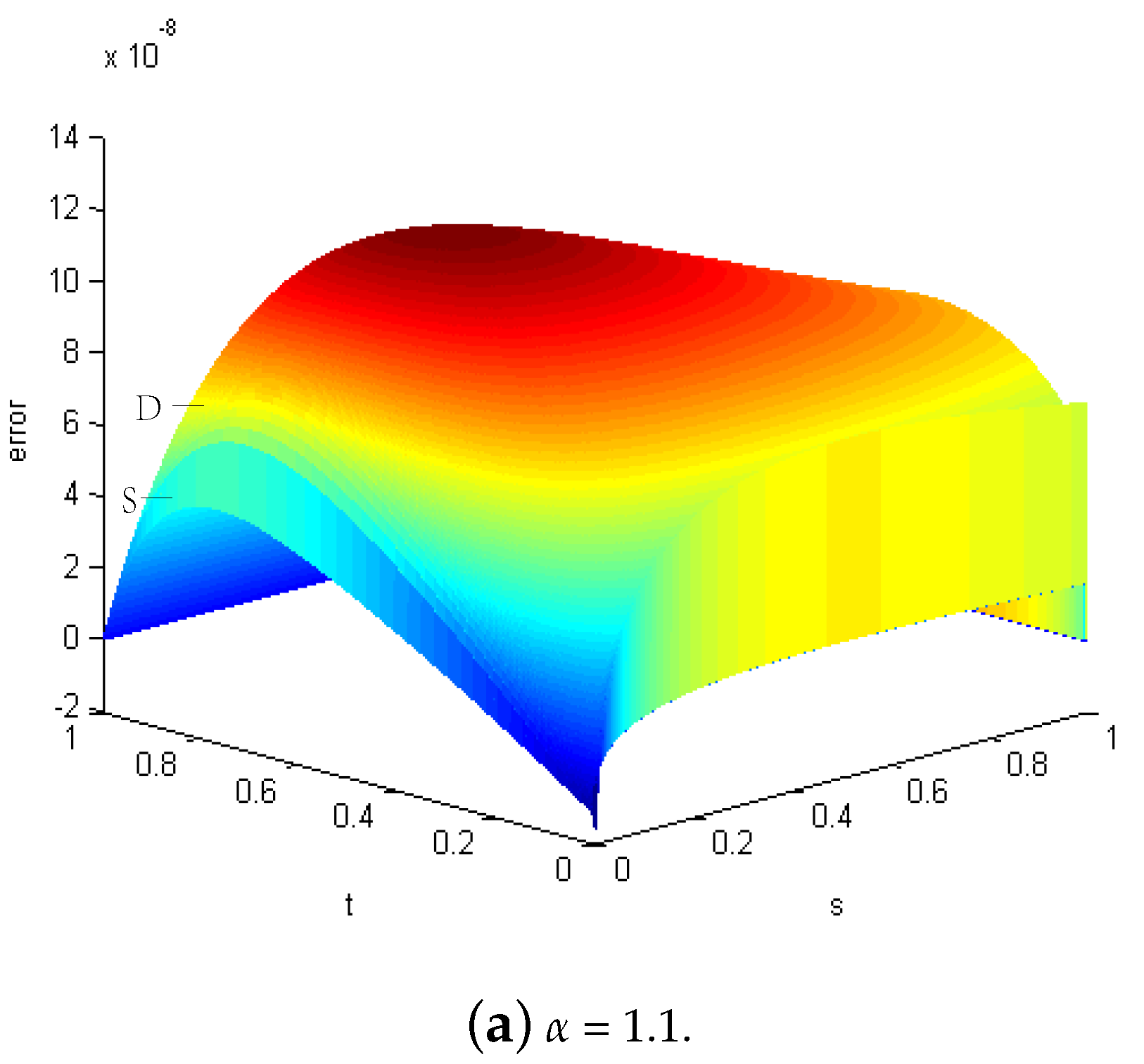
Figure 1. Error surfaces calculated by the DS method (D) and the ST method (S) at n s = 2048 and γ = 0.3 in Example 1. The subplots from top to bottom correspond to different α .
Fractalfract 07 00380 g001aFractalfract 07 00380 g001b
Figure 2. Error surfaces calculated by the DS method (D) and the ST method (S) at n s = 2048 and γ = 0.4 in Example 2. The subplots from top to bottom correspond to different α .
Fractalfract 07 00380 g002aFractalfract 07 00380 g002b
Table 1. Numerical performances of two different methods when γ = 0.2 in Example 1.
γ = 0.2 hCPU_STCPU_DS (It.)Rate_DSErr_STErr_DS
1/20484.272.31 (5)1.38 ×   10 7 1.38 ×   10 7
1/409617.003.83 (5)2.0053.44 ×   10 8 3.44 ×   10 8
α = 1.1 1/8192116.528.02 (5)2.0068.57 ×   10 9 8.57 ×   10 9
1/16,384792.3015.54 (6)2.0082.13 ×   10 9 2.13 ×   10 9
1/32,7685805.97111.84 (6)2.0045.31 ×   10 10 5.31 ×   10 10
1/20484.322.34 (5)9.71 ×   10 8 9.71 ×   10 8
1/409616.623.79 (5)2.0052.42 ×   10 8 2.42 ×   10 8
α = 1.5 1/8192120.038.19 (5)2.1336.03 ×   10 9 5.52 ×   10 9
1/16,384789.3115.55 (5)2.0051.30 ×   10 9 1.37 ×   10 9
1/32,7685830.8638.36 (5)1.1863.64 ×   10 10 6.02 ×   10 10
1/20484.280.73 (4)5.81 ×   10 8 5.62 ×   10 8
1/409615.933.57 (4)2.0011.45 ×   10 8 1.41 ×   10 8
α = 1.9 1/8192117.388.04(5)1.8273.62 ×   10 9 3.96 ×   10 9
1/16,384786.5715.12 (5)1.2818.41 ×   10 10 1.71 ×   10 9
1/32,7685838.16431.24 (6)1.0392.95 ×   10 10 8.32 ×   10 10
Table 2. Numerical performances of two different methods when γ = 0.5 in Example 1.
γ = 0.5 hCPU_STCPU_DS (It.)Rate_DSErr_STErr_DS
1/20484.1425.21(6)7.48 ×   10 8 7.52 ×   10 8
1/409615.8842.74 (6)2.0231.33 ×   10 8 1.85 ×   10 7
α = 1.1 1/8192117.3399.25 (6)2.0882.24 ×   10 9 4.35 ×   10 9
1/16,384803.19197.31 (6)1.9576.27 ×   10 10 1.12 ×   10 9
1/32,7685568.40420.32 (6)1.5592.02 ×   10 10 3.80 ×   10 10
1/20485.1424.69 (6)5.96 ×   10 8 6.13 ×   10 8
1/409616.1243.80 (6)2.1201.17 ×   10 8 1.41 ×   10 8
α = 1.5 1/8192117.7898.53 (6)2.0101.83 ×   10 9 3.50 ×   10 9
1/16,384798.62198.50 (6)1.8451.27 ×   10 10 9.74 ×   10 10
1/32,7685584.45420.80 (6)1.6333.11 ×   10 11 3.14 ×   10 10
1/20486.3929.16 (6)3.83 ×   10 8 3.96 ×   10 8
1/409616.3644.39 (6)2.1508.00 ×   10 9 8.92 ×   10 9
α = 1.9 1/8192118.9699.52 (6)2.0661.31 ×   10 9 2.13 ×   10 9
1/16,384792.86194.41 (6)1.1155.71 ×   10 10 9.83 ×   10 10
1/32,7685544.37429.55 (6)0.9169.34 ×   10 11 5.21 ×   10 10
Table 3. Numerical performances of two different methods when γ = 0.9 in Example 1.
γ = 0.9 hCPU_STCPU_DS (It.)Rate_DSErr_STErr_DS
1/20484.7225.73(6)2.34 ×   10 6 9.64 ×   10 6
1/409616.4945.68 (6)1.0721.12 ×   10 6 4.75 ×   10 6
α = 1.1 1/8192125.95112.17 (6)0.9115.32 ×   10 7 2.43 ×   10 6
1/16,384857.63226.60 (6)1.0292.50 ×   10 7 1.19 ×   10 6
1/32,7685416.31405.57 (6)0.5231.05 ×   10 7 8.30 ×   10 7
1/20485.0329.10 (6)1.16 ×   10 6 9.84 ×   10 6
1/409620.5545.28 (6)0.9225.61 ×   10 7 5.19 ×   10 6
α = 1.5 1/8192122.46100.14 (6)0.8052.67 ×   10 7 2.97 ×   10 6
1/16,384802.23196.10 (6)1.1371.26 ×   10 7 1.35 ×   10 6
1/32,7685496.12428.64 (6)0.5379.42 ×   10 8 9.32 ×   10 7
1/20484.3224.58 (6)6.31 ×   10 7 4.26 ×   10 6
1/409616.3642.56 (6)0.6963.06 ×   10 7 2.63 ×   10 6
α = 1.9 1/8192121.8398.89 (6)0.7721.46 ×   10 7 1.54 ×   10 7
1/16,384803.47194.59 (6)0.8746.91 ×   10 8 8.42 ×   10 7
1/32,7685521.86435.56 (6)0.5734.75 ×   10 8 5.66 ×   10 7
Table 4. Numerical performances of two different methods when γ = 0.2 , p = 0.4 in Example 2.
γ = 0.2 , p = 0.4 hCPU_STCPU_DS (It.)Rate_DSErr_STErr_DS
1/20484.432.23 (5)6.59 ×   10 7 6.59 ×   10 7
1/409616.6214.57 (6)1.98721.66 ×   10 7 1.66 ×   10 7
α = 1.1 1/8192121.8532.28 (6)1.99124.16 ×   10 8 4.16 ×   10 8
1/16,384779.2764.17 (6)1.99381.04 ×   10 8 1.04 ×   10 8
1/32,7685579.25521.88 (6)1.99562.62 ×   10 9 2.62 ×   10 9
1/20484.1623.58 (6)2.99 ×   10 7 2.99 ×   10 7
1/409615.8644.47 (6)1.99297.76 ×   10 8 7.75 ×   10 8
α = 1.5 1/8192127.21103.13 (6)1.76472.00 ×   10 8 2.28 ×   10 8
1/16,384791.21221.25 (6)1.37605.14 ×   10 9 8.78 ×   10 9
1/32,7685742.21532.20 (6)1.18161.31 ×   10 9 3.86 ×   10 9
1/20486.1419.69 (6)2.94 ×   10 7 2.94 ×   10 7
1/409616.7237.14 (6)1.95827.23 ×   10 8 7.53 ×   10 8
α = 1.9 1/8192120.8383.25 (6)1.86301.83 ×   10 8 2.07 ×   10 8
1/16,384795.98169.03 (6)1.42102.94 ×   10 9 5.73 ×   10 9
1/32,7685813.56478.80 (6)0.49611.05 ×   10 9 4.07 ×   10 9
Table 5. Numerical performances of two different methods when γ = 0.5 , p = 0.4 in Example 2.
γ = 0.5 , p = 0.4 hCPU_STCPU_DS (It.)Rate_DSErr_STErr_DS
1/20484.4130.12 (6)6.41 ×   10 7 6.41 ×   10 7
1/409616.8255.45 (6)1.95791.60 ×   10 7 1.65 ×   10 7
α = 1.1 1/8192122.68111.99 (6)1.86524.00 ×   10 8 4.53 ×   10 8
1/16,384739.46246.17 (6)1.82349.95 ×   10 9 1.28 ×   10 8
1/32,7685954.71520.47 (6)1.75972.47 ×   10 9 3.78 ×   10 9
1/20484.1628.98 (6)2.98 ×   10 7 2.98 ×   10 7
1/409615.7755.01 (6)1.94287.72 ×   10 8 7.76 ×   10 8
α = 1.5 1/8192117.98101.78 (6)1.84481.99 ×   10 8 2.16 ×   10 8
1/16,384785.39246.42 (6)1.56905.10 ×   10 9 7.28 ×   10 9
1/32,7685744.93536.89.26 (6)1.57211.29 ×   10 9 2.45 ×   10 9
1/20484.3829.96 (6)3.01 ×   10 7 3.01 ×   10 7
1/409616.7455.44 (6)2.0057.46 ×   10 8 7.53 ×   10 8
α = 1.9 1/8192118.82103.35 (6)1.84231.89 ×   10 8 2.10 ×   10 8
1/16,384810.04246.57 (6)1.30304.14 ×   10 9 8.53 ×   10 9
1/32,7685816.90550.72 (6)0.00511.96 ×   10 9 8.50 ×   10 9
Table 6. Numerical performances of two different methods when γ = 0.9 , p = 0.4 in Example 2.
γ = 0.9 , p = 0.4 hCPU_STCPU_DS (It.)Rate_DSErr_STErr_DS
1/20484.5329.75 (6)3.78 ×   10 6 4.08 ×   10 6
1/409617.2954.29 (6)1.02131.72 ×   10 6 2.01 ×   10 6
α = 1.1 1/8192126.29128.06 (6)0.93687.94 ×   10 7 1.05 ×   10 6
1/16,384814.66243.67 (6)0.71243.68 ×   10 7 6.42 ×   10 7
1/32,7686043.21518.66 (6)0.62251.53 ×   10 7 4.17 ×   10 7
1/20484.3129.78 (6)9.72 ×   10 7 1.23 ×   10 6
1/409616.4554.31 (6)1.01054.07 ×   10 7 6.12 ×   10 7
α = 1.5 1/8192122.19124.77 (6)0.74161.79 ×   10 7 3.66 ×   10 7
1/16,384802.35243.98 (6)0.89368.06 ×   10 8 1.97 ×   10 7
1/32,7685804.55522.53 (6)0.99703.90 ×   10 8 9.88 ×   10 8
1/20484.5229.63 (6)5.79 ×   10 7 9.54 ×   10 7
1/409617.4454.40 (6)1.01212.11 ×   10 7 4.73 ×   10 7
α = 1.9 1/8192124.43123.46 (6)0.64258.37 ×   10 8 3.03 ×   10 7
1/16,384810.55244.26 (6)0.85083.46 ×   10 8 1.68 ×   10 7
1/32,7685978.33562.76 (6)0.59791.41 ×   10 8 1.11 ×   10 7
Disclaimer/Publisher’s Note: The statements, opinions and data contained in all publications are solely those of the individual author(s) and contributor(s) and not of MDPI and/or the editor(s). MDPI and/or the editor(s) disclaim responsibility for any injury to people or property resulting from any ideas, methods, instructions or products referred to in the content.