Article

Laplace-Residual Power Series Method for Solving Time-Fractional Reaction–Diffusion Model

1
Department of Mathematics, Faculty of Science, Al Balqa Applied University, Salt 19117, Jordan
2
Department of Basic Sciences, Faculty of Arts and Sciences, Al-Ahliyyah Amman University, Amman 19328, Jordan
3
Mathematics Department, Al-Qunfudah University College, Umm Al-Qura University, Mecca 24382, Saudi Arabia
*
Author to whom correspondence should be addressed.
Fractal Fract. 2023, 7(4), 309; https://doi.org/10.3390/fractalfract7040309
Submission received: 19 January 2023 / Revised: 11 February 2023 / Accepted: 23 February 2023 / Published: 2 April 2023

Abstract

:
Despite the fact the Laplace transform has an appreciable efficiency in solving many equations, it cannot be employed to nonlinear equations of any type. This paper presents a modern technique for employing the Laplace transform LT in solving the nonlinear time-fractional reaction–diffusion model. The new approach is called the Laplace-residual power series method (L-RPSM), which imitates the residual power series method in determining the coefficients of the series solution. The proposed method is also adapted to find an approximate series solution that converges to the exact solution of the nonlinear time-fractional reaction–diffusion equations. In addition, the method has been applied to many examples, and the findings are found to be impressive. Further, the results indicate that the L-RPSM is effective, fast, and easy to reach the exact solution of the equations. Furthermore, several actual and approximate solutions are graphically represented to demonstrate the efficiency and accuracy of the proposed method.

1. Introduction

Fractional integral and derivatives are a branch of applied mathematical analysis and have been developed theoretically in recent years [1,2,3,4,5,6,7,8,9,10,11]; the application of this field has been used in many areas such as sciences, engineering, aerodynamic, thermodynamic, mechatronics, image processing, physics, and fluid flow phenomena [12,13]. The essential improvement of fractional differential equations (FDEs) is to provide a tool for the definition of different behaviors in different fields.
Most FDEs do not have exact analytic solutions, so approximation methods (numerical or analytical) must be used, such as the Jacobi Tau method [14], the Sinc–Legendre collocation method [15], the Petrov–Galerkin algorithm [16], the decomposition method [8,17], the Variational iteration method [18], and the homotopy transformation perturbation method [19]. The RPSM is an effective method used to solve wide classes of differential equations [20].
Eriqat et al. [21] proposed a new scheme to solve a class of fractional differential equations by combining the LT and the RPSM and called it the L-RPSM. This new method is guaranteed to have more simplicity than RPSM for creating the exact and approximate solutions (ASs) to the linear and nonlinear FDEs, such as the neutral FDEs [21], the nonlinear time-dispersive fractional partial differential equations (FPDEs) [22], the nonlinear fractional reaction–diffusion for bacteria growth model [23], the time-fractional nonlinear fisher PDE [24], the fuzzy fractional population dynamics model [25], the fuzzy quadratic Riccati differential equations [26], the fractional Lane-Emden equations [27], and the high-order FPDEs [28].
The reaction–diffusion equations describe the behavior of a large range of chemical systems where the diffusion of material competes with the production of that material by some form of chemical reaction. The simplest reaction–diffusion models are of the form [29]:
D t ν = M ( x ) D x 2 ν + r ( ν ) ,
where ν = ν ( x , t ) , M ( x ) is a continous function, x R , t > 0 , and r ( ν ) is a non-linear analytic function of ν that is chosen as reaction kinetics.
Recently, Equation (1) has been reformulated by replacing the time-first derivative with a time-fractional derivative, so it becomes as follows [19,30,31]:
D t α ν = M ( x ) D x 2 ν + r ( ν ) ,
where α ( 0 < α 1 ) is a parameter defining the time Caputo fractional derivative (C-FD) order.
Several researchers have used different methods to solve the non-linear time-fractional reaction diffusion equation (TFRDE) in Equation (2), such as Elzaki homotopy transformation perturbation method [19], the RPSM method [31], the homotopy analysis method [30], and other methods [32,33,34,35,36,37,38,39].
In this paper, the L-RPSM is modified and adapted to create a series solution for the TFRDE, and comparisons with previous methods are made to show the ease and efficiency of the technique. Solving TFRDE using the L-RPSM consists of three steps: (i) convert the given TFRDE into Laplace space, (ii) construct a series solution to the Laplace form of TFRDE, and (iii) convert the solution to the original space using the inverse LT. The L-RPSM introduces a new nice fractional expansion that is used to find the coefficients of a series solution without using fractional derivatives as in RPSM. Additionally, a few simple calculations give us the coefficients of a series compared to the RPSM, which requires several calculations to establish the fractional derivatives in the solution steps. Finally, the exact and accurate approximation solutions by L-RPSM can be obtained with a rapidly convergent series.
The paper is organized as follows: Section 2 reviews some important results related to C-FD and LT. In Section 3, we construct the ASs for TFRDE based on our proposed L-RPSM. In Section 4, applications are performed to validate the efficiency and accuracy of the proposed method. Finally, we provided a conclusion in Section 5.

2. C-FD Operator, LT, and Fractional Expansions

This section reviews some important concepts of C-FD and suggests fractional expansion in LT space to construct exact and ASs for the TFRDEs in the next section. For more information about C-FD and LT, the reader can refer to Refs. [1,2,3,4,5,6,21,22].
Definition 1
([1]). The C-FD of v ( x , t ) for order α is given by:
D t α v ( x , t ) = α v ( x , t ) t α = J t m α m v ( x , t ) t m , m 1 < α < m , m v ( x , t ) t m , α = m N ,
where t 0 , x I , I is an interval, D t α refers to the C-FD of order α , m N , and J t β denotes the Riemann–Liouville fractional integral operator of order β that given by:
J t β ν ( x , t ) = 1 Γ ( β ) 0 t ( t τ ) β 1 ν ( x , t ) d τ , β > 0 , t > τ 0 , ν ( x , t ) β = 0 ,
provided the integral exists.
Lemma 1
([1]). For m 1 < α m , γ > α 1 , t 0 , and λ R , we summarize some important properties for C-FD as follows:
1. 
D t α λ = 0 .
2. 
D t α t γ = Γ ( γ + 1 ) Γ ( γ + 1 α ) t γ α .
3. 
D t α J t α ν ( x , t ) = ν ( x , t ) .
4. 
J t α D t α ν ( x , t ) = ν ( x , t ) j = 0 m 1 t j ν ( x , 0 + ) t j j ! .
Definition 2
([40]). Let ν ( x , t ) be a piecewise continuous function (PCF) on I × [ 0 , ) and of exponential order (EO) δ. Then, the LT of the ν ( x , t ) is defined as:
V ( x , s ) = L [ ν ( x , t ) ] : = 0 e s t ν ( x , t ) d t , s > δ ,
and the inverse LT of the V ( x , s ) is defined as:
ν ( x , t ) = L 1 [ V ( x , s ) ] : = c i c + i e s t V ( x , s ) d s , c = R e ( s ) > c 0 ,
where c 0 lies in the right half plane of the absolute convergence of the Laplace integral.
Lemma 2
([40]). Let u ( x , t ) and v ( x , t ) be PCFs on I × [ 0 , ) and of EOs δ 1 and δ 2 , respectively, where δ 1 < δ 2 . Suppose that U ( x , s ) = L [ u ( x , t ) ] ; V ( x , s ) = L [ v ( x , t ) ] ; and a , b are constants. Then,
1. 
L [ a u ( x , t ) + b v ( x , t ) ] = a U ( x , s ) + b V ( x , s ) , x I , s > δ 1 .
2. 
L [ e a t v ( x , t ) ] = V ( x , s a ) , x I , s > a + δ 1 .
3. 
l i m s s V ( x , s ) = v ( x , 0 ) , x I .
Lemma 3
([22]). Let ν ( x , t ) be a PCF on I × [ 0 , ) and of EO δ, V ( x , s ) = L [ ν ( x , t ) ] . Then, the following properties of LT operator for C-FD are satisfied:
1. 
L [ D t α ν ( x , t ) ] = s α V ( x , s ) k = 0 m 1 s α k 1 t k ν ( x , 0 ) , m 1 < α < m .
2. 
L [ D t n α ν ( x , t ) ] = s n α V ( x , s ) k = 0 n 1 s ( n k ) α 1 D t k α ν ( x , 0 ) , 0 < α 1 ,
where D t n α = D t α . D t α D t α (n-times).
Theorem 1
([22]). Let ν ( x , t ) be a PCF on I × [ 0 , ) and of EO δ. If the function V ( x , s ) = L [ ν ( x , t ) ] has a fractional expansion as follows:
V ( x , s ) = n = 0 f n ( x ) s n α + 1 , 0 < α 1 , x I , s > δ ,
then f n ( x ) = D t n α u ( x , 0 ) .
Remark 1
([22]). The inverse LT of the expansion in Theorem 1 has the following form:
ν ( x , t ) = n = 0 D t n α ν ( x , 0 ) Γ ( n α + 1 ) t n α , 0 < α 1 , t 0 .

3. The L-RPSM for Solving TFRDE

In this section, we apply L-RPSM to the nonlinear TFRDE to be discussed.
Step 1. 
Employ LT to both sides of Equation (2), i.e.,
L [ D t α ν ( x , t ) ] = M ( x ) L [ D x 2 ν ( x , t ) ] + L [ r ( ν ( x , t ) ) ]
By the fact (1) in Lemma 3 at α ( 0 , 1 ] , one can rewrite Equation (9) as
V ( x , s ) = ν ( x , 0 ) s + M ( x ) s α D x 2 V ( x , s ) + R x , s s α ,
where V ( x , s ) = L [ ν ( x , t ) ] and R x , s = L [ r ( ν ( x , t ) ) ] .
Step 2. 
Construct a series solution to the Laplace form:
  • Write the series solution, V ( x , s ) of Equation (10) as follows:
    V ( x , s ) = n = 0 f n ( x ) s n α + 1 ,
    and the kth-truncated solution as
    V k ( x , s ) = n = 0 k f n ( x ) s n α + 1 .
    It is noteworthy that the convergence of the series (11) is discussed in detail in Ref. [22].
    We suppose that the initial guess of Equation (2) is ν ( x , 0 ) = f ( x ) . Hence, according to fact (3) in Lemma 2 we have f 0 ( x ) = lim s s V ( x , s ) = ν ( x , 0 ) = f ( x ) . So, Equation (12) can be written as:
    V k ( x , s ) = f ( x ) s + n = 1 k f n ( x ) s n α + 1 .
  • Construct the Laplace-Residual function (LRF), L R e s ( x , s ) , to Equation (10) as:
    L R e s ( x , s ) = V ( x , s ) f ( x ) s M ( x ) s α D x 2 V ( x , s ) R x , s s α ,
    and the kth-LRF, L R e s k ( x , s ) is
    L R e s k ( x , s ) = V k ( x , s ) f ( x ) s M ( x ) s α D x 2 V k ( x , s ) R x , s s α .
  • Substitute the kth-truncation, V k ( x , s ) , as in Equation (13), into Equation (15) and multiply both sides of resulting equation by s k α + 1 , k = 1 , 2 ,
  • To obtain the requited coefficients, f n ( x ) , n = 1 , 2 , , k , in Equation (13), we solve the following algebraic equation recursively:
    lim s s k α + 1 L R e s k ( x , s ) = 0 , k = 1 , 2 ,
  • Substitute the forms of the required coefficients, f n ( x ) , n = 1 , 2 , , k into Equation (13) to obtain the kth-AS, V k ( x , s ) , of Equation (10).
Step 3. 
Employ the inverse LT on the final form of V k ( x , s ) to ensure the existence of the kth-AS, ν k ( x , t ) of Equation (2).

4. Applications

Five applications of TFRDEs are considered in this section to validate our proposed method. The MATHEMATICA 11 and MAPLE 2018 software packages are used in our computational process and graphical results.
Application 1.
Consider the TFRDE [30]:
D t α ν ( x , t ) = D x 2 ν ( x , t ) + ν ( x , t ) ( 1 ν ( x , t ) ) , 0 < α 1 , x R ,
subject to a constant initial condition
ν ( x , 0 ) = c .
The exact solution for Equation (17) at α = 1 is ν ( x , t ) = c e t / ( 1 c + c e t ) .
Firstly, employ the LT to both sides of Equation (17) to obtain
V ( x , s ) = c s + D x 2 V ( x , s ) s α + 1 s α V ( x , s ) 1 s α L [ ( L 1 [ V ( x , s ) ] ) 2 ] .
The L-RPSM proposes the solution for the Laplace form as Equation (19) with a fractional power series. Suppose that the solution is given in the following form:
V ( x , s ) = n = 0 f n ( x ) s n α + 1 .
It is clear that by using the constant initial condition, we have f 0 ( x ) = lim s s V ( x , s ) = ν 0 ( x , t ) = c . Additionally, the kth-truncated series, V k ( x , s ) , can be written as:
V k ( x , s ) = c s + n = 1 k f n ( x ) s n α + 1 .
Before we go deep into the L-RPSM, let us define the LRF, L R e s ( x , s ) , for Equation (19)
L R e s ( x , s ) = V ( x , s ) c s D x 2 V ( x , s ) s α 1 s α V ( x , s ) + 1 s α L [ ( L 1 [ V ( x , s ) ] ) 2 ] ,
and accordingly, the kth-LRF, L R e s k , is
L R e s k ( x , s ) = V k ( x , s ) c s D x 2 V k ( x , s ) s α 1 s α V k ( x , s ) + 1 s α L [ ( L 1 [ V k ( x , s ) ] ) 2 ] .
To determine the value of the first unknown coefficient, f 1 ( x ) , we consider (k = 1) in Equation (23) to obtain
L R e s 1 ( x , s ) = V 1 ( x , s ) c s D x 2 V 1 ( x , s ) s α 1 s α V 1 ( x , s ) + 1 s α L [ ( L 1 [ V 1 ( x , s ) ] ) 2 ] ,
substitute V 1 ( x , s ) = c / s + f 1 ( x ) / s α + 1 into Equation (24) as follows:
L R e s 1 ( x , s ) = f 1 ( x ) s α + 1 D x 2 f 1 ( x ) s 2 α + 1 c s α + 1 f 1 ( x ) s 2 α + 1 + c 2 s α + 1 + 2 c f 1 ( x ) s 2 α + 1 + Γ ( 2 α + 1 ) f 1 2 ( x ) Γ ( α + 1 ) 2 s 3 α + 1 .
According to the fact in Equation (16) for k = 1 , we have
lim s s α + 1 L R e s 1 ( x , s ) = f 1 ( x ) c + c 2 = 0 .
Solve the Equation (26) for f 1 ( x ) , to obtain the following output:
f 1 ( x ) = c ( 1 c ) .
In the same manner, to obtain the value of the second unknown coefficient, we consider (k = 2) in Equation (23):
L R e s 2 ( x , s ) = V 2 ( x , s ) c s D x 2 V 2 ( x , s ) s α 1 s α V 2 ( x , s ) + 1 s α L [ ( L 1 [ V 2 ( x , s ) ] ) 2 ] .
Since V 2 ( x , s ) = c / s + c ( 1 c ) / s α + 1 + f 2 ( x ) / s 2 α + 1 ; therefore, we can rewrite Equation (28) as:
L R e s 2 ( x , s ) = c 2 s α + 1 c ( 1 c ) f 2 ( x ) s 2 α + 1 f 2 ( x ) + D x 2 f 2 ( x ) s 3 α + 1 + 1 s α L L 1 c s + c ( 1 c ) s α + 1 + f 2 ( x ) s 2 α + 1 2 .
Multiplying both sides of Equation (29) by s 2 α + 1 and solving the sequence equation lim s s 2 α + 1 L R e s 2 ( x , s ) = 0 for f 2 ( x ) yields
f 2 ( x ) = c ( 1 3 c + 2 c 2 ) .
Proceeding, as stated in the previous steps, in determining the functions f k ( x ) , one can easily obtain the following results:
f 3 ( x ) = ( 1 + c ) c ( 1 2 c ) 2 ( 1 + c ) c Γ ( 1 + 2 α ) Γ ( 1 + α ) 2 , f 4 ( x ) = ( 1 + c ) c ( 1 + 2 c ) ( ( 1 2 c ) 2 + 1 Γ ( 1 + α ) ( ( 1 + c ) c ( 4 α Γ ( 1 2 + α ) π + 2 Γ ( 1 + 3 α ) Γ ( 1 + 2 α ) ) ) ) .
We can express the solution obtained by L-RPSM of Equation (19) in an infinite series as follows:
V ( x , s ) = c s ( 1 + c ) c s α + 1 + ( 1 + c ) c ( 1 + 2 c ) s 2 α + 1 + 1 s 3 α + 1 ( 1 + c ) c ( 1 2 c ) 2 ( 1 + c ) c Γ ( 1 + 2 α ) Γ ( 1 + α ) 2 +
Consequently, the solution of Equations (17) and (18) by taking the inverse LT of Equation (32) is
ν ( x , t ) = c ( 1 + c ) c t α Γ ( α + 1 ) + ( 1 + c ) c ( 1 + 2 c ) t 2 α Γ ( 2 α + 1 ) + t 3 α Γ ( 3 α + 1 ) ( 1 + c ) c ( 1 2 c ) 2 ( 1 + c ) c Γ ( 1 + 2 α ) Γ ( 1 + α ) 2 +
Figure 1 shows the surface graphs of the 5th-AS at different values of α and the exact solutions at α = 1 of Equations (17) and (18) obtained by L-RPSM. It is clear from the figures that the 5th-AS of the Application 1 is in very good agreement with the exact solution at α = 1 . In addition, the behavior of the solution did not change with the change in the values of α .
Application 2.
Consider the non-homogeneous TFRDE
D t α ν ( x , t ) = D x 2 ν ( x , t ) + ν ( x , t ) ( 1 ν ( x , t ) ) + sin x + 2 sin x t α Γ ( 1 + α ) + sin 2 x t 2 α Γ ( 1 + α ) 2 , t > 0 , 0 < α 1 , x R .
subject to the initial condition
ν ( x , 0 ) = 1 .
Taking the LT to both sides of Equation (34) and using Equation (35), we obtain the following Laplace form:
V ( x , s ) = 1 s + D x 2 V ( x , s ) s α + V ( x , s ) s α 1 s α L [ ( L 1 [ V ( x , s ) ] ) 2 ] + sin x s α + 1 + 2 sin x s 1 + 2 α + sin 2 x Γ ( 1 + 2 α ) s 1 + 3 α Γ ( 1 + α ) 2 .
Suppose that the kth-AS of Equation (36) takes the following expansion form:
V k ( x , s ) = 1 s + n = 1 k f n ( x ) s n α + 1 .
Define the kth-LRF, L R e s k ( x , s ) , for Equation (36) as follows:
L R e s k ( x , s ) = V k ( x , s ) 1 s D x 2 V k ( x , s ) s α V k ( x , s ) s α + 1 s α L [ ( L 1 [ V k ( x , s ) ] ) 2 ] sin x s α + 1 2 sin x s 1 + 2 α sin 2 x Γ ( 1 + 2 α ) s 1 + 3 α Γ ( 1 + α ) 2 .
To determine the form of first unknown coefficient, f 1 ( x ) , we consider (k = 1) in Equation (38), to obtain:
L R e s 1 ( x , s ) = V 1 ( x , s ) 1 s D x 2 V 1 ( x , s ) s α V 1 ( x , s ) s α + 1 s α L [ ( L 1 [ V 1 ( x , s ) ] ) 2 ] sin x s α + 1 2 sin x s 2 α + 1 sin 2 x Γ ( 1 + 2 α ) s 3 α + 1 Γ ( 1 + α ) 2 .
Substitute 1st-AS, V 1 ( x , s ) = 1 / s + f 1 ( x ) / s α + 1 , into Equation (39), to have:
L R e s 1 ( x , s ) = f 1 ( x ) s α + 1 D x 2 f 1 ( x ) s 2 α + 1 + f 1 ( x ) s 2 α + 1 + f 1 ( x ) 2 Γ ( 1 + 2 α ) s 1 + 3 α Γ ( 1 + α ) 2 sin x s α + 1 2 sin x s 1 + 2 α sin 2 x Γ ( 1 + 2 α ) s 1 + 3 α Γ ( 1 + α ) 2 .
Multiply Equation (40) by s α + 1 , to obtain:
s α + 1 L R e s 1 ( x , s ) = f 1 ( x ) D x 2 f 1 ( x ) s α + f 1 ( x ) s α + f 1 ( x ) 2 Γ ( 1 + 2 α ) s 2 α Γ ( 1 + α ) 2 sin x 2 sin x s α sin 2 x Γ ( 1 + 2 α ) s 2 α Γ ( 1 + α ) 2 .
In reference to the fact in Equation (16) and to solve lim s s k α + 1 L R e s k ( x , s ) = 0 for k = 1 , we obtain the following output:
f 1 ( x ) = sin x .
By repeating above-illustrated steps in determining the values of unknown coefficients, we obtain:
f n ( x ) = 0 , n = 2 , 3 , 4 ,
Therefore, the 1st-AS, V 1 ( x , s ) , of Equation (36) is the exact solution, which can be expressed as follows:
V ( x , s ) = 1 s + sin x s α + 1 .
Employ inverse LT to both sides of Equation (44) to obtain the exact solution (obtained in [31]), ν ( x , t ) , of Equations (34) and (35) as follows:
ν ( x , t ) = 1 + sin x t α Γ ( 1 + α ) .
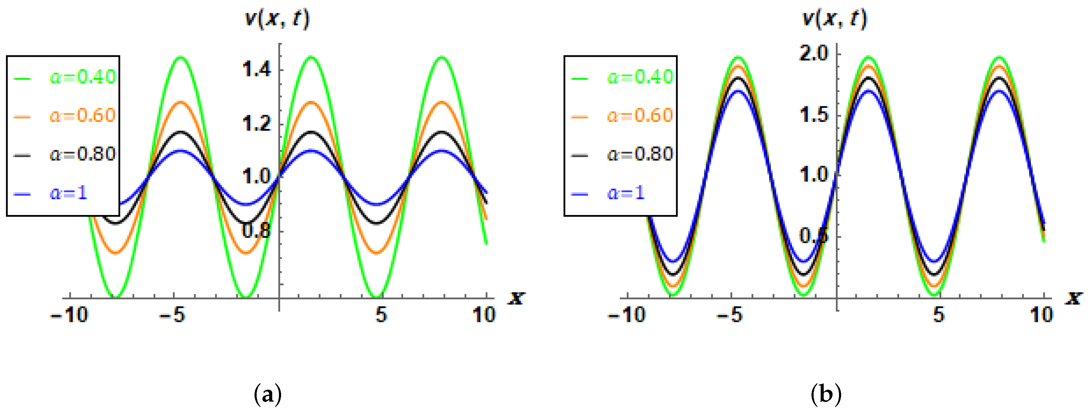
Figure 2 shows the 2D graphs of the exact solution to Equations (34) and (35) at α = 0.4 , 0.6 , 0.8 , 1 , and t = 0.1 , 0.7 . It is clear that with increasing time, the amplitude of the wave increases and the variation in amplitude decreases with different α values.
Application 3.
Consider time-fractional Fitzhugh–Nagumo equation
D t α ν ( x , t ) = D x 2 ν ( x , t ) + ν ( x , t ) ( 1 ν ( x , t ) ) ( ν ( x , t ) θ ) , t > 0 , 0 < α 1 , x R , 0 < θ < 1 ,
subject to the initial condition
ν ( x , 0 ) = 1 1 + e x 2 .
In the special case when α = 1 , the exact solution for Equations (46) and (47) is [19]:
ν ( x , t ) = 1 1 + e x 2 1 2 θ t
Applying LT on both sides of Equations (46) and (47) gives:
V ( x , s ) = 1 s ( 1 + e x 2 ) + D x 2 V ( x , s ) s α + 1 s α L [ ( L 1 [ V ( x , s ) ] ) 2 ] 1 s α L [ ( L 1 [ V ( x , s ) ] ) 3 ] θ s α V ( x , s ) + θ s α L [ ( L 1 [ V ( x , s ) ] ) 2 ] ,
thus, the kth-truncated series of Equation (49) is:
V k ( x , s ) = 1 s ( 1 + e x 2 ) + n = 1 k f n ( x ) s n α + 1 ,
and the kth-LRF, L R e s k ( x , s ) , is:
L R e s k ( x , s ) = V k ( x , s ) 1 s ( 1 + e x 2 ) D x 2 V k ( x , s ) s α 1 s α L [ ( L 1 [ V k ( x , s ) ] ) 2 ] + 1 s α L [ ( L 1 [ V k ( x , s ) ] ) 3 ] + θ s α V k ( x , s ) θ s α L [ ( L 1 [ V k ( x , s ) ] ) 2 ] .
To determine the forms of unknown coefficients f n ( x ) , n = 1 , 2 , , we substitute the kth-truncated series of Equation (50) into the kth-LRF of Equation (51), multiply the new equation by s k α + 1 , and recursively solve the fact lim s s k α + 1 L R e s k ( x , s ) = 0 , k = 1 , 2 , for f k ( x ) . The following are the first few forms of the coefficients f k ( x , s ) :
f 1 ( x ) = e x 2 ( 1 + 2 θ ) 2 1 + e x 2 2 , f 2 ( x ) = e x 2 1 + e x 2 ( 1 + 2 θ ) 2 4 1 + e x 2 3 , f 3 ( x ) = 1 8 ( 1 + e x 2 ) 5 π Γ ( 1 + α ) ( e x 2 ( 1 2 θ ) 2 ( 2 1 + 2 α e x 2 1 + e x 2 ( 2 + θ ) + θ Γ 1 2 + α ( 1 + e x 2 ) π 1 6 e x 2 2 θ + e 2 x ( 1 + 2 θ ) Γ ( 1 + α ) ) ) .
We can express the L-RPS solution of Equation (49) in an infinite series as:
V ( x , s ) = 1 s ( 1 + e x 2 ) e x 2 ( 1 + 2 θ ) 2 s α + 1 ( 1 + e x 2 ) 2 e x 2 ( 1 + e x 2 ) ( 1 + 2 θ ) 2 4 s 2 α + 1 ( 1 + e x 2 ) 3 +
Consequently, the solution of time-fractional Fitzhugh–Nagumo Equations (46) and (47) by taking the inverse LT of Equation (53) is
ν ( x , t ) = 1 ( 1 + e x 2 ) e x 2 ( 1 + 2 θ ) t α 2 Γ ( α + 1 ) ( 1 + e x 2 ) 2 e x 2 ( 1 + e x 2 ) ( 1 + 2 θ ) 2 t 2 α 4 Γ ( 2 α + 1 ) ( 1 + e x 2 ) 3 +
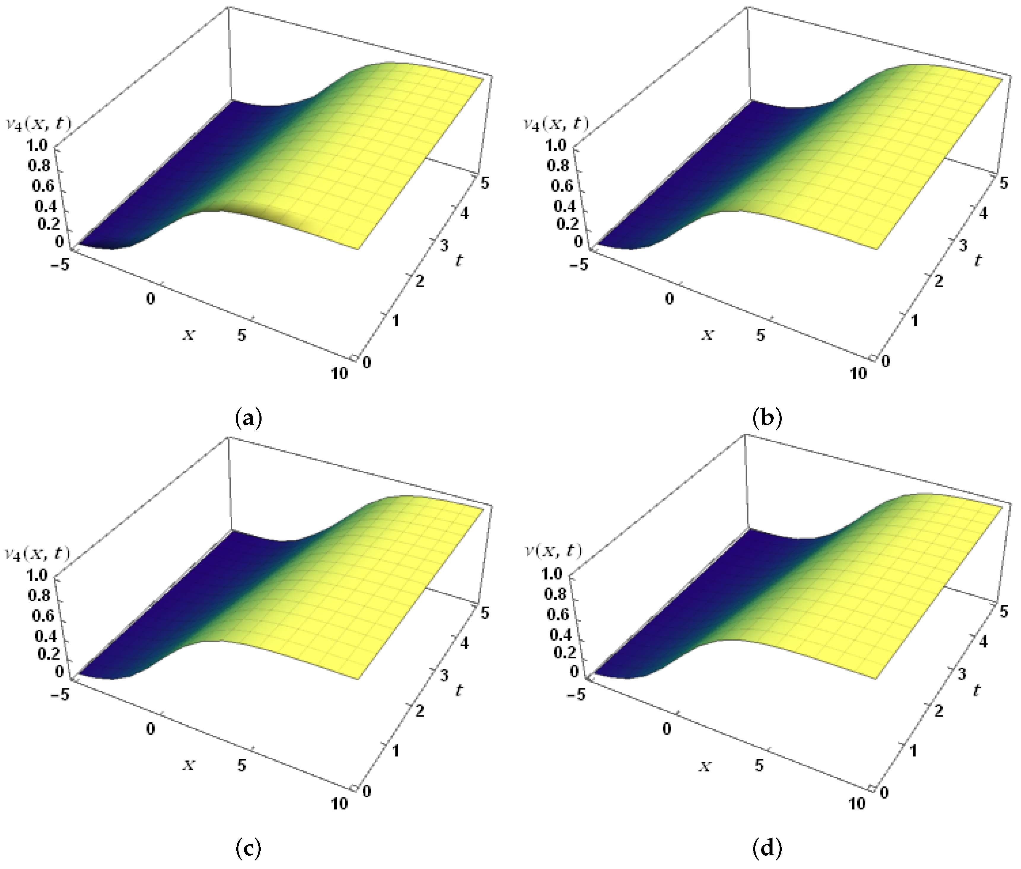
Figure 3 shows the surface graphs of the 4th approximate L-RPS and the exact solutions for Equations (46) and (47) when θ = 0.8 at different values of α . From these sub-figures, it is clear that ν 4 ( x , t ) close the exact solution as the value of α increases.
Application 4.
Consider the generalized Fisher’s equation such that [19]
D t α ν ( x , t ) = D x 2 ν ( x , t ) + ν ( x , t ) ( 1 ν ( x , t ) 6 ) , 0 < α 1 , x > 0 ,
subject to the initial condition
ν ( x , 0 ) = 1 1 + e 3 2 x 3 .
The exact solution for Equations (55) and (56) when α = 1 is ν ( x , t ) = { 1 2 tanh [ 3 4 ( x 5 2 t ) ] + 1 2 } 1 3 .
Taking the LT to both sides of Equation (55), we obtain:
V ( x , s ) = 1 s 1 + e 3 2 x 3 + D x 2 V ( x , s ) s α + V ( x , s ) s α 1 s α L [ ( L 1 [ V ( x , s ) ] ) 7 ] .
Suppose that the k-truncated series solution of Equation (57) takes the following expansion form:
V k ( x , s ) = 1 s 1 + e 3 2 x 3 + n = 1 k f n ( x ) s n α + 1 ,
and the kth-LRF, L R e s k is:
L R e s k ( x , s ) = V k ( x , s ) 1 s 1 + e 3 2 x 3 D x 2 V k ( x , s ) s α V k ( x , s ) s α + 1 s α L [ ( L 1 [ V k ( x , s ) ] ) 7 ] .
By applying L-RPSM, we obtain the first four unknown coefficients f n ( x ) , n = 1 , 2 , 3 in Equation (58), which are as follows:
f 1 ( x ) = 5 e 3 2 x 4 ( 1 + e 3 2 x ) 4 3 , f 2 ( x ) = 25 e 3 2 x ( 3 + e 3 2 x ) 16 ( 1 + e 3 2 x ) 7 3 , f 3 ( x ) = 25 45 e 3 2 x + 123 e 3 x 85 e 9 2 x + 5 e 6 x 21 ( 4 ) α + 1 e 3 x Γ ( 1 2 + α ) π Γ ( 1 + α ) 64 ( 1 + e 3 2 x ) 13 3 .
We can express the solution of Equation (57) obtained by L-RPSM as follows:
V ( x , s ) = 5 e 3 2 x 4 s ( 1 + e 3 2 x ) 4 3 + 25 e 3 2 x ( 3 + e 3 2 x ) 16 s α + 1 ( 1 + e 3 2 x ) 7 3 + .
Therefore, the solution to the generalized Fisher’s equation as in Equations (55) and (56) is:
ν ( x , t ) = 5 e 3 2 x 4 ( 1 + e 3 2 x ) 4 3 + 25 t α e 3 2 x ( 3 + e 3 2 x ) 16 Γ ( α + 1 ) ( 1 + e 3 2 x ) 7 3 + .
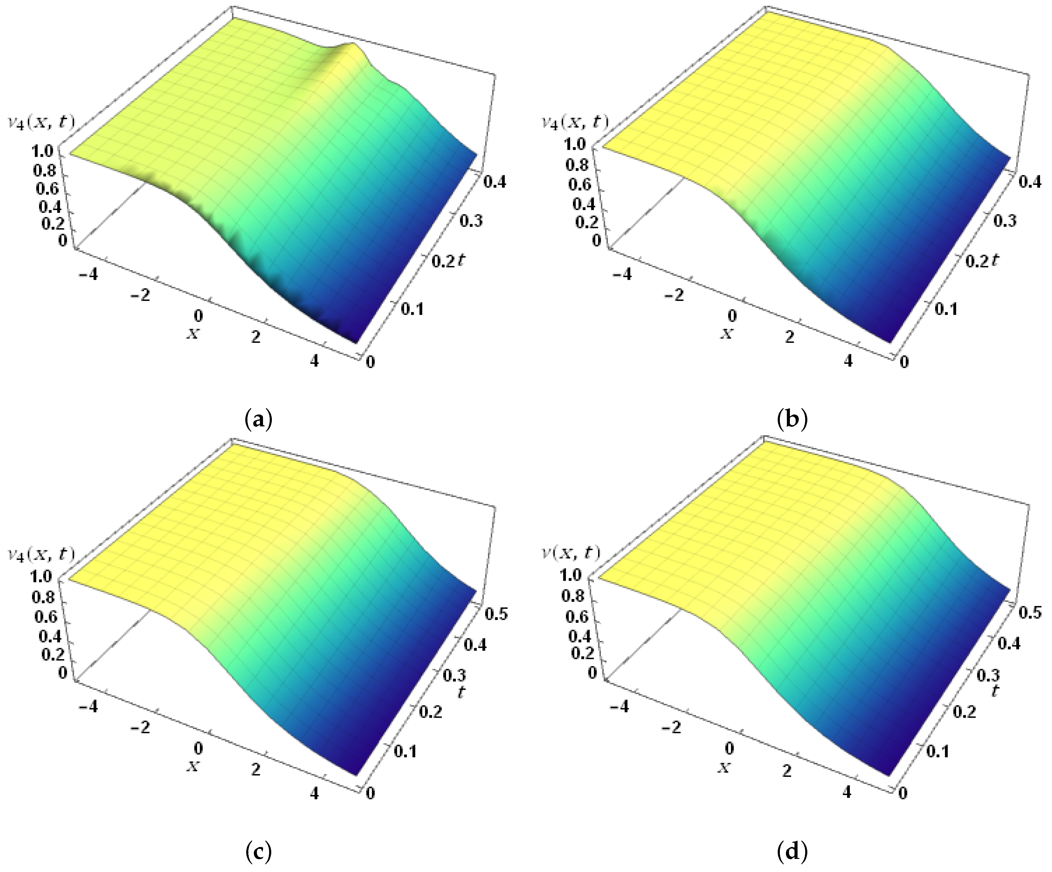
Figure 4 shows the surface graphs of the 4th-AS at different values of α and the exact solutions at α = 1 for Equations (55) and (56). From this figure, it can be seen that the region of convergence of the series solution is small in direction of the t-axis and that the solution becomes smoother with increasing the value of α .
Application 5.
Consider the fractional heat-like equation [14,15,17,18]
D t α ν ( x , t ) = 1 2 x 2 D x 2 ν ( x , t ) , 0 < x 1 , 0 < t 1 , 0 < α < 1 ,
subject to the boundary conditions
ν ( 0 , t ) = 0 , ν ( 1 , t ) = E α ( t α ) ,
with the following initial condition:
ν ( x , 0 ) = x 2 .
By employing the LT to both sides of Equation (63), we obtain:
V ( x , s ) = x 2 s + 1 2 s α x 2 D x 2 V ( x , s ) .
Suppose that the kth-truncated series solution of Equation (66) takes the following expansion form:
V k ( x , s ) = x 2 s + n = 1 k f n ( x ) s n α + 1 ,
and the kth-LRF, L R e s k is:
L R e s k ( x , s ) = V k ( x , s ) x 2 s 1 2 s α x 2 D x 2 V ( x , s ) .
By applying L-RPSM, we obtain the unknown coefficients f n ( x ) , in Equation (67), which are as follows:
f 1 ( x ) = x 2 , f 2 ( x ) = x 2 , f 3 ( x ) = x 2 , f 4 ( x ) = x 2 f n ( x ) = x 2 , n = 5 , 6 , 7 , 8 , .
We can express the L-RPS solution of Equation (66) as follows:
V ( x , s ) = n = 0 x 2 s n α + 1 .
Upon using inverse LT for both sides of Equation (70), the solution of the fractional heat-like equation as in Equations (63)–(65) is
ν ( x , t ) = x 2 n = 0 t n α Γ ( n α + 1 ) = x 2 E α ( t α ) ,
where E α ( z ) is the Mittag–Leffler function and defined as E α ( z ) = n = 0 z n Γ ( 1 + n α ) . It is clear that when α = 1 , we have E 1 ( t ) = e t . Hence, x 2 e t is the exact solution of the classical heat-like equation [14,15,17,18].
Table 1 shows the values of numerical solutions and consecutive errors ( C o n . E r r ) of 17th-AS obtained by L-RPSM for different values of α , where the Con.Err of ν 17 ( x , t ) is C o n . E r r ( x , t ) = | ν 17 ( x , t ) ν 15 ( x , t ) | . From the results, we conclude that L-RPSM provides accurate AS and demonstrates rapid convergence in AS. Moreover, the time taken by the computer to calculate the symbolic and numerical quantities was very limited compared with other methods. That is why we can say that L-RPSM is a simplified and attractive method to find exact and ASs.
Table 2 presents the comparison of absolute error obtained by L-RPSM with the variational iteration method (VIM) [18], the Adomian decomposition method (ADM) [17], the Sinc–Legendre spectral collocation method (S-LCM) [15], and the Jacopi Tau method (JTM) [14] at α = 1 . From Table 2, it is clear that the absolute errors of the AS obtained by L-RPSM of the heat-like equation are small, and we can see that the number of absolute errors decreases as the number of iterations increases.

5. Conclusions

The main objective of this manuscript is to find exact and accurate ASs for the TFRDEs. We noticed during our research that the L-RPSM could be applied under the same conditions that must be met in the RPSM. It requires that the solution has a fractional expansion as in Equation (8). Without this condition, the L-RPSM cannot be used. However, the mechanism of the technique can be applied or adapted for applicability if a suitable expansion is available to the solution of the differential equation. The L-RPSM is generally simple in manual calculations and also fast in the case of using mathematical programs as it depends mainly on calculating the limit at infinity, unlike other methods that need to calculate the fractional derivative in all stages of the solution, resulting in a high cost in terms of effort and speed. So far, the presented technique has been used on limited classes of ordinary and partial differential equations of fractional order. Therefore, the field is open for researchers to adapt the method to apply it to other forms and types of equations, for example, integral equations, integrodifferential equations, and algebraic equations.

Author Contributions

Conceptualization, M.N.O. and T.E.; methodology, T.E.; formal analysis, A.E.-A.; investigation, O.O.; resources, S.E.A.; writing—original draft preparation, S.A.-O.; writing—review and editing, A.E.-A.; writing—review and editing, S.E.A.; supervision, S.A.-O.; project administration, O.O.; and funding acquisition, S.A.-O. All authors have read and agreed to the published version of the manuscript.

Funding

This research received no external funding.

Institutional Review Board Statement

Not applicable.

Informed Consent Statement

Not applicable.

Data Availability Statement

Not applicable.

Acknowledgments

This research was funded by the Deanship for Research and Innovation, Ministry of Education in Saudi Arabia, grant number IFP22UQU4282396DSR051.

Conflicts of Interest

The authors declare that they have no competing interests.

References

  1. Oldham, K.; Spanier, J. The Fractional Calculus Theory and Applications of Differentiation and Integration to Arbitrary Order; Elsevier: Amsterdam, The Netherlands, 1974. [Google Scholar]
  2. Miller, K.; Ross, B. An Introduction to the Fractional Calculus and Fractional Differential Equations; Wiley: Hoboken, NJ, USA, 1993. [Google Scholar]
  3. Podlubny, I. Fractional Differential Equations: An Introduction to Fractional Derivatives, Fractional Differential Equations, to Methods of Their Solution and Some of Their Applications; Elsevier: Amsterdam, The Netherlands, 1998. [Google Scholar]
  4. Mainardi, F. Fractional Calculus and Waves in Linear Viscoelasticity: An Introduction to Mathematical Models; World Scientific: Singapore, 2010. [Google Scholar]
  5. Almeida, R.; Tavares, D.; Torres, D. The Variable-Order Fractional Calculus of Variations; Springer: Berlin/Heidelberg, Germany, 2019. [Google Scholar]
  6. Kilbas, A.; Srivastava, H.; Trujillo, J. Theory and Applications of Fractional Differential Equations; Elsevier: Amsterdam, The Netherlands, 2019. [Google Scholar]
  7. Baleanu, D.; Diethelm, K.; Scalas, E.; Trujillo, J. Fractional Calculus: Models and Numerical Methods; World Scientific: Singapore, 2012. [Google Scholar]
  8. Duan, J.-S.; Rach, R.; Baleanu, D.; Wazwaz, A.-M. A review of the Adomian decomposition method and its applications to fractional differential equations. Commun. Fract. Calc. 2012, 3, 73–99. [Google Scholar]
  9. Magin, R.; Feng, X.; Baleanu, D. Solving the fractional order Bloch equation. Concepts Magn. Reson. Part A Educ. J. 2009, 34, 16–23. [Google Scholar] [CrossRef]
  10. Baleanu, D. New applications of fractional variational principles. Rep. Math. Phys. 2008, 61, 199–206. [Google Scholar] [CrossRef]
  11. Magin, R.; Abdullah, O.; Baleanu, D.; Zhou, X. Anomalous diffusion expressed through fractional order differential operators in the Bloch–Torrey equation. J. Magn. Reson. 2008, 190, 255–270. [Google Scholar] [CrossRef] [PubMed]
  12. Ray, S.; Bera, R. Analytical solution of the Bagley Torvik equation by Adomian decomposition method. Appl. Math. Comput. 2005, 168, 398–410. [Google Scholar] [CrossRef]
  13. Sabatier, J.; Agrawal, O.; Machado, J. Advances in Fractional Calculus; Springer: Berlin/Heidelberg, Germany, 2007. [Google Scholar]
  14. Bhrawy, A.; Zaky, M. A fractional-order Jacobi Tau method for a class of time-fractional PDEs with variable coefficients. Math. Meth. Appl. Sci. 2016, 39, 1765–1779. [Google Scholar] [CrossRef]
  15. Saadatmandi, A.; Dehghan, M.; Azizi, M.-R. The Sinc–Legendre collocation method for a class of fractional convection–diffusion equations with variable coefficients. Commun. Nonlinear Sci. Numer. Simul. 2012, 17, 4125–4136. [Google Scholar] [CrossRef]
  16. Hafez, R.; Zaky, M.; Hendy, A. A novel spectral Galerkin/Petrov–Galerkin algorithm for the multi- dimensional space–time-fractional advection– diffusion–reaction equations with nonsmooth solutions. Math. Comput. Simul. 2021, 190, 678–690. [Google Scholar] [CrossRef]
  17. Momani, S. Analytical approximate solution for fractional heat-like and wave-like equations with variable coefficients using the decomposition method. Appl. Math. Comput. 2005, 165, 459–472. [Google Scholar] [CrossRef]
  18. Molliq, Y.; Noorani, M.; Hashim, I. Variational iteration method for fractional heat-and wave-like equations. Nonlinear Anal. Real World Appl. 2009, 10, 1854–1869. [Google Scholar] [CrossRef]
  19. Loyinmi, A.; Akinfe, T. Exact solutions to the family of Fisher’s reaction–diffusion equation using Elzaki homotopy transformation perturbation method. Eng. Rep. 2020, 2, 12084. [Google Scholar] [CrossRef] [Green Version]
  20. El-Ajou, A.; Oqielat, M.; Al-Zhour, Z.; Momani, S. A class of linear non-homogenous higher order matrix fractional differential equations: Analytical solutions and new technique. Fract. Calc. Appl. Anal. 2020, 23, 356–377. [Google Scholar] [CrossRef]
  21. Eriqat, T.; El-Ajou, A.; Oqielat, M.; Al-Zhour, Z.; Momani, S. A new attractive analytic approach for solutions of linear and nonlinear neutral fractional pantograph equations. Chaos Solit. Fractals 2020, 138, 109957. [Google Scholar] [CrossRef]
  22. El-Ajou, A. Adapting the Laplace transform to create solitary solutions for the nonlinear time-fractional dispersive PDEs via a new approach. Eur. Phys. J. Plus 2021, 136, 229. [Google Scholar] [CrossRef]
  23. Oqielat, M.; Eriqat, T.; Al-Zhour, Z.; Ogilat, O.; El-Ajou, A.; Hashim, I. Construction of fractional series solutions to nonlinear fractional reaction–diffusion for bacteria growth model via Laplace residual power series method. Int. J. Dyn. Control 2022, 1–8. [Google Scholar] [CrossRef]
  24. Eriqat, T.; Oqielat, M.; Al-Zhour, Z.; El-Ajou, A.; Bataineh, A. Revisited Fisher’s equation and logistic system model: A new fractional approach and some modifications. Int. J. Dyn. Control 2022, 1–10. [Google Scholar] [CrossRef]
  25. Oqielat, M.; Eriqat, T.; Ogilat, O.; Odibat, Z.; Al-Zhour, Z.; Hashim, I. Approximate solutions of fuzzy fractional population dynamics model. Eur. Phys. J. Plus 2022, 137, 1–16. [Google Scholar] [CrossRef]
  26. Oqielat, M.; El-Ajou, A.; Al-Zhour, Z.; Eriqat, T.; Al-Smadi, M. A new approach to solving Fuzzy quadratic Riccati differential equations. Int. J. Fuzzy Log. Intell. Syst. 2022, 22, 23–47. [Google Scholar] [CrossRef]
  27. Saadeh, R.; Burqan, A.; El-Ajou, A. Reliable solutions to fractional Lane-Emden equations via Laplace transform and residual error function. Alex. Eng. J. 2022, 61, 10551–10562. [Google Scholar] [CrossRef]
  28. Eriqat, T.; Oqielat, M.; Al-Zhour, Z.; Khammash, G.; El-Ajou, A.; Alrabaiah, H. Exact and numerical solutions of higher-order fractional partial differential equations: A new analytical method and some applications. Pramana J. Phys. 2022, 96, 1–17. [Google Scholar] [CrossRef]
  29. Wazwaz, A.-M.; Gorguis, A. An analytic study of Fisher’s equation by using Adomian decomposition method. Appl. Math. Comput. 2004, 154, 609–620. [Google Scholar] [CrossRef]
  30. Khan, N.; Khan, N.-U.; Ara, A.; Jamil, M. Approximate analytical solutions of fractional reaction–diffusion equations. J. King Saud Univ. Sci. 2012, 24, 111–118. [Google Scholar] [CrossRef] [Green Version]
  31. Tchier, F.; Inc, M.; Korpinar, Z.; Baleanu, D. Solutions of the time-fractional reaction–diffusion equations with residual power series method. Adv. Mech. Eng. 2016, 8, 177. [Google Scholar] [CrossRef] [Green Version]
  32. Alqhtani, M.; Owolabi, K.; Saad, K.; Pindza, E. Efficient numerical techniques for computing the Riesz fractional-order reaction–diffusion models arising in biology. Chaos Solit. Fractals 2022, 161, 112394. [Google Scholar] [CrossRef]
  33. Coronel-Escamilla, A.; Gómez-Aguilar, J.; Torres, L.; Escobar-Jiménez, R.F. A numerical solution for a variable-order reaction–diffusion model by using fractional derivatives with non-local and non-singular kernel. Phys. A 2018, 491, 406–424. [Google Scholar] [CrossRef]
  34. Owolabi, K. Numerical simulation of fractional-order reaction–diffusion equations with the Riesz and Caputo derivatives. Neural Comput. Appl. 2020, 32, 4093–4104. [Google Scholar] [CrossRef]
  35. Matoog, R.T.; Salas, A.H.; Alharbey, R.A.; El-Tantawy, S.A. Rational solutions to the cylindrical nonlinear Schrödinger equation: Rogue waves, breathers, and Jacobi breathers solutions. J. Ocean. Eng. Sci. 2022, 13, 19. [Google Scholar] [CrossRef]
  36. Hou, E.; Hussain, A.; Rehman, A.; Baleanu, D.; Nadeem, S.; Matoog, R.T.; Khan, I.; Sherif, E.S.M. Entropy generation and induced magnetic field in pseudoplastic nanofluid flow near a stagnant point. Sci. Rep. 2021, 11, 23736. [Google Scholar] [CrossRef]
  37. Trikha, P.; Mahmoud, E.E.; Jahanzaib, L.S.; Matoog, R.T.; Abdel-Aty, M. Fractional order biological snap oscillator: Analysis and control. Chaos Solitons Fractals 2021, 145, 110763. [Google Scholar] [CrossRef]
  38. Mahmoud, E.E.; Trikha, P.; Jahanzaib, L.S.; Matoog, R.T. Chaos control and Penta-compound combination anti-synchronization on a novel fractional chaotic system with analysis and application. Results Phys. 2021, 24, 104130. [Google Scholar] [CrossRef]
  39. Alyousef, H.A.; Salas, A.H.; Matoog, R.T.; El-Tantawy, S.A. On the analytical and numerical approximations to the forced damped Gardner Kawahara equation and modeling the nonlinear structures in a collisional plasma. Phys. Fluids 2022, 34, 103105. [Google Scholar] [CrossRef]
  40. Hanna, J.; Rowland, J. Fourier Series, Transforms, and Boundary Value Problems; John Wiley and Sons: Hoboken, NJ, USA, 1990. [Google Scholar]
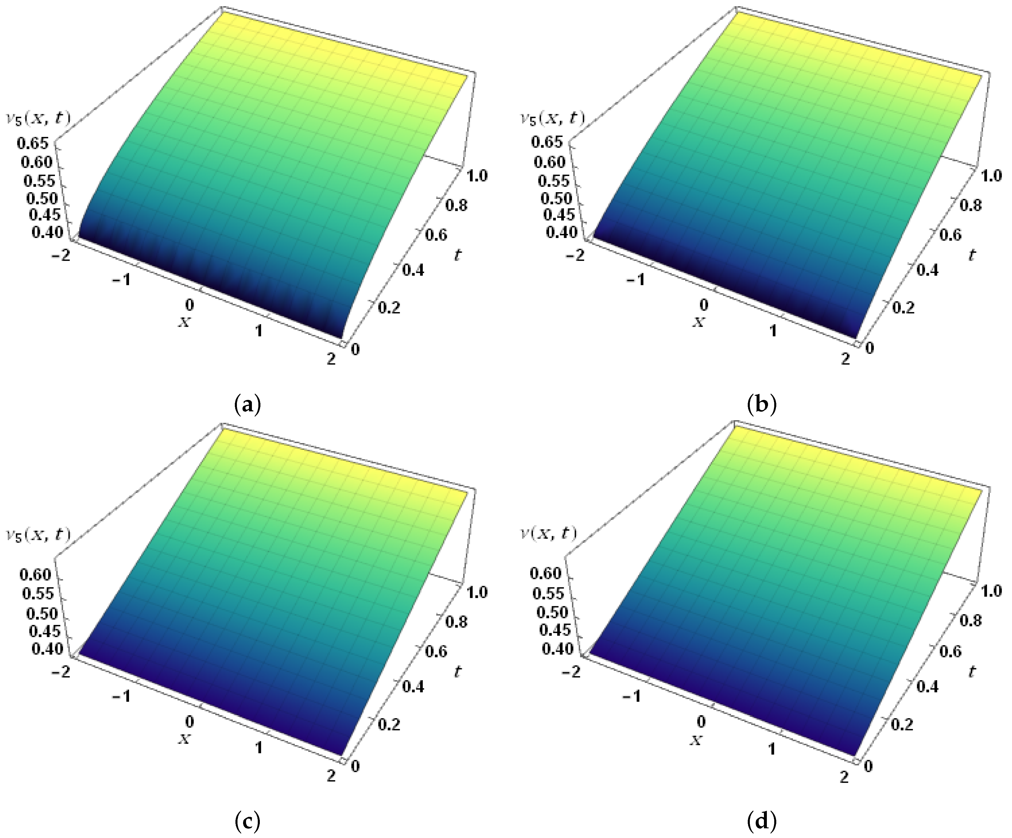
Figure 1. The surface graphs of the exact and ASs of Equations (17) and (18): (a) ν 5 ( x , t ) when α = 0.6 , (b) ν 5 ( x , t ) when α = 0.8 , (c) ν 5 ( x , t ) when α = 1 , and (d) exact solution when α = 1 .
Fractalfract 07 00309 g001
Figure 2. The 2D graphs of the exact solution, ν ( x , t ) , for Equations (34) and (35) at α = 0.4 , 0.6 , 0.8 , 1 : (a) ν 1 ( x , t ) when t = 0.1 , (b) ν 1 ( x , t ) when t = 0.7 .
Fractalfract 07 00309 g002
Figure 3. The surface graphs of the exact and 4th ASs for Equations (46) and (47): (a) ν 4 ( x , t ) when α = 0.6 , (b) ν 4 ( x , t ) when α = 0.8 , (c) ν 4 ( x , t ) when α = 1 , and (d) exact solution ( α = 1 ).
Fractalfract 07 00309 g003
Figure 4. The surface graphs of the exact and ASs for Equations (55) and (56): (a) ν 4 ( x , t ) when α = 0.6 , (b) ν 4 ( x , t ) when α = 0.8 , (c) ν 4 ( x , t ) when α = 1 , and (d) exact solution ( α = 1 ).
Fractalfract 07 00309 g004
Table 1. The numerical solutions and C o n . E r r obtained by the L-RPSM for Application 5 at α = 0.75, 0.9, and 1.
α = 0.75 α = 0.90 α = 1.00
txk = 17Con.Errk = 17Con.Errk = 17Con.Err
0.250.3 0.13491 1.1782 × 10 17 0.12186 7.7226 × 10 22 0.11556 1.0163 × 10 24
0.6 0.53965 4.7127 × 10 17 0.48744 3.0890 × 10 21 0.46225 4.0650 × 10 24
0.9 1.21422 1.0603 × 10 16 1.09675 6.9503 × 10 21 1.04006 9.1463 × 10 24
0.500.3 0.18196 4.9884 × 10 14 0.15953 1.7042 × 10 17 0.14839 6.7567 × 10 20
0.6 0.72782 1.9954 × 10 13 0.63810 6.8169 × 10 17 0.59354 2.7027 × 10 19
0.9 1.63759 4.4896 × 10 13 1.43573 1.5338 × 10 16 1.33546 6.0810 × 10 19
0.750.3 0.24016 6.6573 × 10 12 0.20709 5.9642 × 10 15 0.19053 4.5015 × 10 17
0.6 0.96062 2.6629 × 10 11 0.82837 2.3857 × 10 14 0.76212 1.8006 × 10 16
0.9 2.16140 5.9916 × 10 11 1.86383 5.3677 × 10 14 1.71477 4.0513 × 10 16
1.000.3 0.31373 2.1553 × 10 10 0.26775 3.8243 × 10 13 0.24465 4.5546 × 10 15
0.6 1.25491 8.6213 × 10 10 1.07098 1.5297 × 10 12 0.97858 1.8218 × 10 14
0.9 2.82355 1.9398 × 10 09 2.40970 3.4419 × 10 12 2.20181 4.0991 × 10 14
Table 2. The absolute error of the L-RPS solution obtained for Application 5 compared with various methods at α = 1 .
VIM [18] andS-LCM [15]JTM [14]L-RPSM
txADM [17] N = 15 N = 25 N = 10 N = 15 k = 15 k = 17
0.250.3 1.54 × 10 5 1.09 × 10 6 9.92 × 10 8 2.26 × 10 16 1.05 × 10 16 1.12 × 10 17 1.12 × 10 17
0.6 6.16 × 10 5 2.96 × 10 5 2.70 × 10 6 4.20 × 10 16 3.09 × 10 17 4.49 × 10 17 4.49 × 10 17
0.9 1.38 × 10 4 9.94 × 10 5 1.02 × 10 5 1.51 × 10 15 3.54 × 10 16 1.37 × 10 16 1.37 × 10 16
0.500.3 2.60 × 10 4 6.45 × 10 6 5.56 × 10 7 4.08 × 10 16 1.02 × 10 16 1.64 × 10 17 1.64 × 10 17
0.6 1.03 × 10 3 5.24 × 10 5 4.87 × 10 6 2.47 × 10 16 1.17 × 10 16 6.57 × 10 17 6.56 × 10 17
0.9 2.34 × 10 3 1.47 × 10 4 1.30 × 10 5 2.66 × 10 16 2.45 × 10 16 6.65 × 10 17 6.59 × 10 17
0.750.3 1.39 × 10 3 1.40 × 10 5 1.14 × 10 6 6.24 × 10 16 4.70 × 10 17 3.60 × 10 17 9.16 × 10 18
0.6 5.56 × 10 3 7.67 × 10 5 6.90 × 10 6 9.62 × 10 16 1.74 × 10 16 1.44 × 10 16 3.67 × 10 17
0.9 1.25 × 10 2 2.01 × 10 4 1.59 × 10 5 1.61 × 10 15 1.43 × 10 17 4.82 × 10 16 7.67 × 10 17
1.000.3 4.64 × 10 3 1.83 × 10 5 9.83 × 10 7 1.77 × 10 14 3.11 × 10 16 4.56 × 10 15 7.71 × 10 18
0.6 1.85 × 10 2 9.40 × 10 5 6.40 × 10 6 7.23 × 10 14 2.25 × 10 16 1.83 × 10 14 3.08 × 10 17
0.9 4.18 × 10 2 4.26 × 10 4 2.58 × 10 5 1.62 × 10 13 1.80 × 10 16 4.08 × 10 14 1.86 × 10 16
Disclaimer/Publisher’s Note: The statements, opinions and data contained in all publications are solely those of the individual author(s) and contributor(s) and not of MDPI and/or the editor(s). MDPI and/or the editor(s) disclaim responsibility for any injury to people or property resulting from any ideas, methods, instructions or products referred to in the content.