Investigation of Fractional Order Dynamics of Tuberculosis under Caputo Operator

Abstract

In this article, a new deterministic disease system is constructed to study the influence of treatment adherence as well as awareness on the spread of tuberculosis (TB). The suggested model is composed of six various classes, whose dynamics are discussed in the sense of the Caputo fractional operator. Firstly the model existence of a solution along with a unique solution is checked to determine whether the system has a solution or not. The stability of a solution is also important, so we use the Ulam–Hyers concept of stability. The approximate solution analysis is checked by the technique of Laplace transformation using the Adomian decomposition concept. Such a solution is in series form which is decomposed into smaller terms and the next term is obtained from the previous one. The numerical simulation is established for the obtained schemes using different fractional orders along with a comparison of classical derivatives. Such an analysis will be helpful for testing more dynamics instead of only one type of integer order discussion.

1. Introduction

Tuberculosis (TB) is an infectious disease transmitted by Mycobacterium tuberculosis. It most commonly affects the lungs and is called pulmonary TB. However, in some cases, it can also affect the kidneys, spinal cord, bones, etc. It is an ancient disease, whose evidence has been found in relics from ancient Egypt, India, and China [1]. TB spreads through the air when an active TB patient spits, coughs, or sneezes. A susceptible individual needs to breathe in fewer TB bacteria to become infected. Latent TB patients do not transmit the TB infection. Furthermore, an individual with immune-compromising diseases such as HIV or diabetes is at high risk of TB infection. The symptoms of TB disease are: coughing that lasts for more than two weeks, chest pain, fever, weight loss, fatigue, and night sweats. Though TB is curable by using drug therapy, inappropriate or incomplete treatment can result in severe, resistant TB. Although the BCG vaccine is available to control TB, its effectiveness is still controversial, with a reported efficacy rate of 50% [2]. In spite of significant work carried out in TB control and treatment, still one-third of the population across the world is latently infected, leaving an active TB population for the future. In 2018, about 10 million new TB cases were reported globally, causing more than 1.4 million deaths annually. Moreover, approximately 1.2 million TB patients died with HIV-negative status and 0.25 million died with HIV-positive status in 2018. Most of the deaths were reported in middle- and low-income countries such as India, Nigeria, Indonesia, Pakistan, the Philippines, and South Africa. Southeast Asia contributed approximately 44% of the incidence of TB worldwide [3,4].

The study of the dynamics of contagious diseases transmission relies heavily on mathematical modelling. The literature has a number of mathematical models that have been applied to the study of infectious diseases [5,6,7,8]. To investigate the propagation of the TB infection in the host population with insufficient treatment and isolation, Zhang and Feng [9] reported a deterministic model. The authors of [10] created a model to assess the TB disease’s spread in the Asia–Pacific region. The scientists also took into account the effectiveness of both temporary and partial vaccinations. To explore the impact of detection and adherence on lowering the disease burden, Al-arydah et al proposed a model of TB therapy in their article [11]. Later, Bhunu et al. [12] developed a TB model to analyse the impact of socioeconomic factors on TB infection while taking into account the heterogeneous mixing pattern. Their findings revealed that TB disease is more prevalent in those living in poverty.

Motivated by the above discussion, we consider a TB transmission model, investigating the significance of controlling the TB infection from paper [13,14] as follows:

$$\begin{array}{c}\hfill \left\{\begin{array}{cc}& \frac{d\mathbb{S}}{dt}=\lambda -(1-p)\alpha \frac{\mathbb{S}\mathbb{I}}{\mathbb{N}}-(1-p)v\alpha \frac{\mathbb{S}\mathbb{T}}{\mathbb{N}}-\zeta \mathbb{S},\hfill \\ & \frac{d\mathbb{E}}{dt}=(1-p)c\alpha \frac{\mathbb{S}\mathbb{I}}{\mathbb{N}}+(1-p)cv\alpha \frac{\mathbb{S}\mathbb{T}}{\mathbb{N}}+(1-q)r\mathbb{T}-(\zeta +\beta +\mathrm{\Psi })\mathbb{E},\hfill \\ & \frac{d\mathbb{I}}{dt}=(1-p)(1-c)\alpha \frac{\mathbb{S}\mathbb{I}}{\mathbb{N}}+(1-p)(1-c)v\alpha \frac{\mathbb{S}\mathbb{T}}{\mathbb{N}}+\beta \mathbb{E}-(\zeta +\Delta +\mathrm{\Phi })\mathbb{I},\hfill \\ & \frac{d\mathbb{T}}{dt}=\mathrm{\Phi }\mathbb{I}-(\zeta +\rho +r)\mathbb{T},\hfill \\ & \frac{d\mathbb{R}}{dt}=qr\mathbb{T}+\mathrm{\Psi }\mathbb{E}-\zeta \mathbb{R}.\hfill \end{array}\right.\end{array}$$

(1)

System (1) is studied subject to the initial conditions ${\mathbb{S}}_0,{\mathbb{E}}_0,{\mathbb{I}}_0,{\mathbb{T}}_0,{\mathbb{R}}_0\ge 0.$ Note that the compartments and the used parameters are given in

Table 1. The parameters of the model (1) and their discerption.

Variables	The Physical Representation
$\mathbb{S}$	The number of susceptible individuals
$\mathbb{E}$	The number of Latent class
$\mathbb{I}$	The number of Undetected Infectious class
$\mathbb{T}$	The number of Detected infectious class
$\mathbb{R}$	The number of Recovered class
$\lambda$	New recruitment rate
$\alpha$	Mutual contact rate
v	Decrease rate in infectiousness relative to treatment stages
p	Awareness ratio of human population
q	Treatment adherence level
$\zeta$	Natural death rate
$\rho$	Death rate for class $\mathbb{T}\left(t\right)$
$\Delta$	Death rate for class $\mathbb{I}\left(t\right)$
$\beta$	Reactivation rate
$\mathrm{\Phi }$	Detection rate for active TB cases
$\mathrm{\Psi }$	Recovery rate from $\mathbb{E}\left(t\right)$
r	Rate of Transferring from $\mathbb{T}\left(t\right)$ to $\mathbb{R}\left(t\right)$ or $\mathbb{E}\left(t\right)$
c	Fraction of new infection progress to latent class

and ${\mathbb{S}}_0,{\mathbb{E}}_0,{\mathbb{I}}_0,{\mathbb{T}}_0,{\mathbb{R}}_0$ are initial conditions for all compartments.

The analysis and generalization of the above system can be carried out in the field of modern calculus. It discusses different systems for representing biological and physical phenomena in more detail. Therefore for the past few decades, it has been a very interesting field from the research point of view and many anonymous scientists work through this aspect of generalization. The generalized analysis of modern calculus has attracted a lot of interest from mathematicians and physicists during the last few years. Due to its numerous applications in the engineering and physical sciences for simulating a variety of phenomena in mathematical physics, bioengineering, and chaos theory [15,16,17,18,19,20,21]. In fractional-order calculus mathematical models, the order of the derivatives and integrals is arbitrary. Fractional calculus has many operators that are used in a wide range of applied sciences domains [22,23,24]. The idea of integer-order differentiation is generalized beyond fractional calculus to fractal type differentiation, where the classical differentiations can be retrieved if the fractal dimension becomes one [25,26,27]. Similar to this, if the model being considered has a fractal derivative, the fractal derivative is equal to $\lambda t^{\lambda -1}$. Fractal-fractional calculus is a new field that has evolved as a result of the combining of fractal and fractional notions. Applying this derivative, one can calculate complex problems with both operators. Meanwhile, if we take the fractional order of the derivative we obtain a fractal system, and by taking the noninteger order as unity, then we have a fractional system. This joint operator approach is useful for real-world problems to evaluate the phenomenon where the fractal and fractional derivatives are incompatible separately. Because of this, these operators provided fresh opportunities for the study of complex issues [28,29,30].

Motivated by the above study, we consider a mathematical model of the transmission of the TB dynamics equation in generalized aspects as follows:

$$\begin{array}{c}\hfill \left\{\begin{array}{cc}& \frac{{}^C{d}^{\gamma }\mathbb{S}}{d{t}^{\gamma }}=\lambda -(1-p)\alpha \frac{\mathbb{S}\mathbb{I}}{\mathbb{N}}-(1-p)v\alpha \frac{\mathbb{S}\mathbb{T}}{\mathbb{N}}-\zeta \mathbb{S},\hfill \\ & \frac{{}^C{d}^{\gamma }\mathbb{E}}{d{t}^{\gamma }}=(1-p)c\alpha \frac{\mathbb{S}\mathbb{I}}{\mathbb{N}}+(1-p)cv\alpha \frac{\mathbb{S}\mathbb{T}}{\mathbb{N}}+(1-q)r\mathbb{T}-(\zeta +\beta +\mathrm{\Psi })\mathbb{E},\hfill \\ & \frac{{}^C{d}^{\gamma }\mathbb{I}}{d{t}^{\gamma }}=(1-p)(1-c)\alpha \frac{\mathbb{S}\mathbb{I}}{\mathbb{N}}+(1-p)(1-c)v\alpha \frac{\mathbb{S}\mathbb{T}}{\mathbb{N}}+\beta \mathbb{E}-(\zeta +\Delta +\mathrm{\Phi })\mathbb{I},\hfill \\ & \frac{{}^C{d}^{\gamma }\mathbb{T}}{d{t}^{\gamma }}=\mathrm{\Phi }\mathbb{I}-(\zeta +\rho +r)\mathbb{T},\hfill \\ & \frac{{}^C{d}^{\gamma }\mathbb{R}}{d{t}^{\gamma }}=qr\mathbb{T}+\mathrm{\Psi }\mathbb{E}-\zeta \mathbb{R}\hfill \\ & .{\mathbb{S}}_0,{\mathbb{E}}_0,{\mathbb{I}}_0,{\mathbb{T}}_0,{\mathbb{R}}_0\ge 0,0<\gamma \le 1.\hfill \end{array}\right.\end{array}$$

(2)

2. Preliminaries

We consider it advantageous to recall some basic definitions from [31,32]

Definition 1.

The Riemann–Liouville fractional integral of order γ, for a function $\ell \in L1\left(\right[0,\infty \left)R\right)$, is defined as

$$\begin{array}{c}\hfill I_t^{\gamma }\ell \left(t\right)=\frac{1}{\mathrm{\Gamma }\left(\gamma \right)}\int \frac{\ell \left(\eta \right)}{{(t-\eta )}^{1-\gamma }}d\eta ,\gamma >0,\end{array}$$

assuming the integral on the right is existent.

Definition 2.

The fractional derivative of order γ, in the Caputo sense, is defined as

$$\begin{array}{c}\hfill {}^{\mathcal{C}}{\mathcal{D}}_t^{\gamma }\ell \left(t\right)=\frac{1}{\mathrm{\Gamma }(n-\gamma )}\int \frac{\ell \left(\eta \right)}{{(t-\eta )}^{n-\gamma -1}}{\ell }^n\left(\eta \right)d\eta ,\gamma >0,\end{array}$$

where $n=\left[\gamma \right]+1$ and the integral part on the right exist. If $\gamma \in (0,1)$, then we have

$$\begin{array}{c}\hfill {}^{\mathcal{C}}{\mathcal{D}}_t^{\gamma }\ell \left(t\right)=\frac{1}{\mathrm{\Gamma }(1-\gamma )}\int \frac{\ell \left(\eta \right)}{{(t-\eta )}^{\gamma }}\acute{\ell }\left(\eta \right)d\eta .\end{array}$$

Lemma 1.

The following is true in relation to FODEs [31,32]:

$$\begin{array}{c}\hfill I^{\gamma }{[}^{\mathcal{C}}{\mathcal{D}}_t^{\gamma }\mathrm{\Psi }]\left(t\right)=\mathrm{\Psi }\left(t\right)+a_0+a_1+a_2+\dots +a_{n-1}{t}^{n-1}\end{array}$$

Definition 3.

In the sense of Caputo, we define

$$\begin{array}{c}\hfill \mathcal{L}{[}^{\mathcal{C}}{\mathcal{D}}_t^{\gamma }r\left(t\right)]=s^{\gamma }R\left(s\right)-{\Sigma }_{j=o}^{m-1}{s}^{\gamma -j-1}{r}^k\left(0\right),\gamma \in (m-1,m),m\in {\mathbb{Z}}^{+}\end{array}$$

3. Existence and Uniqueness

In this section, we demonstrate the existence and uniqueness of the system (1) with the use of the fixed point theorem as in [20]. The system (1) under consideration can be written as

$$\begin{array}{c}\hfill \begin{array}{cc}\hfill {}^C{\mathcal{D}}_t^{\gamma }\left(\mathbb{S}\left(t\right)\right)& ={\mathcal{H}}_1(t,\mathbb{S},\mathbb{E},\mathbb{I},\mathbb{T},\mathbb{R}),\hfill \\ \hfill {}^C{\mathcal{D}}_t^{\gamma }\left(\mathbb{E}\left(t\right)\right)& ={\mathcal{H}}_2(t,\mathbb{S},\mathbb{E},\mathbb{I},\mathbb{T},\mathbb{R}),\hfill \\ \hfill {}^C{\mathcal{D}}_t^{\gamma }\left(\mathbb{I}\left(t\right)\right)& ={\mathcal{H}}_3(t,\mathbb{S},\mathbb{E},\mathbb{I},\mathbb{T},\mathbb{R}),\hfill \\ \hfill {}^C{\mathcal{D}}_t^{\gamma }\left(\mathbb{T}\left(t\right)\right)& ={\mathcal{H}}_4(t,\mathbb{S},\mathbb{E},\mathbb{I},\mathbb{T},\mathbb{R}),\hfill \\ \hfill {}^C{\mathcal{D}}_t^{\gamma }\left(\mathbb{R}\left(t\right)\right)& ={\mathcal{H}}_5(t,\mathbb{S},\mathbb{E},\mathbb{I},\mathbb{T},\mathbb{R}),\hfill \end{array}\end{array}$$

(3)

where

$$\begin{array}{c}\hfill \begin{array}{cc}\hfill {\mathcal{H}}_1(t,\mathbb{S},\mathbb{E},\mathbb{I},\mathbb{T},\mathbb{R})& =\lambda -(1-p)\alpha \frac{\mathbb{S}\mathbb{I}}{\mathbb{N}}-(1-p)v\alpha \frac{\mathbb{S}\mathbb{T}}{\mathbb{N}}-\zeta \mathbb{S},\hfill \\ \hfill {\mathcal{H}}_2(t,\mathbb{S},\mathbb{E},\mathbb{I},\mathbb{T},\mathbb{R})& =(1-p)c\alpha \frac{\mathbb{S}\mathbb{I}}{\mathbb{N}}+(1-p)cv\alpha \frac{\mathbb{S}\mathbb{T}}{\mathbb{N}}+(1-q)r\mathbb{T}-(\zeta +\beta +\mathrm{\Psi })\mathbb{E},\hfill \\ \hfill {\mathcal{H}}_3(t,\mathbb{S},\mathbb{E},\mathbb{I},\mathbb{T},\mathbb{R})& =(1-p)(1-c)\alpha \frac{\mathbb{S}\mathbb{I}}{\mathbb{N}}+(1-p)(1-c)v\alpha \frac{\mathbb{S}\mathbb{T}}{\mathbb{N}}+\beta \mathbb{E}-(\zeta +\Delta +\mathrm{\Phi })\mathbb{I},\hfill \\ \hfill {\mathcal{H}}_4(t,\mathbb{S},\mathbb{E},\mathbb{I},\mathbb{T},\mathbb{R})& =\mathrm{\Phi }\mathbb{I}-(\zeta +\rho +r)\mathbb{T},\hfill \\ \hfill {\mathcal{H}}_5(t,\mathbb{S},\mathbb{E},\mathbb{I},\mathbb{T},\mathbb{R})& =qr\mathbb{T}+\mathrm{\Psi }\mathbb{E}-\zeta \mathbb{R}.\hfill \end{array}\end{array}$$

(4)

The system (1) is represented as

$$\begin{array}{c}\hfill \left\{\begin{array}{c}{}^C{\mathcal{D}}_t^{\gamma }\left(\mathbb{U}\left(t\right)\right)=\mathbb{Z}(t,\mathbb{U}\left(t\right)),\hfill \\ \mathbb{U}\left(0\right)={\mathbb{U}}_0\ge 0,\hfill \end{array}\right.\end{array}$$

(5)

where

$$\begin{array}{c}\hfill \left\{\begin{array}{c}\mathbb{U}\left(t\right)={(\mathbb{S},\mathbb{E},\mathbb{I},\mathbb{T},\mathbb{R})}^{Tr},\hfill \\ \mathbb{U}\left(0\right)={({\mathbb{S}}_0,{\mathbb{E}}_0,{\mathbb{I}}_0,{\mathbb{T}}_0,{\mathbb{R}}_0)}^{Tr},\hfill \\ \mathbb{Z}(t,\mathbb{U}\left(t\right))=({\mathcal{H}}_i{(t,\mathbb{S},\mathbb{E},\mathbb{I},\mathbb{T},\mathbb{R})}^{Tr},i=1,2,3,4,5,\hfill \end{array}\right.\end{array}$$

(6)

where transpose of the vector is represented by ${(.)}^{Tr}$. Note that the system (5) can be expressed in the form:

$$\begin{array}{c}\hfill \mathbb{U}\left(t\right)={\mathbb{U}}_0+{\mathcal{J}}^{\gamma }\mathbb{Z}(t,\mathbb{U}\left(t\right))={\mathbb{U}}_0+\frac{1}{\mathrm{\Gamma }\left(\gamma \right)}{\int }_0^t{(t-s)}^{\gamma -1}\mathbb{Z}(s,\mathbb{U}\left(s\right))ds.\end{array}$$

(7)

Assume that the continuous function on $\mathbb{Z}$ is the Banach Space established on the interval $[0,b]$ with $\parallel \mathbb{U}\parallel ={max}_{t\in \mathcal{J}}\left|\mathbb{U}\right|$ be $\mathbf{F}=C\left(\right[0,b];\mathbb{Z})$. In the following, we will use the assumption:

${\mathbf{C}}_{\mathbf{1}}$: One can associate the constants, e.g., ${\mathcal{K}}_{\mathbb{Z}}>0,$${\mathcal{M}}_{\mathbb{Z}}>0$ belonging to $\left(C\right[0,b],R)$ in such a fashion that for all $(t,\mathbb{U})\in \mathcal{J}\times R^5$, we have

$$\left|\mathbb{Z}(t,\mathbb{U})\right|\le {\mathcal{K}}_{\mathbb{Z}}+M_{\mathbb{Z}}\left|\mathbb{U}\right|.$$

${\mathbf{C}}_{\mathbf{2}}$: There is a constant ${\mathcal{L}}_{\mathbb{Z}}>0$ in such a way that for every ${\mathbb{U}}_1,{\mathbb{U}}_2\in C\left([\mathcal{J},R]\right),$

$$|\mathbb{Z}(t,{\mathbb{U}}_1\left(t\right))-\mathbb{Z}(t,{\mathbb{U}}_2\left(t\right))|\le {\mathcal{L}}_{\mathbb{Z}}|{\mathbb{U}}_1\left(t\right)-{\mathbb{U}}_2\left(t\right)|.$$

We demonstrate the uniqueness of the solution with the aid of the following theorem [19].

Theorem 1.

With hypotheses $\left({\mathbf{C}}_{\mathbf{2}}\right),\mathbb{Z}\in C\left([\mathcal{J},\mathbf{R}]\right)$ along with the mappings $\mathcal{J}\times {\mathbf{R}}^5$ bounded subset to relatively compact-subset of $\mathbf{R}$. In case $\theta {\mathcal{L}}_{\mathbb{Z}}<1$, Equation (5) possesses a unique solution where $\theta =\frac{T^{\gamma }}{\mathrm{\Gamma }(\gamma +1)}.$

Proof. 

Let us express the operator $\mathbf{F}:\mathbf{X}\to \mathbf{X}$ and consider ${\mathbb{U}}_1{\mathbb{U}}_2\in \mathbf{X}$ then

$$\begin{array}{ccc}\hfill \parallel \mathbf{F}\left({\mathbb{U}}_1\right)-\mathbf{F}\left({\mathbb{U}}_2\right)\parallel & =& \underset{t\in [0,\mathcal{T}]}{max}|\frac{1}{\mathrm{\Gamma }\left(\gamma \right)}{\int }_0^t{(t-s)}^{\gamma -1}\mathbb{Z}(s,{\mathbb{U}}_1\left(s\right))ds\hfill \\ & -& \frac{1}{\mathrm{\Gamma }\left(\gamma \right)}{\int }_0^t{(t-s)}^{\gamma -1}\mathbb{Z}(s,\overline{{\mathbb{U}}_2}\left(s\right))ds|,\hfill \\ & \le & \frac{T^{\gamma }}{\mathrm{\Gamma }(\gamma +1)}{L}_{\mathbb{Z}}\parallel {\mathbb{U}}_1-{\mathbb{U}}_2\parallel \hfill \\ & \le & \theta L_{\mathbb{Z}}\parallel {\mathbb{U}}_1-{\mathbb{U}}_2\parallel .\hfill \end{array}$$

(8)

Consequently, by the principle of Banach contraction, we may deduce that the system (5) possesses a unique solution on $\mathcal{J}.$ □

Next, to demonstrate the existence of the solution of (2), we use the Schauder fixed-point theory.

Lemma 2.

Assume a convex, closed and bounded subset of a Banach space $\mathbf{X}$ be $\mathcal{M}.$ Consider the operator be ${\mathbf{F}}_1,{\mathbf{F}}_2$, then the following:

• ${\mathbf{F}}_1{\mathbb{U}}_1+{\mathbf{F}}_2{\mathbb{U}}_2,$ only if ${\mathbb{U}}_1,{\mathbb{U}}_2\in \mathcal{M};$
• The operator ${\mathbf{F}}_1$ is compact and continuous;
• ${\mathbf{F}}_2$ is a contraction mapping.

There exists $u\in \mathcal{M}$, such that $u={\mathbf{F}}_{1}u+{\mathbf{F}}_{2}u.$

Theorem 2.

Using the assumption $\left({\mathbf{C}}_{\mathbf{1}}\right)$ and $\left({\mathbf{C}}_{\mathbf{2}}\right)$ with $\mathbb{Z}:\mathcal{J}\times {\mathbf{R}}^{\mathbf{5}}\to \mathbf{R}$. The system described in (2) contains at least one solution on $\mathcal{J}$ whenever

$${\mathcal{L}}_{\mathbb{Z}}\parallel {\mathbb{U}}_1\left(t_0\right)-{\mathbb{U}}_2\left(t_0\right)\parallel <1.$$

Proof. 

Assume that ${max}_{t\in \mathcal{J}}\left|\mathcal{K}\left(t\right)\right|=\parallel \mathcal{K}\parallel$ and $\rho \ge \parallel \mathbb{U}0\parallel +\gamma \parallel \mathcal{K}\parallel$, with $\mathbf{B}\rho =\{\mathbb{U}\in \mathbf{E}:\parallel \mathbb{U}\parallel \le \rho \}.$ For each ${\mathbf{F}}_1,{\mathbf{F}}_2$ on $\mathbf{B}\rho$ given as

$$\begin{array}{c}\hfill \left({\mathbf{F}}_1\mathbb{U}\right)\left(t\right)=\frac{1}{\mathrm{\Gamma }\left(\gamma \right)}{\int }_0^t{(t-s)}^{\gamma -1}\mathbb{Z}(s,\mathbb{U}\left(s\right))ds,t\in \mathcal{J},\end{array}$$

and $\left({\mathbf{F}}_2\mathbb{U}\right)\left(t\right)=\mathbb{U}\left(t_0\right)$, $t\in \mathcal{J}.$ So, fr all ${\mathbf{F}}_1,{\mathbf{F}}_2\in \mathbf{B}\rho ,$ we obtain

$$\begin{array}{c}\hfill \begin{array}{cc}\hfill \parallel \left({\mathbf{F}}_1{\mathbb{U}}_1\right)\left(t\right)+\left({\mathbf{F}}_2{\mathbb{U}}_2\right)\left(t\right)\parallel & \le \parallel {\mathbb{U}}_0\parallel +\frac{1}{\mathrm{\Gamma }\left(\gamma \right)}{\int }_0^t{(t-s)}^{\gamma -1}\parallel \mathbb{Z}(s,{\mathbf{F}}_1\left(s\right))\parallel ds,\hfill \\ & \le \parallel {\mathbb{U}}_0\parallel +\gamma \parallel \mathcal{K}\parallel \hfill \\ & \le \rho <\infty .\hfill \end{array}\end{array}$$

(9)

Hence, ${\mathbf{F}}_1{\mathbb{U}}_1+{\mathbf{F}}_2{\mathbb{U}}_2\in \mathbf{B}\rho$.

Now, we prove the contraction of ${\mathbf{F}}_2$.

By hypothesis for any $t\in \mathcal{J}$ and ${\mathbf{F}}_1,{\mathbf{F}}_2\in \mathbf{B}\rho$, one should have

$$\begin{array}{c}\hfill \parallel \left({\mathbf{F}}_1{\mathbb{U}}_1\right)\left(t\right)-\left({\mathbf{F}}_2{\mathbb{U}}_2\right)\left(t\right)\parallel \le \parallel {\mathbf{F}}_1\left(t_0\right)-{\mathbf{F}}_2\left(t_0\right)\parallel .\end{array}$$

(10)

Since we have a continuous function $\mathbb{Z}$, thus ${\mathbf{F}}_1$ is continuous. Further, for every $t\in \mathcal{J}$ and ${\mathbb{U}}_1\in \mathbf{B}\rho$,

$$\parallel {\mathbf{F}}_1\mathbb{U}\parallel \le \parallel \mathcal{K}\parallel <\infty .$$

Consequently, one may deduce the uniform boundedness of ${\mathbf{F}}_1$. Finally, we demonstrate that ${\mathbf{F}}_1$ is compact. For this purpose we assume that

$max(t,\mathbb{U})\in (\mathcal{J}\times {\mathbf{B}}_{\rho })\left|\mathbb{Z}(s,\mathbb{U}\left(s\right))\right|={\mathbb{Z}}^{*}$, which gives

$$\begin{array}{ccc}\hfill |\left({\mathbf{F}}_1\mathbb{U}\right)\left(t_2\right)-\left({\mathbf{F}}_1\mathbb{U}\right)\left(t_1\right)|& =& \frac{1}{\mathrm{\Gamma }\left(\gamma \right)}|{\int }_0^t\left[{(t_2-s)}^{\gamma -1}-{(t_1-s)}^{\gamma -1}\right]\mathbb{Z}(s,\mathbb{U}\left(s\right))ds+{\int }_{t_1}^{t_2}{(t_2-s)}^{\gamma -1}\mathbb{Z}(s,\mathbb{U}\left(s\right))|\hfill \\ & & \le \frac{{\mathbb{Z}}^{*}}{\mathrm{\Gamma }\left(\gamma \right)}\left[2{(t_2-t_1)}^{\gamma }+(t_2^{\gamma }-t_1^{\gamma })\right]\to 0\mathrm{as}{t}_2\to t_1.\hfill \end{array}$$

(11)

The operator $\mathbf{F}1$ is relatively compact $\mathbf{B}\rho$ and hence $\mathbf{F}1$ is completely continuous in light of the well-known “Arzela–Ascoli theorem.” By proving assertions of Lemma 2, we conclude that the suggested system (2) possesses at least one solution. □

4. Approximate Solution by LADM

This section examines the proposed model’s approximative series solutions using the technique of Laplace–Adomian decomposition. The calculation through this technique is achieved by decomposing the whole quantity into small ones and the non-linear terms are computed with an Adomian polynomial. The Laplace transforms on each quantity are then very easy by starting from the initial value-like iteration. The next term is obtained from the previous one. In the following, we examine the general approach for the considered model, (2) subjected to initial conditions as in [21]. Taking Laplace transform of both sides of the system (2) we may write

$$\begin{array}{ccc}\hfill \mathcal{L}\left[{}^C{\mathcal{D}}_t^{\gamma }\mathbb{S}\left(t\right)\right]& =& \mathcal{L}\left[\lambda -(1-p)\alpha \frac{\mathbb{S}\mathbb{I}}{\mathbb{N}}-(1-p)v\alpha \frac{\mathbb{S}\mathbb{T}}{\mathbb{N}}-\zeta \mathbb{S}\right],\hfill \\ \hfill \mathcal{L}\left[{}^C{\mathcal{D}}_t^{\gamma }\mathbb{E}\left(t\right)\right]& =& \mathcal{L}\left[(1-p)c\alpha \frac{\mathbb{S}\mathbb{I}}{\mathbb{N}}+(1-p)cv\alpha \frac{\mathbb{S}\mathbb{T}}{\mathbb{N}}+(1-q)r\mathbb{T}-(\zeta +\beta +\mathrm{\Psi })\mathbb{E}\right],\hfill \\ \hfill \mathcal{L}\left[{}^C{\mathcal{D}}_t^{\gamma }\mathbb{I}\left(t\right)\right]& =& \mathcal{L}\left[(1-p)(1-c)\alpha \frac{\mathbb{S}\mathbb{I}}{\mathbb{N}}+(1-p)(1-c)v\alpha \frac{\mathbb{S}\mathbb{T}}{\mathbb{N}}+\beta \mathbb{E}-(\zeta +\Delta +\mathrm{\Phi })\mathbb{I}\right],\hfill \\ \hfill \mathcal{L}\left[{}^C{\mathcal{D}}_t^{\gamma }\mathbb{T}\left(t\right)\right]& =& \mathcal{L}\left[\mathrm{\Phi }\mathbb{I}-(\zeta +\rho +r)\mathbb{T}\right],\hfill \\ \hfill \mathcal{L}\left[{}^C{\mathcal{D}}_t^{\gamma }\mathbb{R}\left(t\right)\right]& =& \mathcal{L}\left[qr\mathbb{T}+\mathrm{\Psi }\mathbb{E}-\zeta \mathbb{R}\right].\hfill \end{array}$$

(12)

Applying the initial conditions (12), we obtain

$$\begin{array}{ccc}\hfill \mathcal{L}\left[\mathbb{S}\left(t\right)\right]& =& \frac{M_1}{s}+\frac{1}{s^{\gamma }}\mathcal{L}[\lambda -(1-p)\alpha \frac{\mathbb{S}\mathbb{I}}{\mathbb{N}}-(1-p)v\alpha \frac{\mathbb{S}\mathbb{T}}{\mathbb{N}}-\zeta \mathbb{S}],\hfill \\ \hfill \mathcal{L}\left[\mathbb{E}\left(t\right)\right]& =& \frac{M_2}{s}+\frac{1}{s^{\gamma }}\mathcal{L}\left[(1-p)c\alpha \frac{\mathbb{S}\mathbb{I}}{\mathbb{N}}+(1-p)cv\alpha \frac{\mathbb{S}\mathbb{T}}{\mathbb{N}}+(1-q)r\mathbb{T}-(\zeta +\beta +\mathrm{\Psi })\mathbb{E}\right],\hfill \\ \hfill \mathcal{L}\left[\mathbb{I}\left(t\right)\right]& =& \frac{M_3}{s}+\frac{1}{s^{\gamma }}\mathcal{L}\left[(1-p)(1-c)\alpha \frac{\mathbb{S}\mathbb{I}}{\mathbb{N}}+(1-p)(1-c)v\alpha \frac{\mathbb{S}\mathbb{T}}{\mathbb{N}}+\beta \mathbb{E}-(\zeta +\Delta +\mathrm{\Phi })\mathbb{I}\right],\hfill \\ \hfill \mathcal{L}\left[\mathbb{T}\left(t\right)\right]& =& \frac{M_4}{s}+\frac{1}{s^{\gamma }}\mathcal{L}\left[\mathrm{\Phi }\mathbb{I}-(\zeta +\rho +r)\mathbb{T}\right],\hfill \\ \hfill \mathcal{L}\left[\mathbb{R}\left(t\right)\right]& =& \frac{M_5}{s}+\frac{1}{s^{\gamma }}\mathcal{L}\left[qr\mathbb{T}+\mathrm{\Psi }\mathbb{E}-\zeta \mathbb{R}\right].\hfill \end{array}$$

(13)

Next, consider the following series solution of $\mathbb{S},\mathbb{E},\mathbb{I},\mathbb{T},\mathbb{R}$ with infinite terms

$$\begin{array}{c}\hfill \begin{array}{ccccccccccc}\hfill \mathbb{S}\left(t\right)& =\hfill & \sum _{n=0}^{\infty }{\mathbb{S}}_n\left(t\right),\mathbb{E}\left(t\right)& =& \sum _{n=0}^{\infty }{\mathbb{E}}_n\left(t\right),\mathbb{I}\left(t\right)& =& \sum _{n=0}^{\infty }{\mathbb{I}}_n\left(t\right),\mathbb{T}\left(t\right)& =& \sum _{n=0}^{\infty }{\mathbb{T}}_n\left(t\right),\mathbb{R}\left(t\right)& =& \sum _{n=0}^{\infty }{\mathbb{R}}_n\left(t\right)\end{array}\end{array}$$

(14)

where

$$\mathbb{S}\left(t\right)\mathbb{I}\left(t\right)=\sum _{n=0}^{\infty }{p}_n\left(t\right),\mathbb{S}\left(t\right)\mathbb{T}\left(t\right)=\sum _{n=0}^{\infty }{q}_n\left(t\right).$$

Next, we decompose Equation (14) into the Adomian polynomial, where

$$\begin{array}{c}\hfill \begin{array}{ccccc}\hfill p_n\left(t\right)& =\hfill & \frac{1}{n!}\frac{d^n}{d{\lambda }^n}{\left[\sum _{k=0}^n{\lambda }^k\mathbb{S}\left(t\right)\sum _{k=0}^n{\lambda }^k{\mathbb{I}}_k\left(t\right)\right]}_{\lambda =0}{q}_n\left(t\right)& =& \frac{1}{n!}\frac{d^n}{d{\lambda }^n}{\left[\sum _{k=0}^n{\lambda }^k\mathbb{S}\left(t\right)\sum _{k=0}^n{\lambda }^k{\mathbb{T}}_k\left(t\right)\right]}_{\lambda =0}\end{array}\end{array}$$

(15)

Using (14) and (15) in (13) and comparing like terms of each sides, we have

$$\begin{array}{c}\hfill \begin{array}{cc}\hfill & \mathcal{L}\left[{\mathbb{S}}_0\left(t\right)\right]=\frac{{\mathrm{M}}_1}{s},\mathcal{L}\left[{\mathbb{E}}_0\left(\mathrm{t}\right)\right]=\frac{{\mathrm{M}}_2}{s},\mathcal{L}\left[{\mathbb{I}}_0\left(\mathrm{t}\right)\right]=\frac{{\mathrm{M}}_3}{s},\mathcal{L}\left[{\mathbb{T}}_0\left(\mathrm{t}\right)\right]=\frac{{\mathrm{M}}_4}{s},\mathcal{L}\left[{\mathbb{R}}_0\left(\mathrm{t}\right)\right]=\frac{{\mathrm{M}}_5}{s}\hfill \\ & \mathcal{L}\left[{\mathbb{S}}_1\left(\mathrm{t}\right)\right]=\frac{1}{s^{\gamma }}\mathcal{L}\left[\lambda -(1-p)\alpha \frac{p_0}{\mathbb{N}}-(1-p)v\alpha \frac{q_0}{\mathbb{N}}-\zeta {\mathbb{S}}_0)\right],\hfill \\ & \mathcal{L}\left[{\mathbb{E}}_1\left(t\right)\right]=\frac{1}{s^{\gamma }}\mathcal{L}\left[(1-p)c\alpha \frac{p_0}{\mathbb{N}}+(1-p)cv\alpha \frac{q_0}{\mathbb{N}}+(1-q)r{\mathbb{T}}_0-(\zeta +\beta +\mathrm{\Psi }){\mathbb{E}}_0\right],\hfill \\ & \mathcal{L}\left[{\mathbb{I}}_1\left(t\right)\right]=\frac{1}{s^{\gamma }}\mathcal{L}\left[(1-p)(1-c)\alpha \frac{p_0}{\mathbb{N}}+(1-p)(1-c)v\alpha \frac{q_0}{\mathbb{N}}+\beta {\mathbb{E}}_0-(\zeta +\Delta +\mathrm{\Phi }){\mathbb{I}}_0\right],\hfill \\ & \mathcal{L}\left[{\mathbb{T}}_1\left(\mathrm{t}\right)\right]=\frac{1}{s^{\gamma }}\mathcal{L}\left[\mathrm{\Phi }{\mathbb{I}}_0-(\zeta +\rho +r){\mathbb{T}}_0\right],\hfill \\ & \mathcal{L}\left[{\mathbb{R}}_1\left(\mathrm{t}\right)\right]=\frac{1}{s^{\gamma }}\mathcal{L}\left[qr{\mathbb{T}}_0+\mathrm{\Psi }{\mathbb{E}}_0-\zeta {\mathbb{R}}_0\right],\hfill \\ & \mathcal{L}\left[{\mathbb{S}}_2\left(\mathrm{t}\right)\right]=\frac{1}{s^{\gamma }}\mathcal{L}\left[\lambda -(1-p)\alpha \frac{p_1}{\mathbb{N}}-(1-p)v\alpha \frac{q_1}{\mathbb{N}}-\zeta {\mathbb{S}}_1)\right],\hfill \\ & \mathcal{L}\left[{\mathbb{E}}_2\left(t\right)\right]=\frac{1}{s^{\gamma }}\mathcal{L}\left[(1-p)c\alpha \frac{p_1}{\mathbb{N}}+(1-p)cv\alpha \frac{q_1}{\mathbb{N}}+(1-q)r{\mathbb{T}}_1-(\zeta +\beta +\mathrm{\Psi }){\mathbb{E}}_1\right],\hfill \\ & \mathcal{L}\left[{\mathbb{I}}_2\left(t\right)\right]=\frac{1}{s^{\gamma }}\mathcal{L}\left[(1-p)(1-c)\alpha \frac{p_1}{\mathbb{N}}+(1-p)(1-c)v\alpha \frac{q_1}{\mathbb{N}}+\beta {\mathbb{E}}_1-(\zeta +\Delta +\mathrm{\Phi }){\mathbb{I}}_1\right],\hfill \\ & \mathcal{L}\left[{\mathbb{T}}_2\left(\mathrm{t}\right)\right]=\frac{1}{s^{\gamma }}\mathcal{L}\left[\mathrm{\Phi }{\mathbb{I}}_1-(\zeta +\rho +r){\mathbb{T}}_1\right],\hfill \\ & \mathcal{L}\left[{\mathbb{R}}_2\left(\mathrm{t}\right)\right]=\frac{1}{s^{\gamma }}\mathcal{L}\left[qr{\mathbb{T}}_1+\mathrm{\Psi }{\mathbb{E}}_1-\zeta {\mathbb{R}}_1\right],\hfill \\ & ⋮\hfill \\ & \mathcal{L}\left[{\mathbb{S}}_{\mathrm{n}+1}\left(\mathrm{t}\right)\right]=\frac{1}{s^{\gamma }}\mathcal{L}\left[\lambda -(1-p)\alpha \frac{p_n}{\mathbb{N}}-(1-p)v\alpha \frac{q_n}{\mathbb{N}}-\zeta {\mathbb{S}}_n)\right],\hfill \\ & \mathcal{L}\left[{\mathbb{E}}_{n+1}\left(t\right)\right]=\frac{1}{s^{\gamma }}\mathcal{L}\left[(1-p)c\alpha \frac{p_n}{\mathbb{N}}+(1-p)cv\alpha \frac{q_n}{\mathbb{N}}+(1-q)r{\mathbb{T}}_n-(\zeta +\beta +\mathrm{\Psi }){\mathbb{E}}_n\right],\hfill \\ & \mathcal{L}\left[{\mathbb{I}}_{n+1}\left(t\right)\right]=\frac{1}{s^{\gamma }}\mathcal{L}\left[(1-p)(1-c)\alpha \frac{p_n}{\mathbb{N}}+(1-p)(1-c)v\alpha \frac{q_n}{\mathbb{N}}+\beta {\mathbb{E}}_n-(\zeta +\Delta +\mathrm{\Phi }){\mathbb{I}}_n\right],\hfill \\ & \mathcal{L}\left[{\mathbb{T}}_{\mathrm{n}+1}\left(\mathrm{t}\right)\right]=\frac{1}{s^{\gamma }}\mathcal{L}\left[\mathrm{\Phi }{\mathbb{I}}_n-(\zeta +\rho +r){\mathbb{T}}_n\right],\hfill \\ & \mathcal{L}\left[{\mathbb{R}}_{\mathrm{n}+1}\left(\mathrm{t}\right)\right]=\frac{1}{s^{\gamma }}\mathcal{L}\left[qr{\mathbb{T}}_1+\mathrm{\Psi }{\mathbb{E}}_n-\zeta {\mathbb{R}}_n\right].\hfill \end{array}\end{array}$$

(16)

Applying the inverse Laplace transform, we can write from Equation (16):

$$\begin{array}{c}\hfill \begin{array}{cc}\hfill & \left[{\mathbb{S}}_0\left(\mathrm{t}\right)\right]={\mathcal{L}}^{-1}\left[\frac{{\mathrm{M}}_1}{s}\right],{\mathcal{L}}^{-1}\left[{\mathbb{E}}_0\left(\mathrm{t}\right)\right]=\left[\frac{{\mathrm{M}}_2}{s}\right],\left[{\mathbb{I}}_0\left(\mathrm{t}\right)\right]={\mathcal{L}}^{-1}\left[\frac{{\mathrm{M}}_3}{s}\right],\hfill \\ & {\mathcal{L}}^{-1}\left[{\mathbf{T}}_0\left(\mathrm{t}\right)\right]=\left[\frac{{\mathrm{M}}_4}{s}\right],{\mathcal{L}}^{-1}\left[{\mathbf{R}}_0\left(\mathrm{t}\right)\right]=\left[\frac{{\mathrm{M}}_5}{s}\right],\hfill \\ & \left[{\mathbb{S}}_1\left(\mathrm{t}\right)\right]={\mathcal{L}}^{-1}\left[\frac{1}{s^{\gamma }}\mathcal{L}\left[\lambda -(1-p)\alpha \frac{p_0}{\mathbb{N}}-(1-p)v\alpha \frac{q_0}{\mathbb{N}}-\zeta {\mathbb{S}}_0\right]\right],\hfill \\ & \left[{\mathbb{E}}_1\left(\mathrm{t}\right)\right]={\mathcal{L}}^{-1}\left[\frac{1}{s^{\gamma }}\mathcal{L}\left[(1-p)c\alpha \frac{p_0}{\mathbb{N}}+(1-p)cv\alpha \frac{q_0}{\mathbb{N}}+(1-q)r{\mathbb{T}}_0-(\zeta +\beta +\mathrm{\Psi }){\mathbb{E}}_0\right]\right],\hfill \\ & \left[{\mathbb{I}}_1\left(\mathrm{t}\right)\right]={\mathcal{L}}^{-1}\left[\frac{1}{s^{\gamma }}\mathcal{L}\left[(1-p)(1-c)\alpha \frac{p_0}{\mathbb{N}}+(1-p)(1-c)v\alpha \frac{q_0}{\mathbb{N}}+\beta {\mathbb{E}}_0-(\zeta +\Delta +\mathrm{\Phi }){\mathbb{I}}_0\right]\right],\hfill \\ & \left[{\mathbb{T}}_1\left(\mathrm{t}\right)\right]={\mathcal{L}}^{-1}\left[\frac{1}{s^{\gamma }}\mathcal{L}\left[\mathrm{\Phi }{\mathbb{I}}_0-(\zeta +\rho +r){\mathbb{T}}_0\right]\right],\hfill \\ & \left[{\mathbb{R}}_1\left(\mathrm{t}\right)\right]={\mathcal{L}}^{-1}\left[\frac{1}{s^{\gamma }}\mathcal{L}\left[qr{\mathbb{T}}_0+\mathrm{\Psi }{\mathbb{E}}_0-\zeta {\mathbb{R}}_0\right]\right],\hfill \\ & \left[{\mathbb{S}}_2\left(\mathrm{t}\right)\right]={\mathcal{L}}^{-1}\left[\frac{1}{s^{\gamma }}\mathcal{L}\left[\lambda -(1-p)\alpha \frac{p_1}{\mathbb{N}}-(1-p)v\alpha \frac{q_1}{\mathbb{N}}-\zeta {\mathbb{S}}_1\right]\right],\hfill \\ & \left[{\mathbb{E}}_2\left(\mathrm{t}\right)\right]={\mathcal{L}}^{-1}\left[\frac{1}{s^{\gamma }}\mathcal{L}\left[(1-p)c\alpha \frac{p_1}{\mathbb{N}}+(1-p)cv\alpha \frac{q_1}{\mathbb{N}}+(1-q)r{\mathbb{T}}_1-(\zeta +\beta +\mathrm{\Psi }){\mathbb{E}}_1\right]\right],\hfill \\ & \left[{\mathbb{I}}_2\left(\mathrm{t}\right)\right]={\mathcal{L}}^{-1}\left[\frac{1}{s^{\gamma }}\mathcal{L}\left[(1-p)(1-c)\alpha \frac{p_1}{\mathbb{N}}+(1-p)(1-c)v\alpha \frac{q_1}{\mathbb{N}}+\beta {\mathbb{E}}_1-(\zeta +\Delta +\mathrm{\Phi }){\mathbb{I}}_1\right]\right],\hfill \\ & \left[{\mathbb{T}}_2\left(\mathrm{t}\right)\right]={\mathcal{L}}^{-1}\left[\frac{1}{s^{\gamma }}\mathcal{L}\left[\mathrm{\Phi }{\mathbb{I}}_1-(\zeta +\rho +r){\mathbb{T}}_1\right]\right],\hfill \\ & \left[{\mathbb{R}}_2\left(\mathrm{t}\right)\right]={\mathcal{L}}^{-1}\left[\frac{1}{s^{\gamma }}\mathcal{L}\left[qr{\mathbb{T}}_1+\mathrm{\Psi }{\mathbb{E}}_1-\zeta {\mathbb{R}}_1\right]\right],\hfill \\ & ⋮\hfill \\ & \left[{\mathbb{S}}_{\mathrm{n}+1}\left(\mathrm{t}\right)\right]={\mathcal{L}}^{-1}\left[\frac{1}{s^{\gamma }}\mathcal{L}\left[\lambda -(1-p)\alpha \frac{p_n}{\mathbb{N}}-(1-p)v\alpha \frac{q_n}{\mathbb{N}}-\zeta {\mathbb{S}}_n\right]\right],\hfill \\ & \left[{\mathbb{E}}_{\mathrm{n}+1}\left(\mathrm{t}\right)\right]={\mathcal{L}}^{-1}\left[\frac{1}{s^{\gamma }}\mathcal{L}\left[(1-p)c\alpha \frac{p_n}{\mathbb{N}}+(1-p)cv\alpha \frac{q_n}{\mathbb{N}}+(1-q)r{\mathbb{T}}_n-(\zeta +\beta +\mathrm{\Psi }){\mathbb{E}}_n\right]\right],\hfill \\ & \left[{\mathbb{I}}_{\mathrm{n}+1}\left(\mathrm{t}\right)\right]={\mathcal{L}}^{-1}\left[\frac{1}{s^{\gamma }}\mathcal{L}\left[(1-p)(1-c)\alpha \frac{p_n}{\mathbb{N}}+(1-p)(1-c)v\alpha \frac{q_n}{\mathbb{N}}+\beta {\mathbb{E}}_n-(\zeta +\Delta +\mathrm{\Phi }){\mathbb{I}}_n\right]\right],\hfill \\ & \left[{\mathbb{T}}_{\mathrm{n}+1}\left(\mathrm{t}\right)\right]={\mathcal{L}}^{-1}\left[\frac{1}{s^{\gamma }}\mathcal{L}\left[\mathrm{\Phi }{\mathbb{I}}_n-(\zeta +\rho +r){\mathbb{T}}_n\right]\right],\hfill \\ & \left[{\mathbb{R}}_{\mathrm{n}+1}\left(\mathrm{t}\right)\right]={\mathcal{L}}^{-1}\left[\frac{1}{s^{\gamma }}\mathcal{L}\left[qr{\mathbb{T}}_n+\mathrm{\Psi }{\mathbb{E}}_n-\zeta {\mathbb{R}}_n\right]\right].\hfill \end{array}\end{array}$$

(17)

After simplification of (17), we obtain

$$\begin{array}{ccc}\hfill {\mathbb{S}}_0\left(\mathrm{t}\right)& =& {\mathrm{M}}_1,{\mathbb{E}}_0\left(\mathrm{t}\right)={\mathrm{M}}_2,{\mathbb{I}}_0\left(\mathrm{t}\right)={\mathrm{M}}_3,{\mathbb{T}}_0\left(\mathrm{t}\right)={\mathrm{M}}_4,{\mathbb{R}}_0\left(\mathrm{t}\right)={\mathrm{M}}_5\hfill \\ \hfill {\mathbb{S}}_1\left(\mathrm{t}\right)& =& \left[\lambda -(1-p)\alpha \frac{{\mathrm{M}}_1{\mathrm{M}}_2}{\mathbb{N}}-(1-p)v\alpha \frac{{\mathrm{M}}_1{\mathrm{M}}_4}{\mathbb{N}}-\zeta {\mathrm{M}}_1\right]]\frac{t^{\gamma }}{\mathrm{\Gamma }(\gamma +1)},\hfill \\ \hfill {\mathbb{E}}_1\left(\mathrm{t}\right)& =& \left[(1-p)c\alpha \frac{{\mathrm{M}}_1{\mathrm{M}}_2}{\mathbb{N}}+(1-p)\mathrm{cv}\alpha \frac{{\mathrm{M}}_1{\mathrm{M}}_4}{\mathbb{N}}+(1-q)r{\mathrm{M}}_4-(\zeta +\beta +\mathrm{\Psi }){\mathrm{M}}_2\right]\frac{t^{\gamma }}{\mathrm{\Gamma }(\gamma +1)},\hfill \\ \hfill {\mathbb{I}}_1\left(\mathrm{t}\right)& =& \left[(1-p)(1-c)\alpha \frac{{\mathrm{M}}_1{\mathrm{M}}_2}{\mathbb{N}}+(1-p)(1-c)v\alpha \frac{{\mathrm{M}}_1{\mathrm{M}}_4}{\mathbb{N}}+\beta {\mathrm{M}}_2-(\zeta +\Delta +\mathrm{\Phi }){\mathrm{M}}_3\right]\frac{t^{\gamma }}{\mathrm{\Gamma }(\gamma +1)},\hfill \\ \hfill {\mathbb{T}}_1\left(\mathrm{t}\right)& =& \left[\mathrm{\Phi }{\mathrm{M}}_3-(\zeta +\rho +r){\mathrm{M}}_4\right]\frac{t^{\gamma }}{\mathrm{\Gamma }(\gamma +1)},\hfill \\ \hfill {\mathbb{R}}_1\left(\mathrm{t}\right)& =& \left[qr{\mathrm{M}}_4+\mathrm{\Psi }{\mathrm{M}}_2-\zeta {\mathrm{M}}_5\right]\frac{t^{\gamma }}{\mathrm{\Gamma }(\gamma +1)},\hfill \\ \hfill {\mathbb{S}}_2\left(\mathrm{t}\right)& =& \left[\lambda -(1-p)\alpha \frac{k_{11}{\mathrm{M}}_1+g_{11}{\mathrm{M}}_2}{\mathbb{N}}-(1-p)v\alpha \frac{v_{11}{\mathrm{M}}_1+g_{11}{\mathrm{M}}_4}{\mathbb{N}}-\zeta g_{11}\right]]\frac{t^{2\gamma }}{\mathrm{\Gamma }(2\gamma +1)},\hfill \\ \hfill {\mathbb{E}}_2\left(\mathrm{t}\right)& =& [(1-p)c\alpha \frac{k_{11}{\mathrm{M}}_1+g_{11}{\mathrm{M}}_2}{\mathbb{N}}+(1-p)cv\alpha \frac{v_{11}{\mathrm{M}}_1+g_{11}{\mathrm{M}}_4}{\mathbb{N}}+(1-q)r{g}_{11}\hfill \\ & -& (\zeta +\beta +\mathrm{\Psi }){\mathrm{M}}_2]\frac{t^{2\gamma }}{\mathrm{\Gamma }(2\gamma +1)},\hfill \\ \hfill {\mathbb{I}}_2\left(\mathrm{t}\right)& =& [(1-p)(1-c)\alpha \frac{k_{11}{\mathrm{M}}_1+g_{11}{\mathrm{M}}_2}{\mathbb{N}}+(1-p)(1-c)v\alpha \frac{v_{11}{\mathrm{M}}_1+g_{11}{\mathrm{M}}_4}{\mathbb{N}}+\beta g_{11}\hfill \\ & -& (\zeta +\Delta +\mathrm{\Phi }){\mathrm{M}}_3]\frac{t^{2\gamma }}{\mathrm{\Gamma }(2\gamma +1)},\hfill \\ \hfill {\mathbb{T}}_2\left(\mathrm{t}\right)& =& \left[\mathrm{\Phi }{k}_{11}-(\zeta +\rho +r)u_{11}\right]\frac{t^{2\gamma }}{\mathrm{\Gamma }(2\gamma +1)},\hfill \end{array}$$

(18)

$$\begin{array}{ccc}\hfill {\mathbb{R}}_2\left(\mathrm{t}\right)& =& \left[qr{k}_{11}+\mathrm{\Psi }{v}_{11}-\zeta r_{11}\right]\frac{t^{2\gamma }}{\mathrm{\Gamma }(2\gamma +1)},\hfill \end{array}$$

(19)

In a similar manner, we may determine the rest of the terms of the series solution of the system under consideration (2)

$$\begin{array}{ccc}\hfill g_{11}& =& \lambda -(1-p)\alpha \frac{p_0}{\mathbb{N}}-(1-p)v\alpha \frac{q_0}{\mathbb{N}}-\zeta {\mathbb{S}}_0,\hfill \\ \hfill k_{11}& =& (1-p)c\alpha \frac{{\mathrm{M}}_1{\mathrm{M}}_2}{\mathbb{N}}+(1-p)cv\alpha \frac{{\mathrm{M}}_1{\mathrm{M}}_4}{\mathbb{N}}+(1-q)r{\mathrm{M}}_4-(\zeta +\beta +\mathrm{\Psi }){\mathrm{M}}_2,\hfill \\ \hfill u_{11}& =& (1-p)(1-c)\alpha \frac{{\mathrm{M}}_1{\mathrm{M}}_2}{\mathbb{N}}+(1-p)(1-c)v\alpha \frac{{\mathrm{M}}_1{\mathrm{M}}_4}{\mathbb{N}}+\beta {\mathrm{M}}_2-(\zeta +\Delta +\mathrm{\Phi }){\mathrm{M}}_3,\hfill \\ \hfill v_{11}& =& \mathrm{\Phi }{\mathrm{M}}_3-(\zeta +\rho +r){\mathrm{M}}_4,\hfill \\ \hfill r_{11}& =& qr{\mathrm{M}}_4+\mathrm{\Psi }{\mathrm{M}}_2-\zeta {\mathrm{M}}_5,\hfill \\ \hfill {\mathrm{M}}_1& =& \mathbb{S}\left(0\right),{\mathrm{M}}_2=\mathbb{E}\left(0\right),{\mathrm{M}}_3=\mathbb{I}\left(0\right),{\mathrm{M}}_4=\mathbb{T}\left(0\right),{\mathrm{M}}_3=\mathbb{R}\left(0\right).\hfill \end{array}$$

(20)

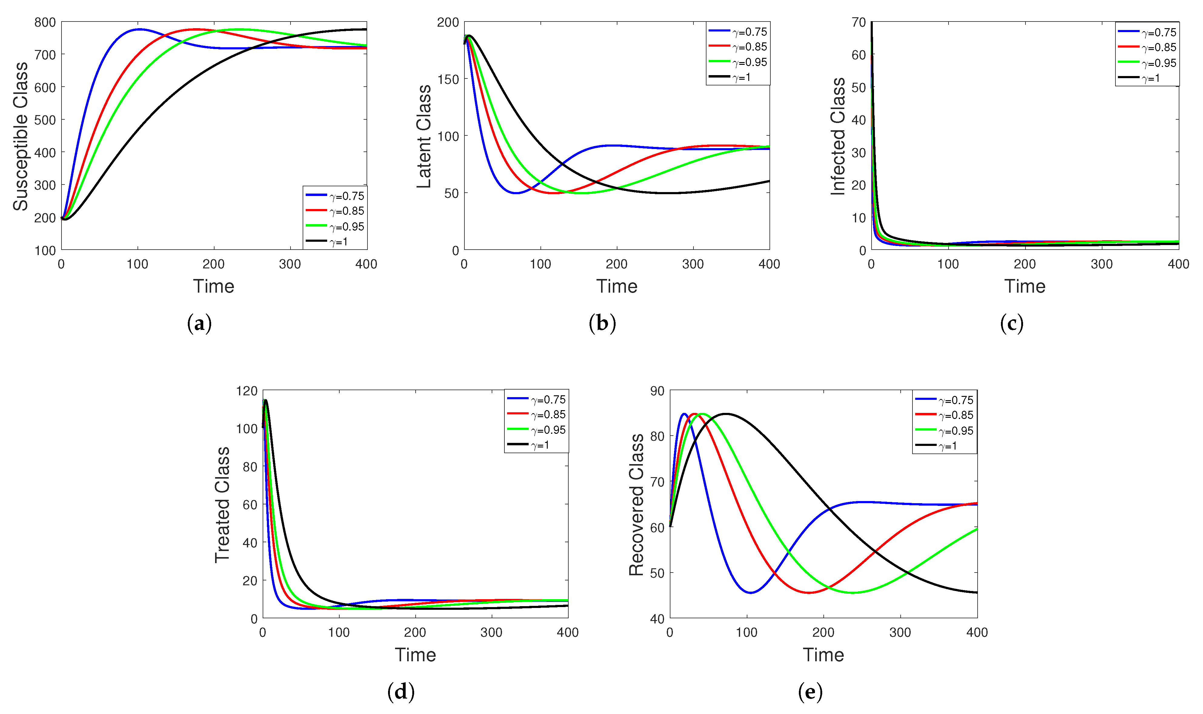
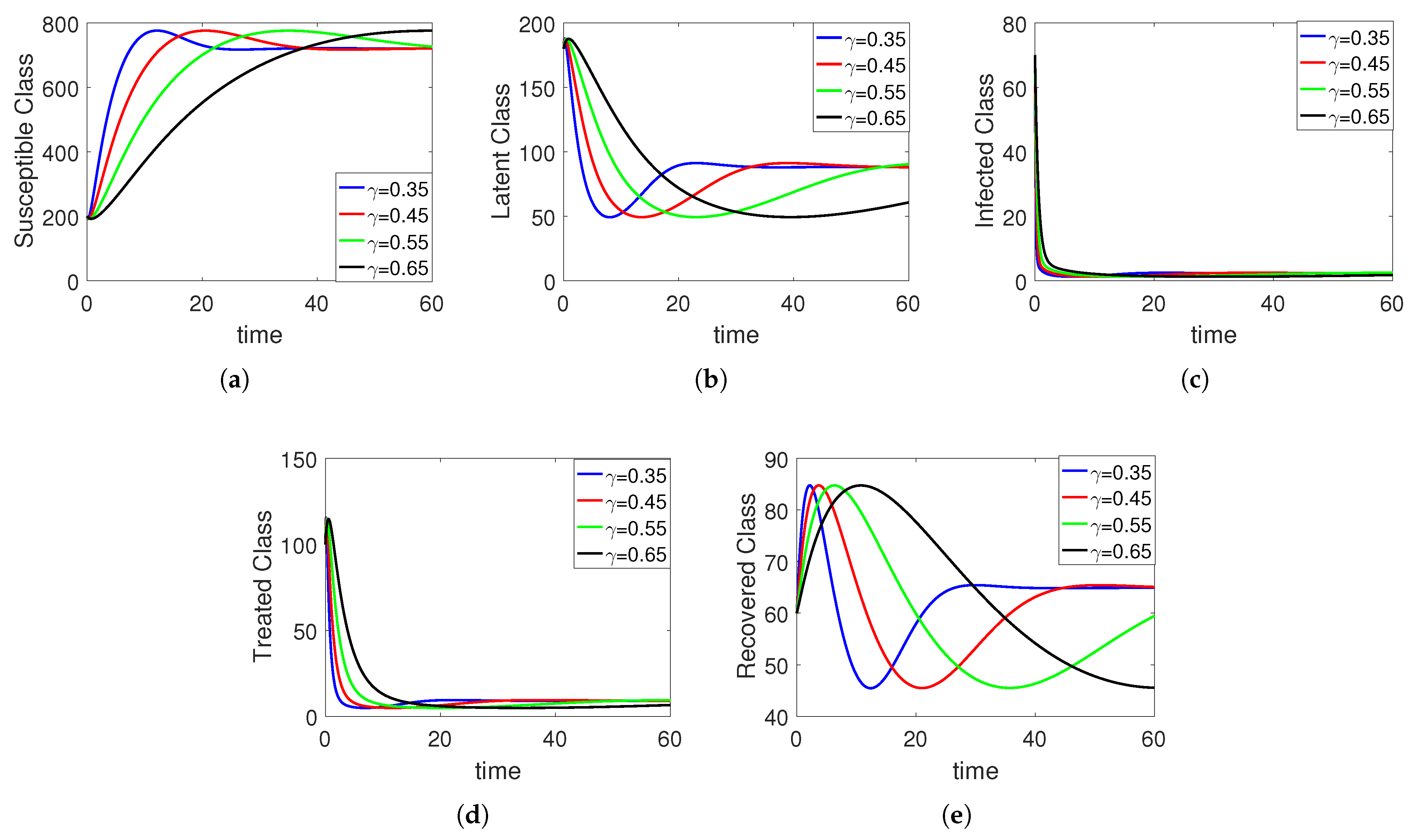
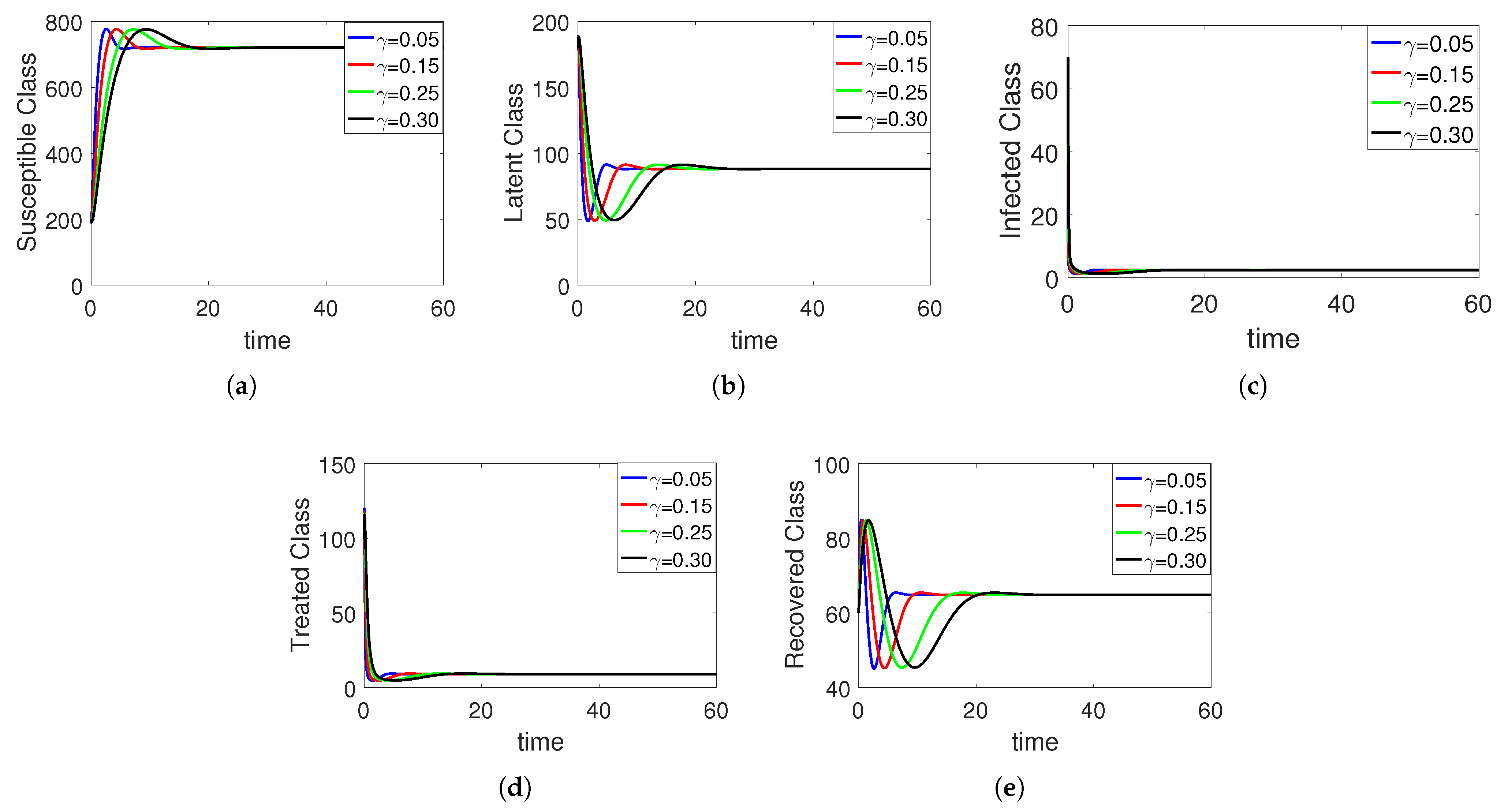
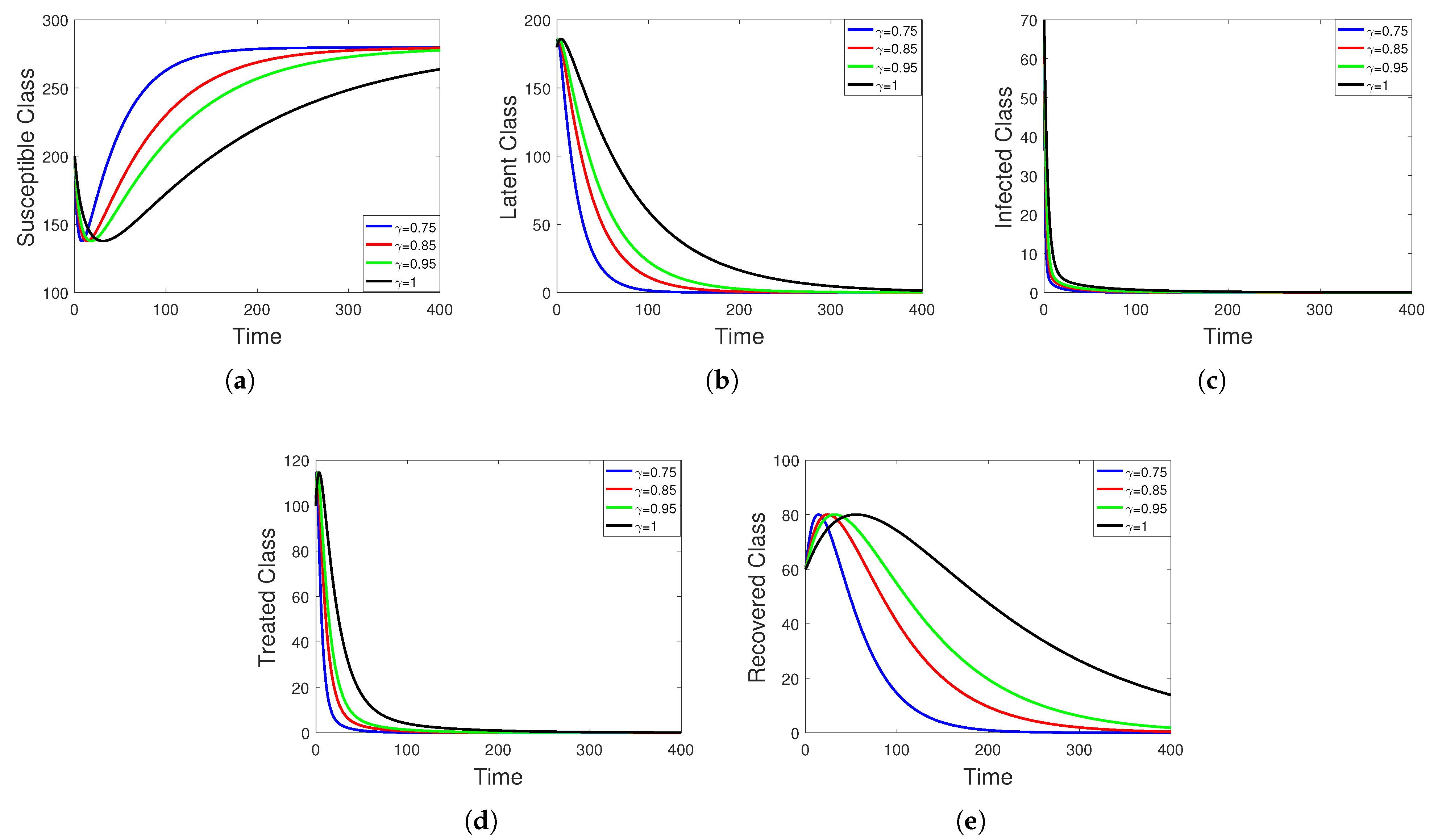
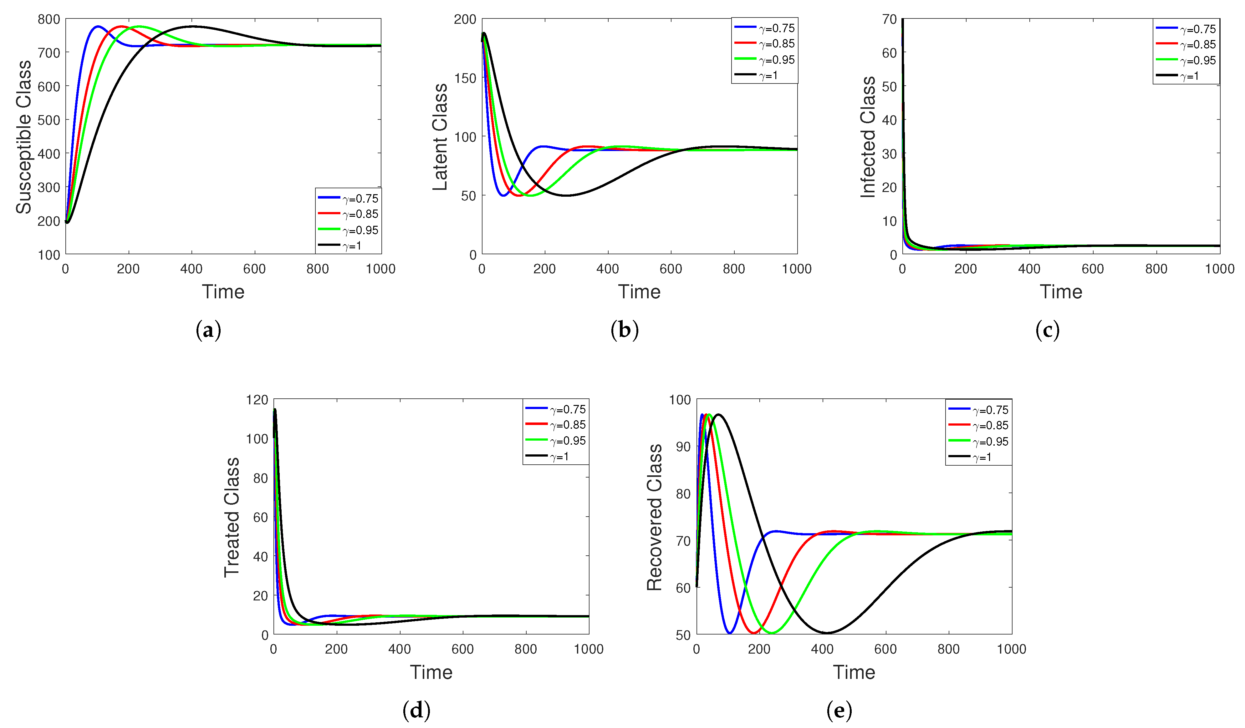
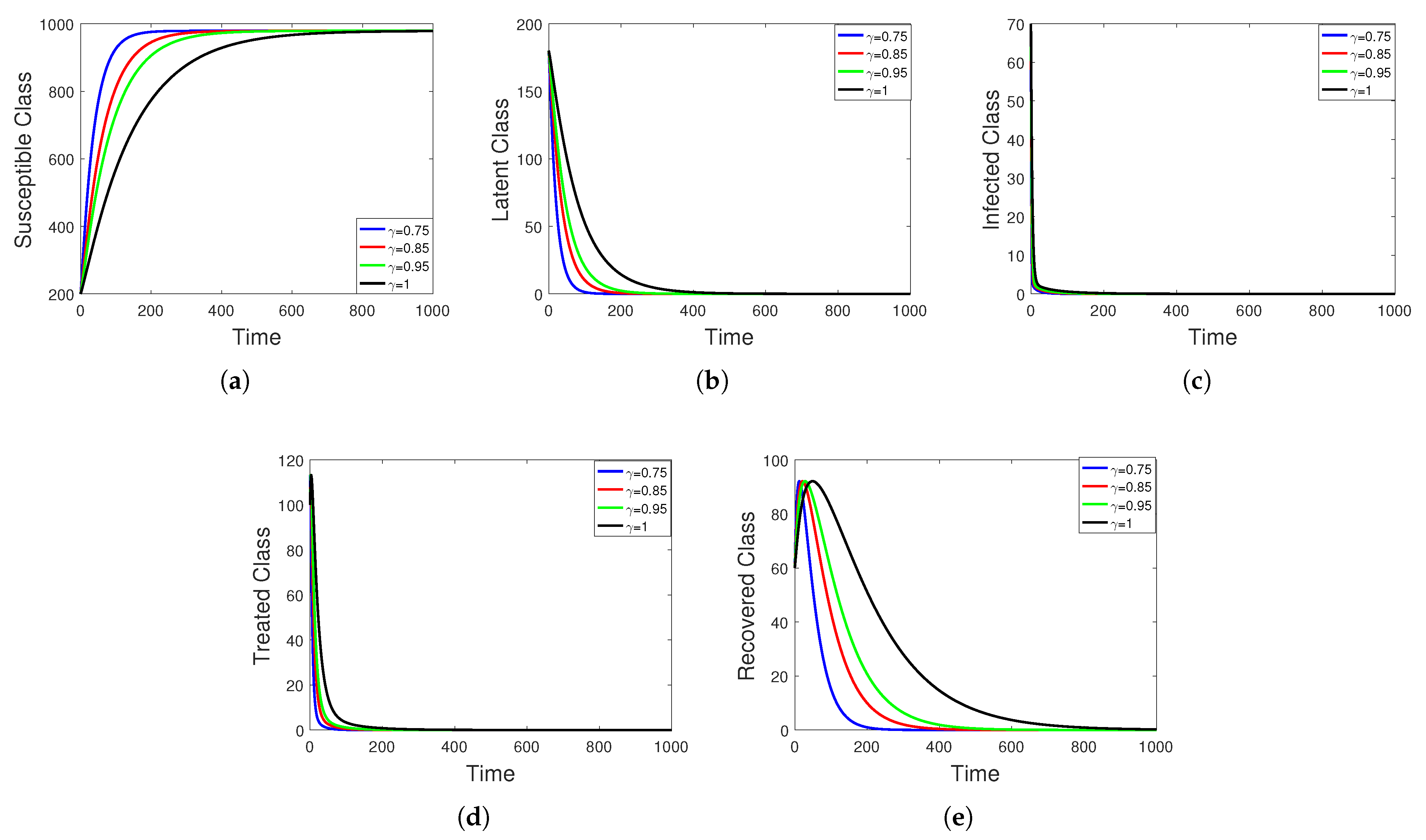
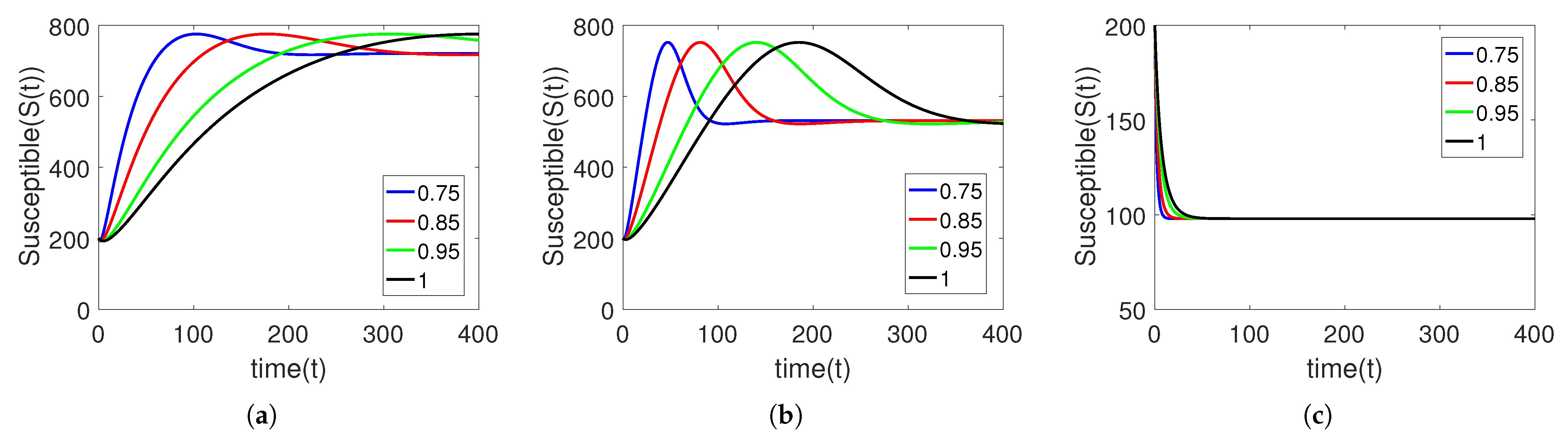
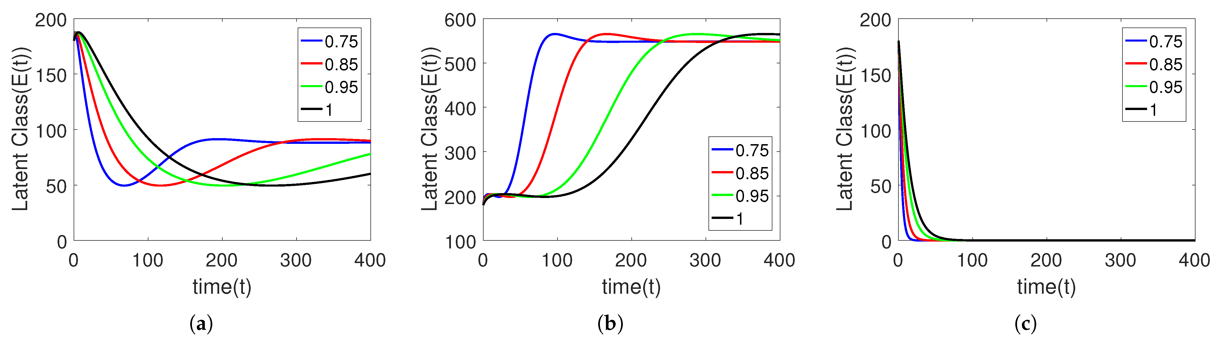
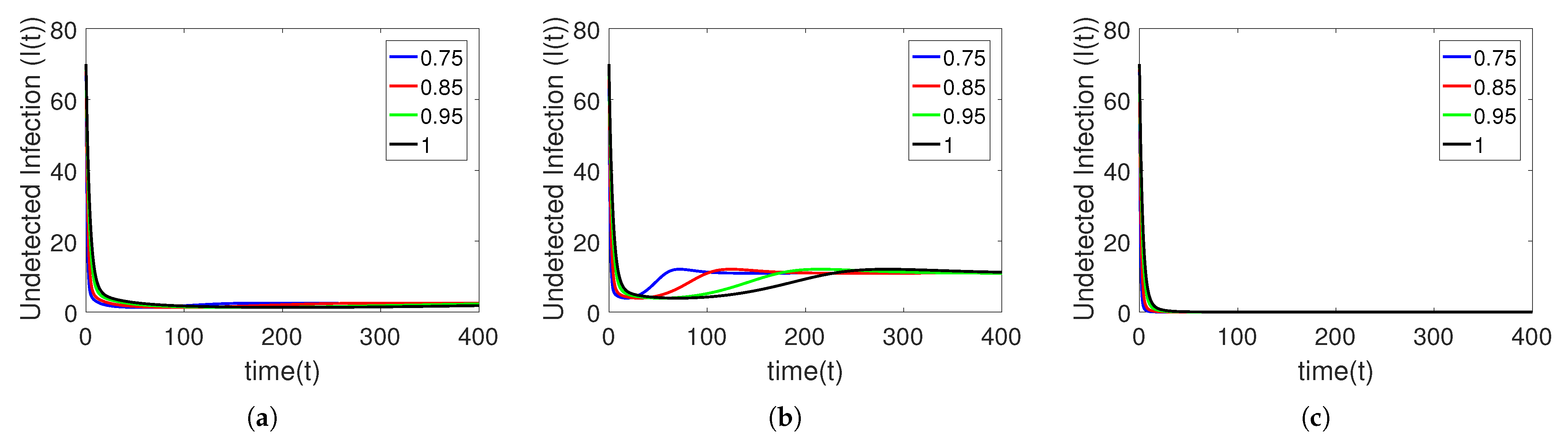
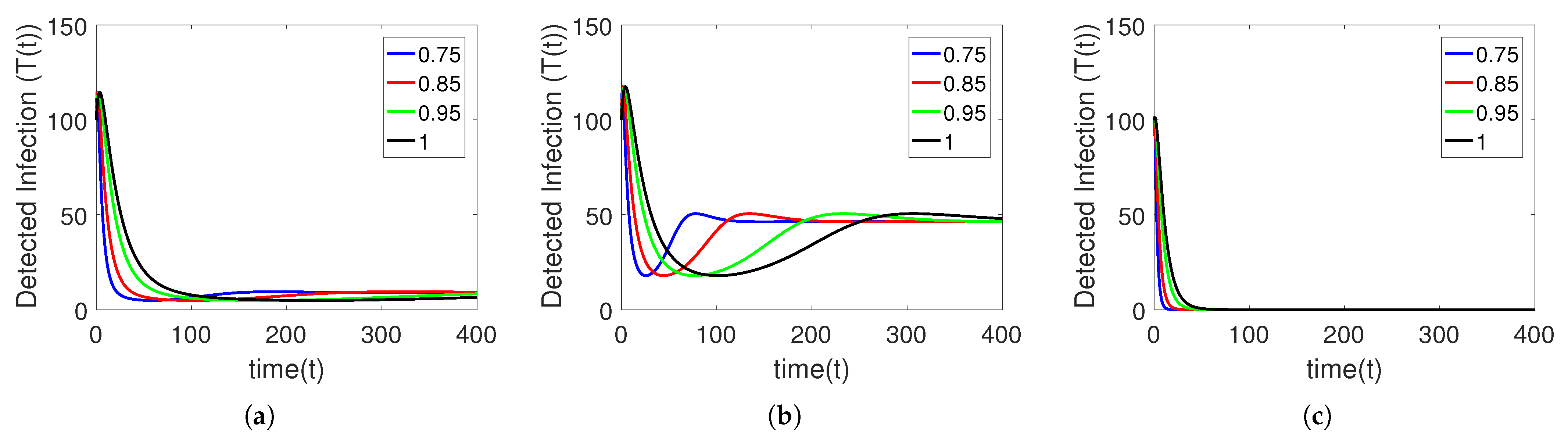
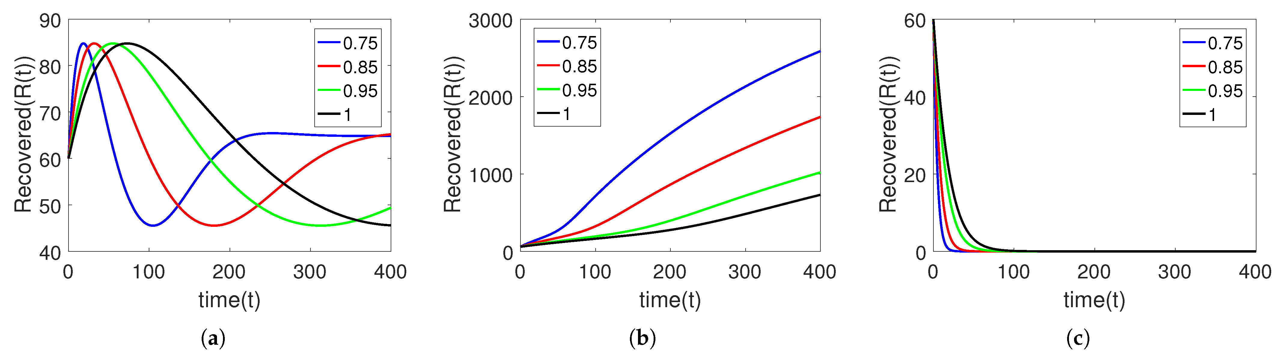
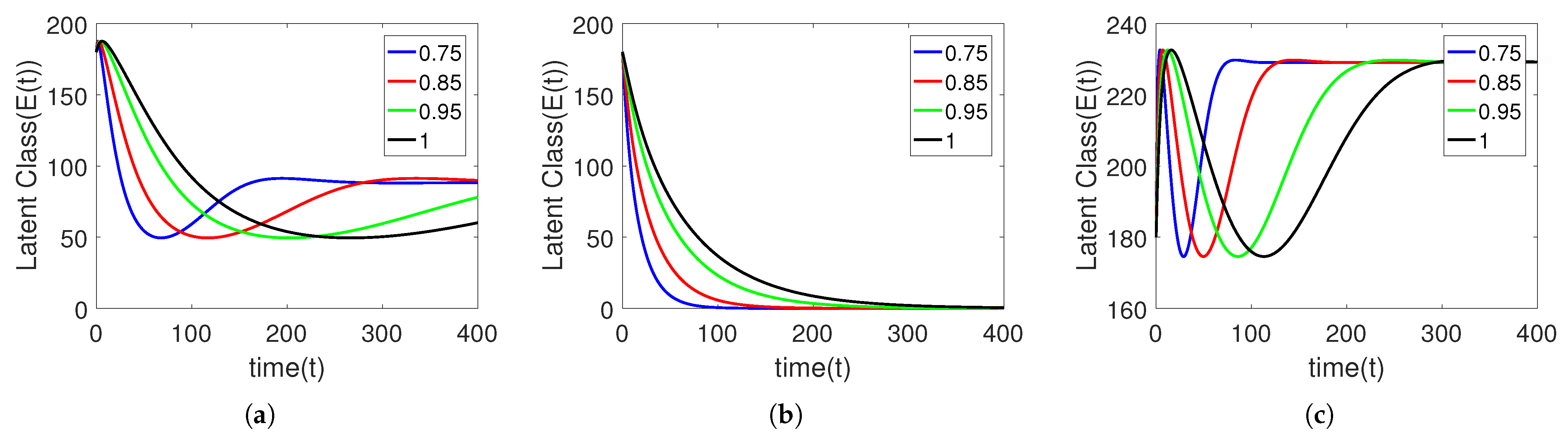
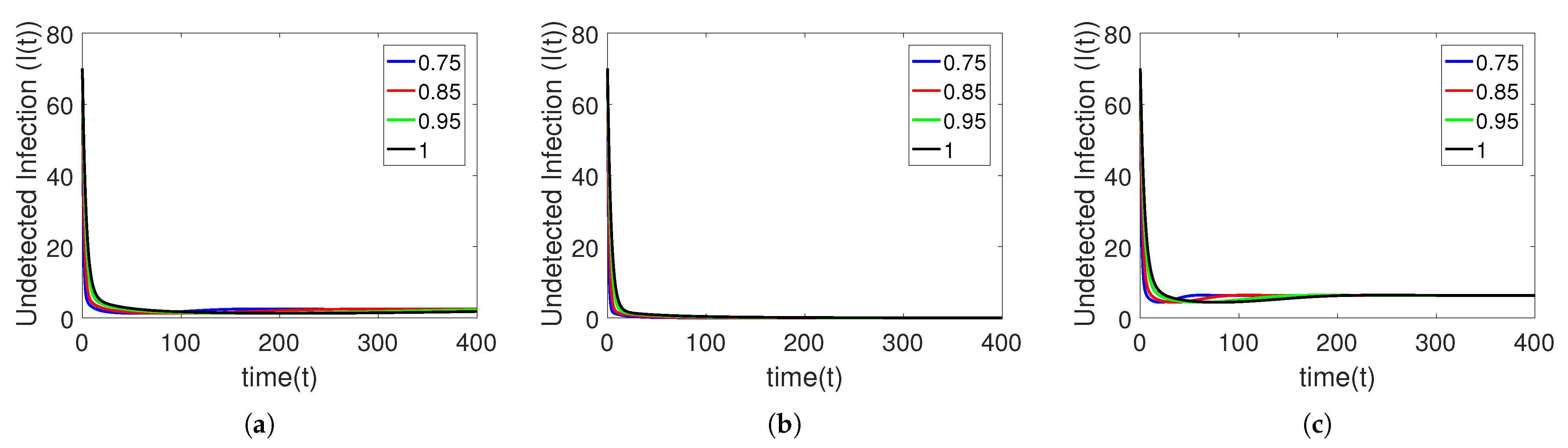
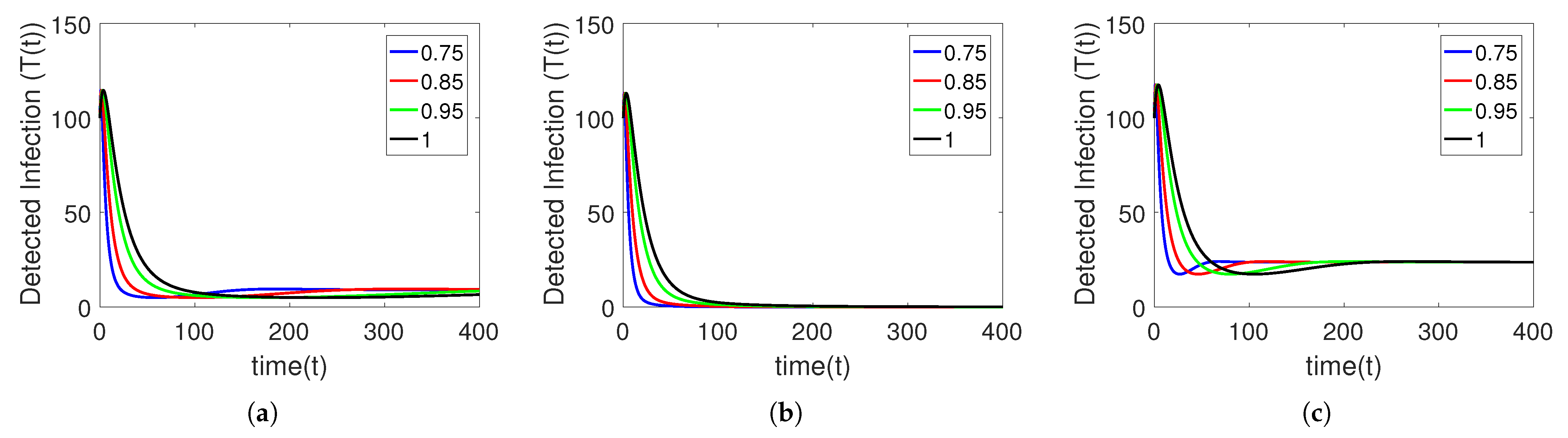
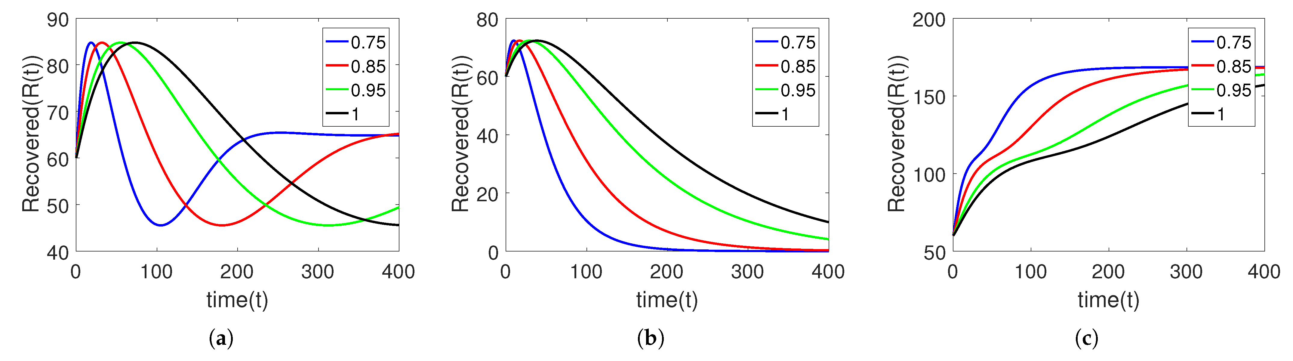
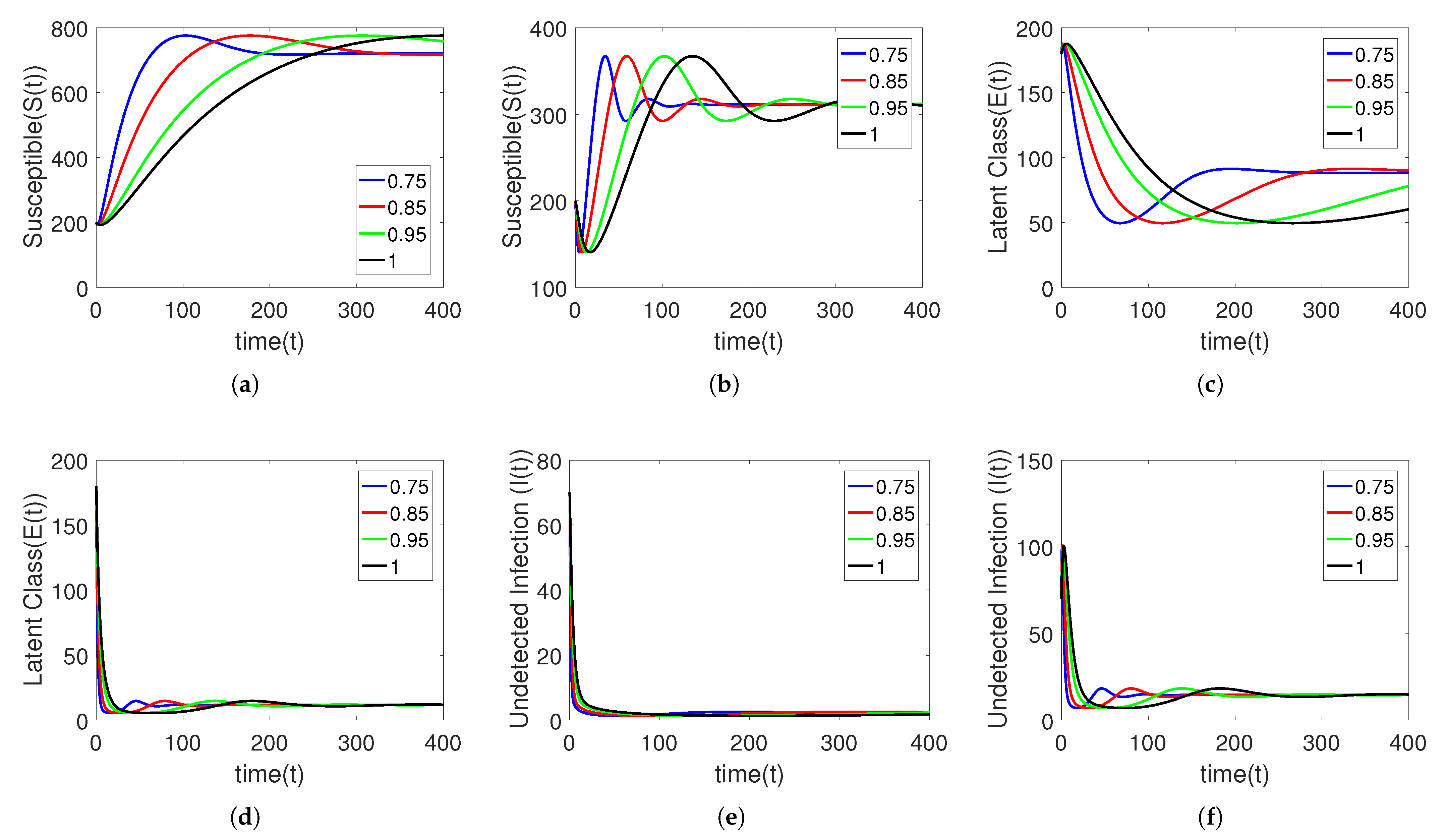
5. Numerical Simulation

Now, we show the dynamical behavior of the proposed disease model by numerical simulation in the sense of the Caputo fractional operator. Furthermore, model (2) is for the effect of awareness on controlling TB. The established numerical scheme of the Laplace–Adomian decomposition technique (LADM) is applied for the approximate solution of the considered problem.

Table 2. Parametric values of the proposed model.

Parameter	Description	Baseline Value	Source
$\lambda$	Rate of recruitment	14	Assumed
$\zeta$	Natural death rate	0.0143	[33]
$\alpha$	Rate of effective contact	Variable	Assumed
$\beta$	Rate of reactivation	0.005	[33]
$\mathrm{\Phi }$	Detection rate	0.25	[34]
$\mathrm{\Psi },r$	Rates of Recovery	0.01, 0.35	Assumed
c	Portion of freshly infected people with latent TB	0.75	[33]
$\rho ,\Delta$	Death rates due to disease	0.08, 0.1	[35]
v	Modification parameter	0.39	Assumed
q	Treatment adherence level	$(0,1)$	Assumed
p	Level of Awareness	$(0,1)$	Assumed

provides the parameter values for simulations that are taken from [14].

The initial densities of all compartments are as follows:

$\mathbb{S}\left(0\right)=200,\mathbb{E}\left(0\right)=180,\mathbb{I}\left(0\right)=70,\mathbb{T}\left(0\right)=100,\mathbb{R}\left(0\right)=60$.

The data are taken from [14], and we further proceed for simulations on different fractional orders. It is clear from these plots that the solution curves of the considered system will converge to the no-disease uniform state with the passage of time.

The graphical view of all compartments is tested for different fractional orders, showing the sensitivity of the fractional parameter. Firstly, the agents are tested on $\gamma =0.75,0.85,0.95,1$ from Figure 1a–e, in which the recovery cases are increased and, consequently, the number of susceptible individuals is increased and then becomes stable. The increase is more on high fractional orders and lower on low fractional orders. The exposed class or latently infected stages decrease and then move up toward stability while the other two classes of undetected infectious and detected infectious cases are controlled and totally decay.

A graphical view of all compartments is shown in Figure 2a–e for another set of fractional orders $\gamma$ = 0.35, 0.45, 0.55, 0.65 to check the sensitivity of the fractional order parameters. Here the same dynamics are again simulated, but this time the time taken is less than the previous one, so we conclude that stability and convergence may be achieved quickly on small fractional orders.

Further, the graphical representation of the compartments is presented in Figure 3a–e for another set of fractional orders $\gamma$ = 0.01, 0.15, 0.25, 0.30 to check the sensitivity of small fractional order parameters. We observe the same dynamics of the compartmental classes, but this time the time taken is much less than the previous one, so we conclude that stability and convergence may be achieved quickly for small fractional orders.

Presented in Figure 4a–e is a graphical representation of the compartments for another set of fractional orders $\gamma =0.75,0.85,0.95,1$ to check the sensitivity of the recruitment rate parameter $A=4$.

Next, the graphical view of all compartments is shown in Figure 5a–e on another set of fractional orders $\gamma$ = 0.75, 0.85, 0.95, 1 to check the sensitivity of two parameters $p=0.6$ and $q=0.6$. Increasing the values of these two parameters will lead to quick stability.

The graphical view of all compartments is shown in Figure 6a–e on another set of fractional orders $0.75,0.85,0.95,1$ to check the sensitivity of two parameters, $p=0.8$ and $q=0.8$. Increasing the values of these two parameters will lead to quick stability.

Sensitivity Analysis

In this subsection we perform the sensitivity of different parameters to show the effect on the dynamics of the proposed model. We test $\eta ,\beta ,\alpha$ for the sensitivity related to the dynamics of each compartment Figure 7, Figure 8, Figure 9, Figure 10, Figure 11, Figure 12, Figure 13, Figure 14, Figure 15, Figure 16, Figure 17 and Figure 18.

6. Conclusions

In this manuscript, we have successfully examined the fractional model for tuberculosis (TB) with five compartments in the sense of the fractional operator of power singular kernel law called the Caputo derivative. The dynamics have been generalized with the extra degree of choices and tested on four different fractional orders along with a comparison with an integer order derivative. By increasing the order of the derivative, the curves converge to their natural order. On small fractional orders, both the detected and undetected infectious cases converge quickly, and vice versa. The considered TB dynamical model was also checked for a unique solution and the existence of the said solution by the application of fixed point theory. The solution of the proposed model is obtained in series form by applying the decomposition technique of the Laplace transformation. In the said technique, the non-linear terms are treated by the Adomian polynomial. In the numerical simulation section, the convergence and stability of the proposed model are verified. All the curves are stable and convergent to their equilibrium points and also to the natural order. Such type of analysis provides the extra information lying between two different integers in the form of a continuous spectrum along with awareness of the TB infection. The whole density of each compartment is achieved by the generalization of the derivative. operator and make the non-differentiable functions into derivable ones. Such an analysis provides the whole spectrum of each quantity in a continuous form, which is very helpful for the inside dynamics lying between 0 and 1.

References

1. Morse, D.; Brothwell, D.R.; Ucko, P.J. Tuberculosis in ancient Egypt. Am. Rev. Respir. Dis. 1964, 90, 524–541. [Google Scholar] [PubMed]
2. Chakaya, J.; Khan, M.; Ntoumi, F.; Aklillu, E.; Fatima, R.; Mwaba, P.; Zumla, A. Global Tuberculosis Report 2020–Reflections on the Global TB burden, treatment and prevention efforts. Int. J. Infect. Dis. 2021, 113, S7–S12. [Google Scholar] [CrossRef] [PubMed]
3. World Health Organization (WHO). Global Tuberculosis Report 2018; World Health Organization (WHO): Geneva, Switzerland, 2018; Available online: https://apps.who.int/iris/handle/10665/274453 (accessed on 10 July 2020).
4. Centers for Disease Control and Prevention. How TB Spreads. Available online: https://www.cdc.gov/tb/topic/basics/howtbspreads.htm (accessed on 11 March 2016).
5. Li, B.; Liang, H.; He, Q. Multiple and generic bifurcation analysis of a discrete Hindmarsh-Rose model. Chaos Solitons Fractals 2021, 146, 110856. [Google Scholar] [CrossRef]
6. Li, B.; Liang, H.; Shi, L.; He, Q. Complex dynamics of Kopel model with nonsymmetric response between oligopolists. Chaos Solitons Fractals 2022, 156, 111860. [Google Scholar] [CrossRef]
7. Eskandari, Z.; Avazzadeh, Z.; Khoshsiar Ghaziani, R.; Li, B. Dynamics and bifurcations of a discrete-time Lotka–Volterra model using nonstandard finite difference discretization method. Math. Methods Appl. Sci. 2022; early view. [Google Scholar] [CrossRef]
8. Li, B.; Zhang, Y.; Li, X.; Eskandari, Z.; He, Q. Bifurcation analysis and complex dynamics of a Kopel triopoly model. J. Comput. Appl. Math. 2023, 426, 115089. [Google Scholar] [CrossRef]
9. Zhang, J.; Feng, G. Global stability for a tuberculosis model with isolation and incomplete treatment. Comput. Appl. Math. 2015, 34, 1237–1249. [Google Scholar] [CrossRef]
10. Trauera, J.M.; Denholm, J.T.; McBryde, E.S. Construction of a mathematical model for tuberculosis transmission in highly endemic regions of the Asia-pacific. J. Theor. Biol. 2014, 358, 74–84. [Google Scholar] [CrossRef] [Green Version]
11. Al-arydah, M.; Hayes, B.; Mushayabasa, S.; Bhunu, C.; Dimitro, D.; Smith, R. Modelling the impact of treatment on tuberculosis transmission dynamic. Int. J. Biomath. Syst. Biol. 2015, 1, 1–19. [Google Scholar]
12. Bhunu, C.P.; Mushayabasa, S.; Smith, R.J. Assessing the effects of poverty in tuberculosis transmission dynamics. Appl. Math. Model. 2012, 36, 4173–4185. [Google Scholar] [CrossRef]
13. Ullah, I.; Ahmad, S.; ur Rahman, M.; Arfan, M. Investigation of fractional order tuberculosis (TB) model via Caputo derivative. Chaos Solitons Fractals 2021, 142, 110479. [Google Scholar] [CrossRef]
14. Ullah, I.; Ahmad, S.; Zahri, M. Investigation of the effect of awareness and treatment on Tuberculosis infection via a novel epidemic model. Alex. Eng. J. 2023, 68, 127–139. [Google Scholar] [CrossRef]
15. Saifullah, S.; Ali, A.; Irfan, M.; Shah, K. Time-fractional Klein–Gordon equation with solitary/shock waves solutions. Math. Probl. Eng. 2021, 2021, 6858592. [Google Scholar] [CrossRef]
16. Goufo, E.F.D.; Khumalo, M.; Toudjeu, I.T.; Yildirim, A. Mathematical application of a non-local operator in language evolutionary theory. Chaos Solitons Fractals 2020, 131, 109541. [Google Scholar] [CrossRef]
17. Opoku, M.O.; Wiah, E.N.; Okyere, E.; Sackitey, A.L.; Essel, E.K.; Moore, S.E. Stability Analysis of Caputo Fractional Order Viral Dynamics of Hepatitis B Cellular Infection. Math. Comput. Appl. 2023, 28, 24. [Google Scholar] [CrossRef]
18. Huo, H.F.; Dang, S.J.; Li, Y.N. Stability of a two-strain tuberculosis model with general contact rate. In Abstract and Applied Analysis; Hindawi: London, UK, 2010; Volume 2010. [Google Scholar]
19. Ain, Q.T.; Anjum, N.; Din, A.; Zeb, A.; Djilali, S.; Khan, Z.A. On the analysis of Caputo fractional order dynamics of Middle East Lungs Coronavirus (MERS-CoV) model. Alex. Eng. J. 2022, 61, 5123–5131. [Google Scholar] [CrossRef]
20. Kumar, S.; Chauhan, R.P.; Momani, S.; Hadid, S. A study of fractional TB model due to mycobacterium tuberculosis bacteria. Chaos Solitons Fractals 2021, 153, 111452. [Google Scholar] [CrossRef]
21. Adnan Ali, A.; Shah, Z.; Kumam, P. Investigation of a time-fractional covid-19 mathematical model with singular kernel. Adv. Contin. Discret. Model. 2022, 2022, 34. [Google Scholar] [CrossRef]
22. Ahmad, S.; Ullah, A.; Akgül, A.; De la Sen, M. A study of fractional order Ambartsumian equation involving exponential decay kernel. AIMS Math. 2021, 6, 9981–9997. [Google Scholar] [CrossRef]
23. Jin, F.; Qian, Z.S.; Chu, Y.M.; ur Rahman, M. On nonlinear evolution model for drinking behavior under Caputo-Fabrizio derivative. J. Appl. Anal. Comput. 2022, 12, 790–806. [Google Scholar] [CrossRef]
24. Doungmo Goufo, E.F. Chaotic processes using the two-parameter derivative with non-singular and non-local kernel: Basic theory and applications. Chaos Interdiscip. J. Nonlinear Sci. 2016, 26, 084305. [Google Scholar] [CrossRef] [PubMed]
25. Kanno, R. Representation of random walk in fractal space-time. Phys. A Stat. Mech. Its Appl. 1998, 248, 165–175. [Google Scholar] [CrossRef]
26. Chen, W.; Sun, H.; Zhang, X.; Korošak, D. Anomalous diffusion modeling by fractal and fractional derivatives. Comput. Math. Appl. 2010, 59, 1754–1758. [Google Scholar] [CrossRef] [Green Version]
27. Sun, H.; Meerschaert, M.M.; Zhang, Y.; Zhu, J.; Chen, W. A fractal Richards’ equation to capture the non-Boltzmann scaling of water transport in unsaturated media. Adv. Water Resour. 2013, 52, 292–295. [Google Scholar] [CrossRef] [Green Version]
28. Atangana, A. Fractal-fractional differentiation and integration: Connecting fractal calculus and fractional calculus to predict complex system. Chaos Solitons Fractals 2017, 102, 396–406. [Google Scholar] [CrossRef]
29. Shojaeizadeh, T.; Mahmoudi, M.; Darehmiraki, M. Optimal control problem of advection-diffusion-reaction equation of kind fractal-fractional applying shifted Jacobi polynomials. Chaos Solitons Fractals 2021, 143, 110568. [Google Scholar] [CrossRef]
30. Xu, C.; Saifullah, S.; Ali, A. Theoretical and numerical aspects of Rubella disease model involving fractal fractional exponential decay kernel. Results Phys. 2022, 34, 105287. [Google Scholar] [CrossRef]
31. Miller, K.S.; Ross, B. An Introduction to the Fractional Calculus and Fractional Differential Equations; Wiley: Hoboken, NJ, USA, 1993. [Google Scholar]
32. Biazar, J. Solution of the epidemic model by Adomian decomposition method. Appl. Math. Comput. 2006, 173, 1101–1106. [Google Scholar] [CrossRef]
33. Khan, A.M.; Ahmad, M.; Ullah, S.; Farooq, M.; Gul, T. Modelling the transmission dynamics of tuberculosis in Khyber Pakhtunkhwa Pakistan. Adv. Mech. Eng. 2019, 11, 1–13. [Google Scholar] [CrossRef] [Green Version]
34. Egonmwan, A.O.; Okuonghae, D. Analysis of a mathematical model for tuberculosis with diagnosis. J. Appl. Math. Comput. 2019, 59, 129–162. [Google Scholar] [CrossRef]
35. Yang, Y.; Li, J.; Ma, Z.; Liu, L. Global stability of two models with incomplete treatment for tuberculosis. Chaos Solitons Fractals 2010, 43, 79–85. [Google Scholar] [CrossRef]
Figure 1. A graphic view of all five compartments (ae) of human society for different arbitrary orders γ = 0.75, 0.85, 0.95, 1 for initial data and time duration.
Fractalfract 07 00300 g001
Figure 2. A graphic view of all five agents (ae) of human society on different arbitrary orders γ = 0.35, 0.45, 0.55, 0.65 for initial data and time duration.
Fractalfract 07 00300 g002
Figure 3. A graphic view of all five agents (ae) of human society on different arbitrary orders γ = 0.05, 0.15, 0.25, 0.30 for initial data and time duration.
Fractalfract 07 00300 g003
Figure 4. A graphical representation of human society (ae) for different arbitrary orders γ = 0.75, 0.85, 0.95, 1 for initial data and time duration of TB model by taking the value of λ = 4 .
Fractalfract 07 00300 g004
Figure 5. A graphical representation of human compartments (ae) on different arbitrary orders γ = 0.75, 0.85, 0.95, 1 for initial data and time duration for the TB model by taking the value of p = q = 0.6 .
Fractalfract 07 00300 g005
Figure 6. Simulations of the five classes (ae) of the proposed model for different arbitrary orders γ = 0.75 , 0.85 , 0.95 , 1 for initial data and time duration for the TB model by taking the value of p = q = 0.8 .
Fractalfract 07 00300 g006
Figure 7. Graphical view (ac) of a susceptible individual on different arbitrary orders γ = 0.75 , 0.85 , 0.95 , 1 for initial data and time duration for TB model by taking the value of η = 0.0143 , 0.143 , 1.143 .
Fractalfract 07 00300 g007
Figure 8. Graphical view (ac) of Latent class on different arbitrary orders γ = 0.75 , 0.85 , 0.95 , 1 for initial data and time duration for TB model by taking the value of η = 0.0143 , 0.143 , 1.143 .
Fractalfract 07 00300 g008
Figure 9. Graphical view (ac) of Undetected infected class on different arbitrary orders γ = 0.75, 0.85, 0.95, 1 for initial data and time duration for TB model by taking the value of η = 0.0143, 0.143, 1.143.
Fractalfract 07 00300 g009
Figure 10. Graphical view (ac) of Detected infected class on different arbitrary orders γ = 0.75 , 0.85 , 0.95 , 1 for initial data and time duration for TB model by taking the value of η = 0.0143 , 0.143 , 1.143 .
Fractalfract 07 00300 g010
Figure 11. Graphical view (ac) of Recovered class on different arbitrary orders γ = 0.75 , 0.85 , 0.95 , 1 for initial data and time duration for TB model by taking the value of η = 0.0143 , 0.143 , 1.143 .
Fractalfract 07 00300 g011
Figure 12. Graphical view (ac) of Susceptible class on different arbitrary orders γ = 0.75 , 0.85 , 0.95 , 1 for initial data and time duration for TB model by taking the value of β = 0.75 , 0.075 , 1.75 .
Fractalfract 07 00300 g012
Figure 13. Graphical view (ac) of Latent class on different arbitrary orders γ = 0.75 , 0.85 , 0.95 , 1 for initial data and time duration for TB model by taking the value of β = 0.75 , 0.075 , 1.75 .
Fractalfract 07 00300 g013
Figure 14. Graphical view (ac) of Undetected infected class on different arbitrary orders γ = 0.75, 0.85, 0.95, 1 for initial data and time duration for TB model by taking the value of β = 0.75, 0.075, 1.75.
Fractalfract 07 00300 g014
Figure 15. Graphical view (ac) of the Detected infected class on different arbitrary orders γ = 0.75, 0.85, 0.95, 1 for initial data and time duration for TB model by taking the value of β = 0.75, 0.075, 1.75.
Fractalfract 07 00300 g015
Figure 16. Graphical view (ac) of Recovered class on different arbitrary orders γ = 0.75, 0.85, 0.95, 1 for initial data and time duration for TB model by taking the value of β = 0.75, 0.075, 1.75.
Fractalfract 07 00300 g016
Figure 17. Graphical view (af) of first three classes on different arbitrary orders γ = 0.75 , 0.85 , 0.95 , 1 for initial data and time duration for TB model by taking the value of α = 0.005 , 0.05 , 0.5 .
Fractalfract 07 00300 g017
Figure 18. Graphical view (ad) of last two classes on different arbitrary orders γ = 0.75 , 0.85 , 0.95 , 1 for initial data and time duration for TB model by taking the value of α = 0.005 , 0.5 .
Fractalfract 07 00300 g018