


New Method to Investigate the Impact of Independent Quadratic α-Stable Poisson Jumps on the Dynamics of a Disease under Vaccination Strategy


Abstract
1. Introduction
- •
- : , ; is increasing in and decreasing in ; is increasing in and decreasing in ; and there exists two positive constants , such thatfor all .
- •
- : and follow the uniform continuity property at :

- •
- indicate the left limits of .
- •
- are alternately independent Wiener processes presented on .
- •
- denote the linear diffusion amplitudes; and represent the strengths of quadratic fluctuations.
- •
- are the mutually independent compensator processes associated respectively with the Poisson random measures .
- •
- are independent to .
- •
- are the tempered -stable Lévy measures defined on a measurable set .
- •
- and are -martingales, where
- •
- The tempered -stable Lévy measures are expressed as follows:
- •
- We principally presume that the intensities and are positive continuous functions that meet the following primary criterion::
2. Some Preliminaries and Required Lemmas
3. Long-Run Bifurcation of the Stochastic System (2)
3.1. The Stationarity Case
3.2. The Disappearance Case
4. Numerical Verification
- •
- is an i.i.d. Bernoulli random sequence with the associated distribution .
- •
- and are i.i.d. exponential random variables with the parameter 1, where .
- •
- are i.i.d. uniform random variables.
- •
- is an i.i.d. uniform random sequence.
- •
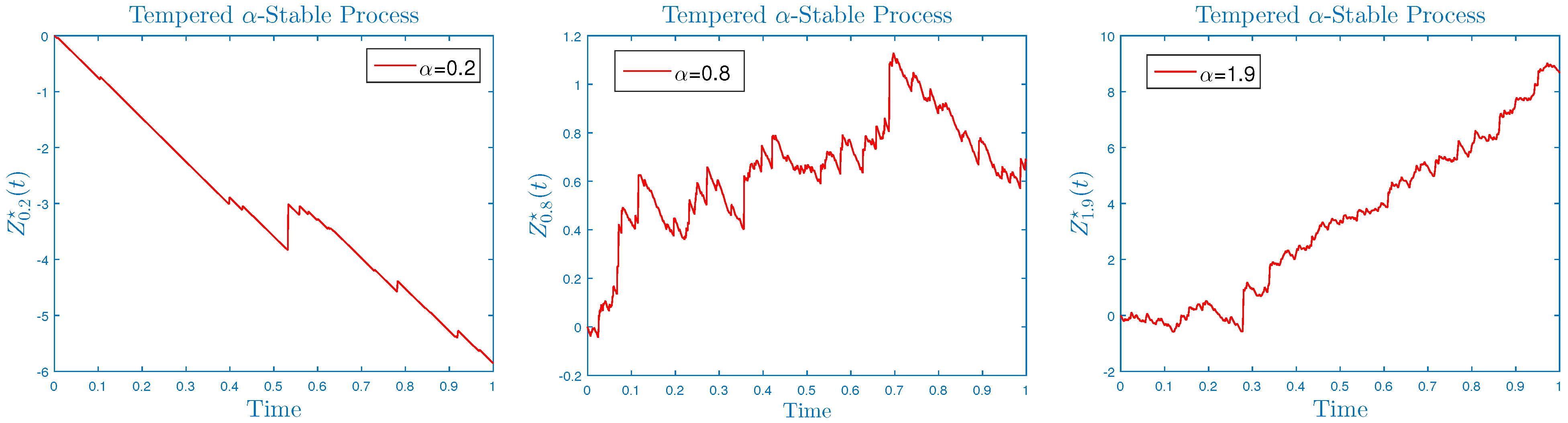
- When , then , for all , where .
- •
- When , then for all where , , andwhere denotes the Riemann zeta function, is the Gamma function, and is the Euler constant.
4.1. First Case:
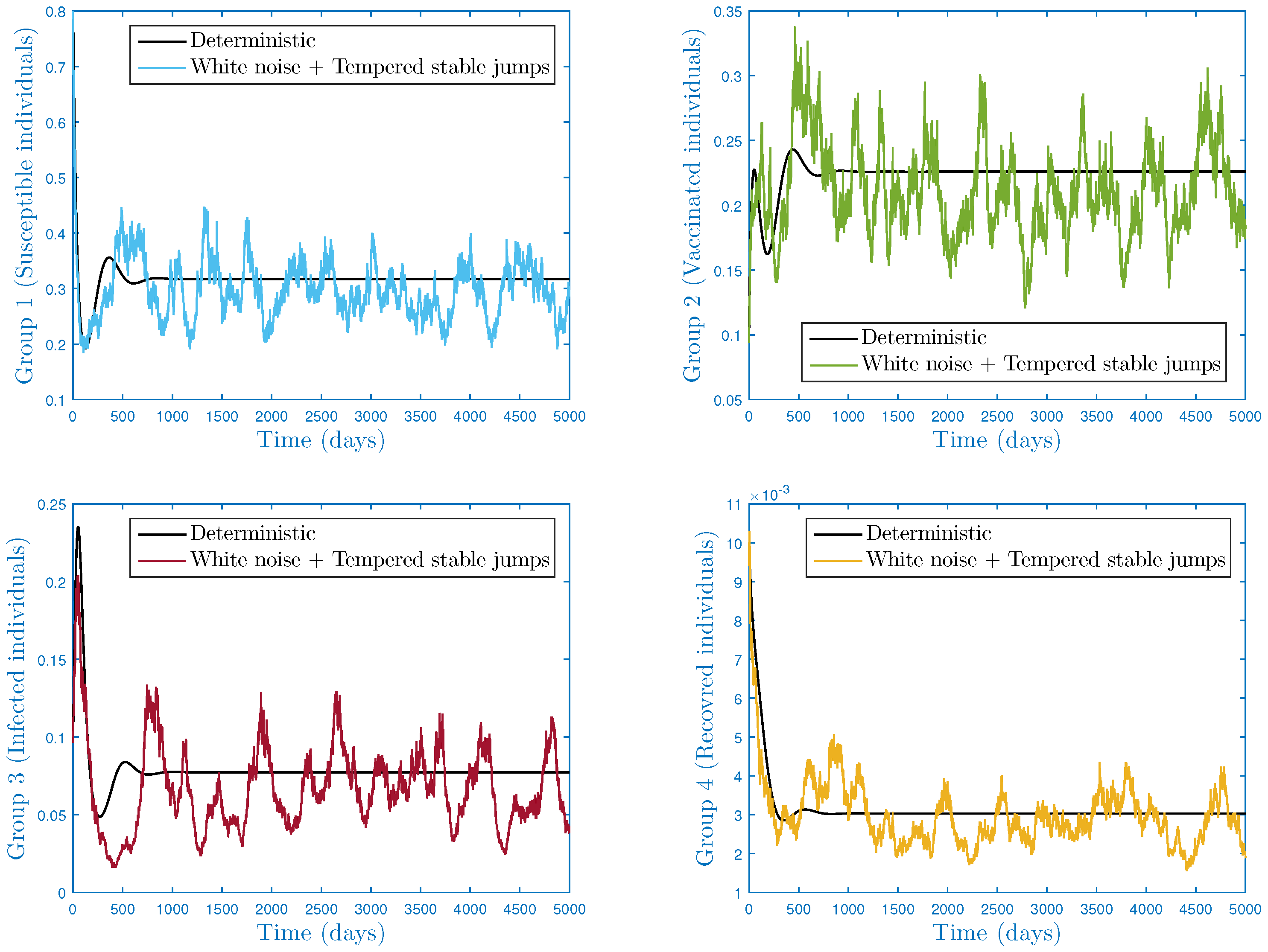
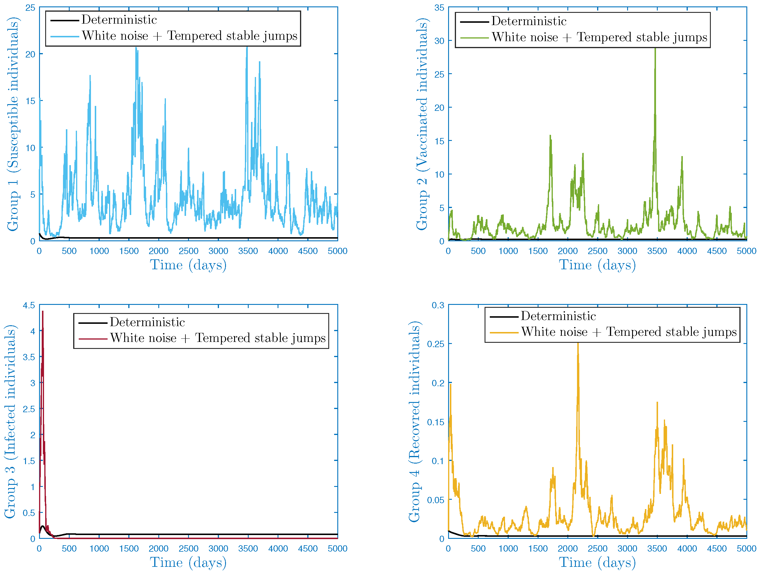
4.1.1. Scenario 1: Stationarity and Permanence
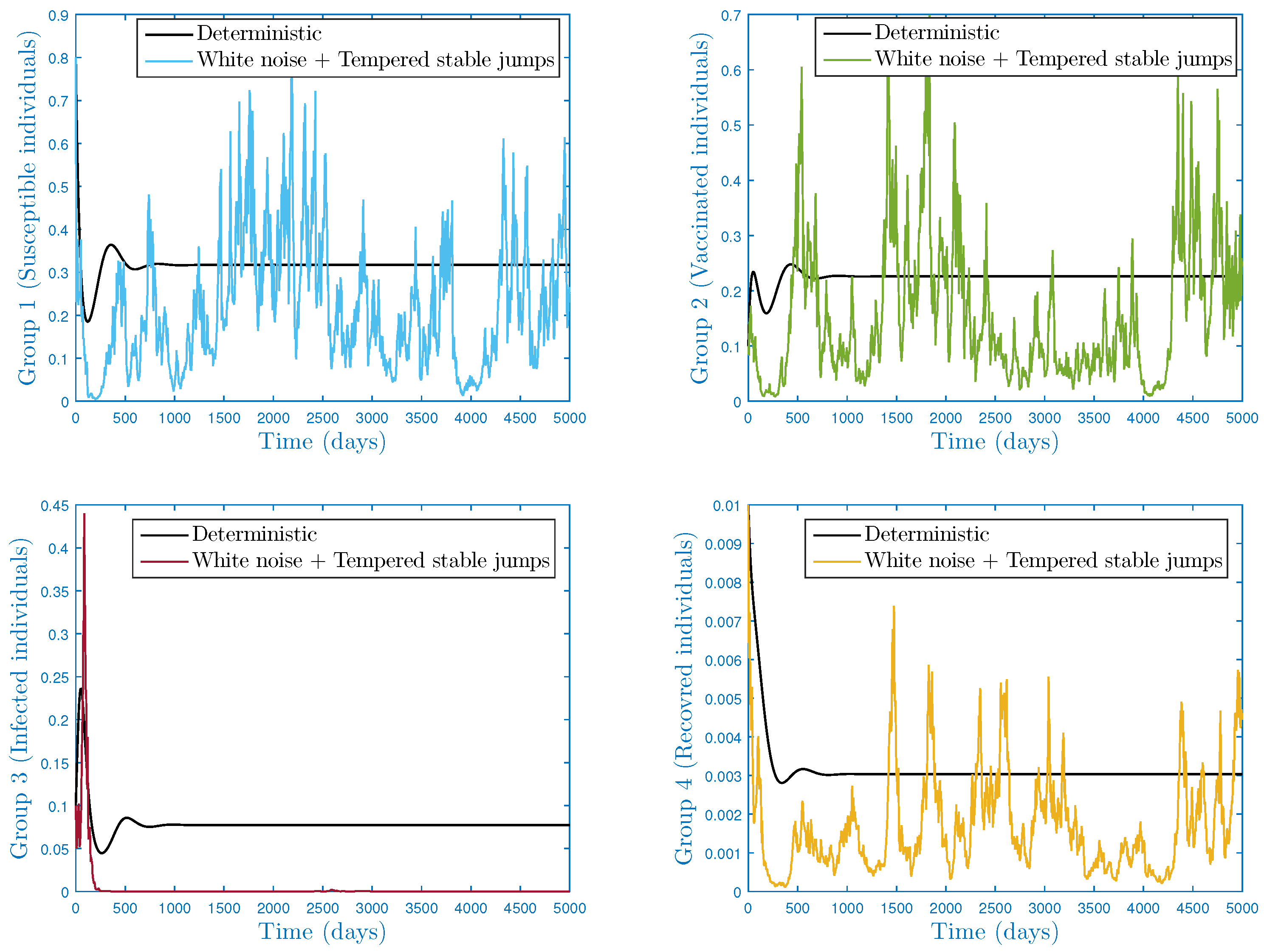
4.1.2. Scenario 2: Extinction
4.2. Second Case:
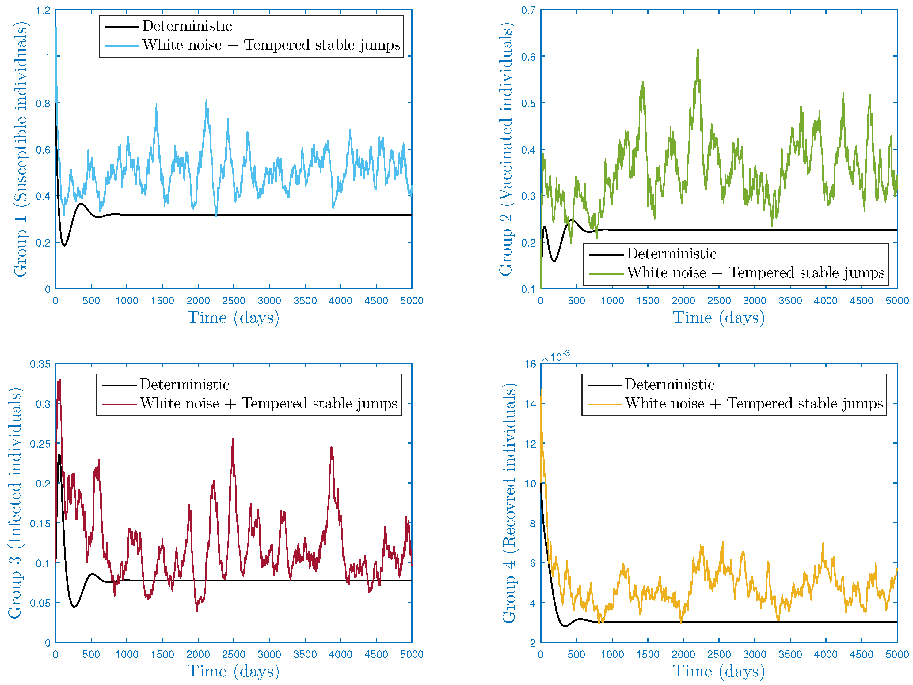
4.2.1. Scenario 1: Stationarity and Permanence
4.2.2. Scenario 2: Extinction
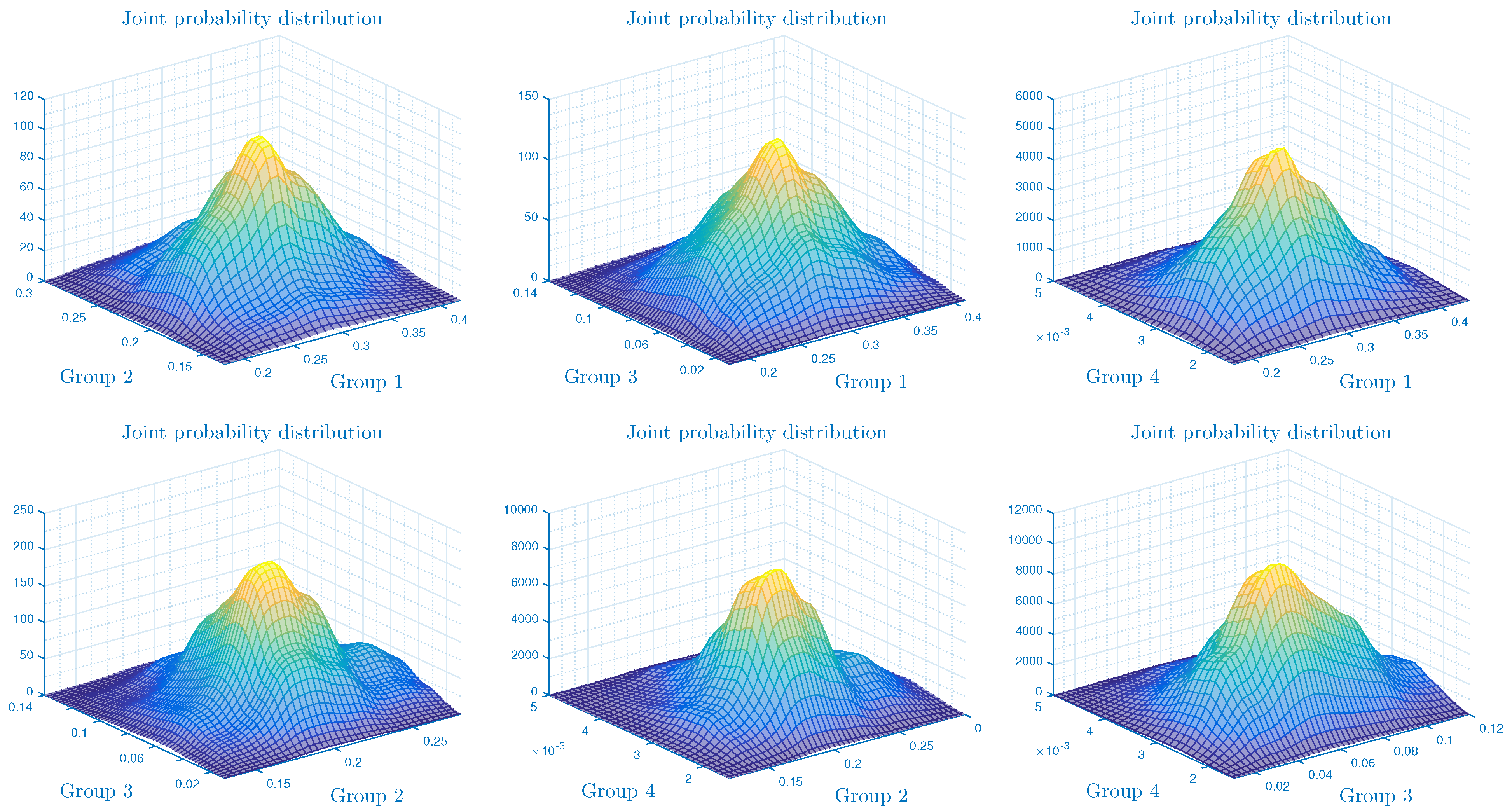
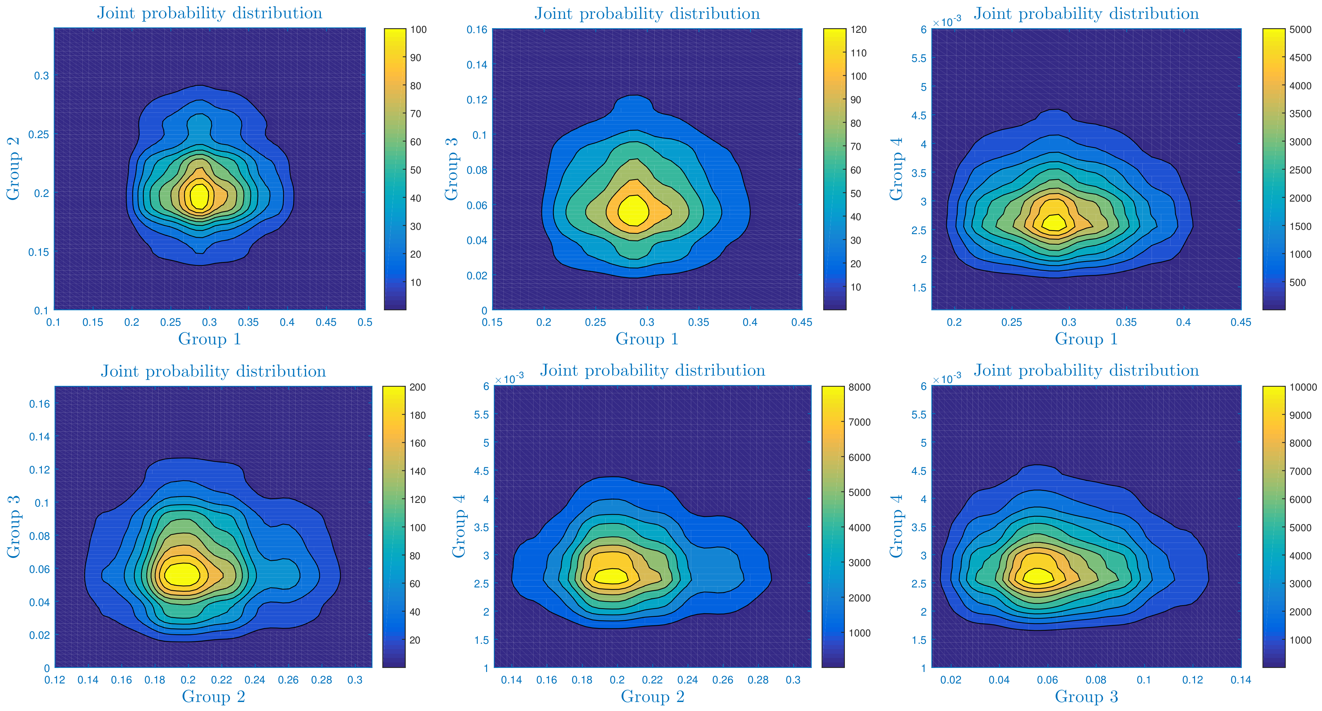
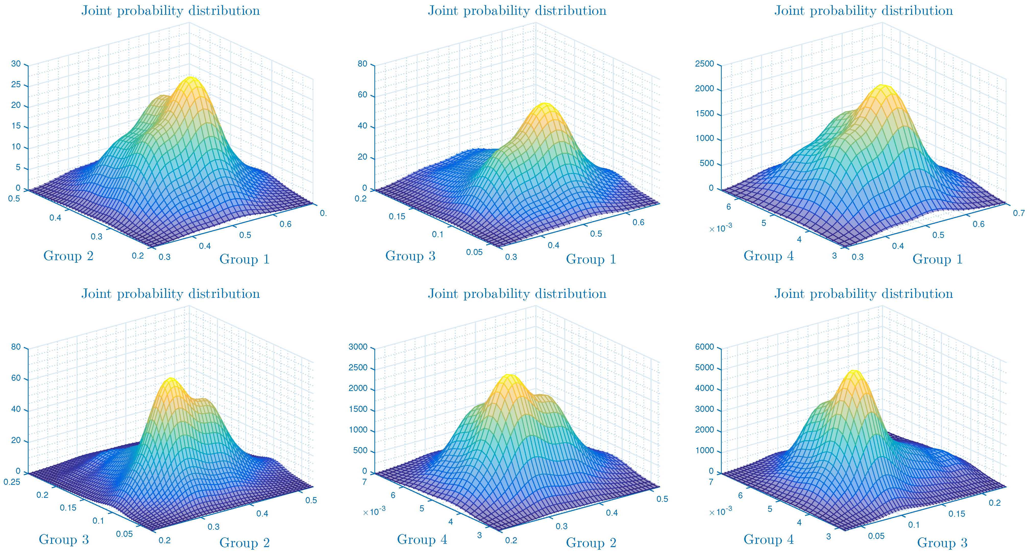
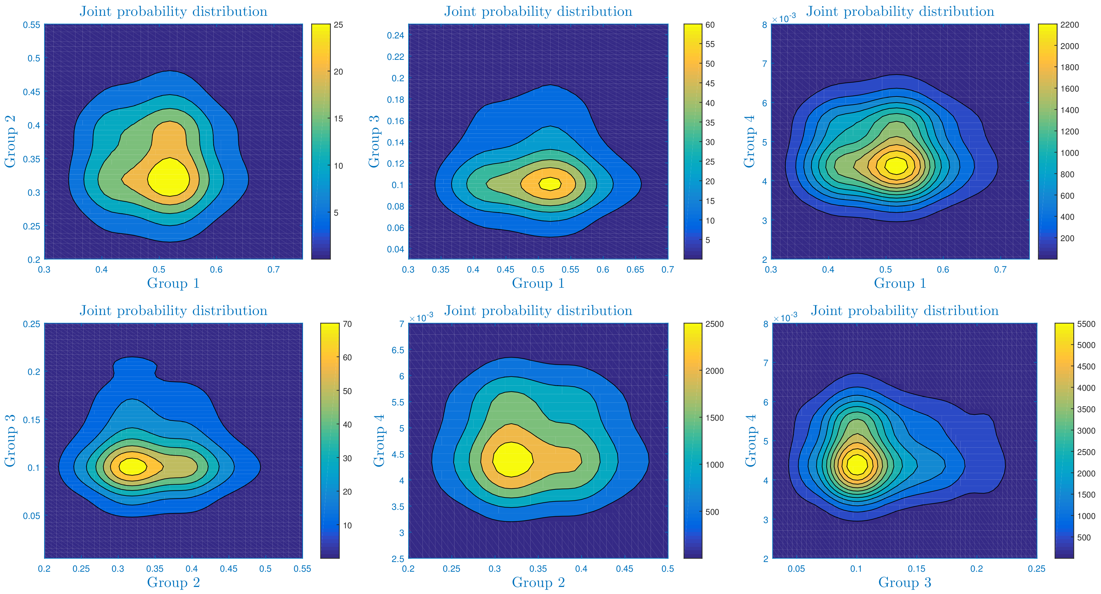
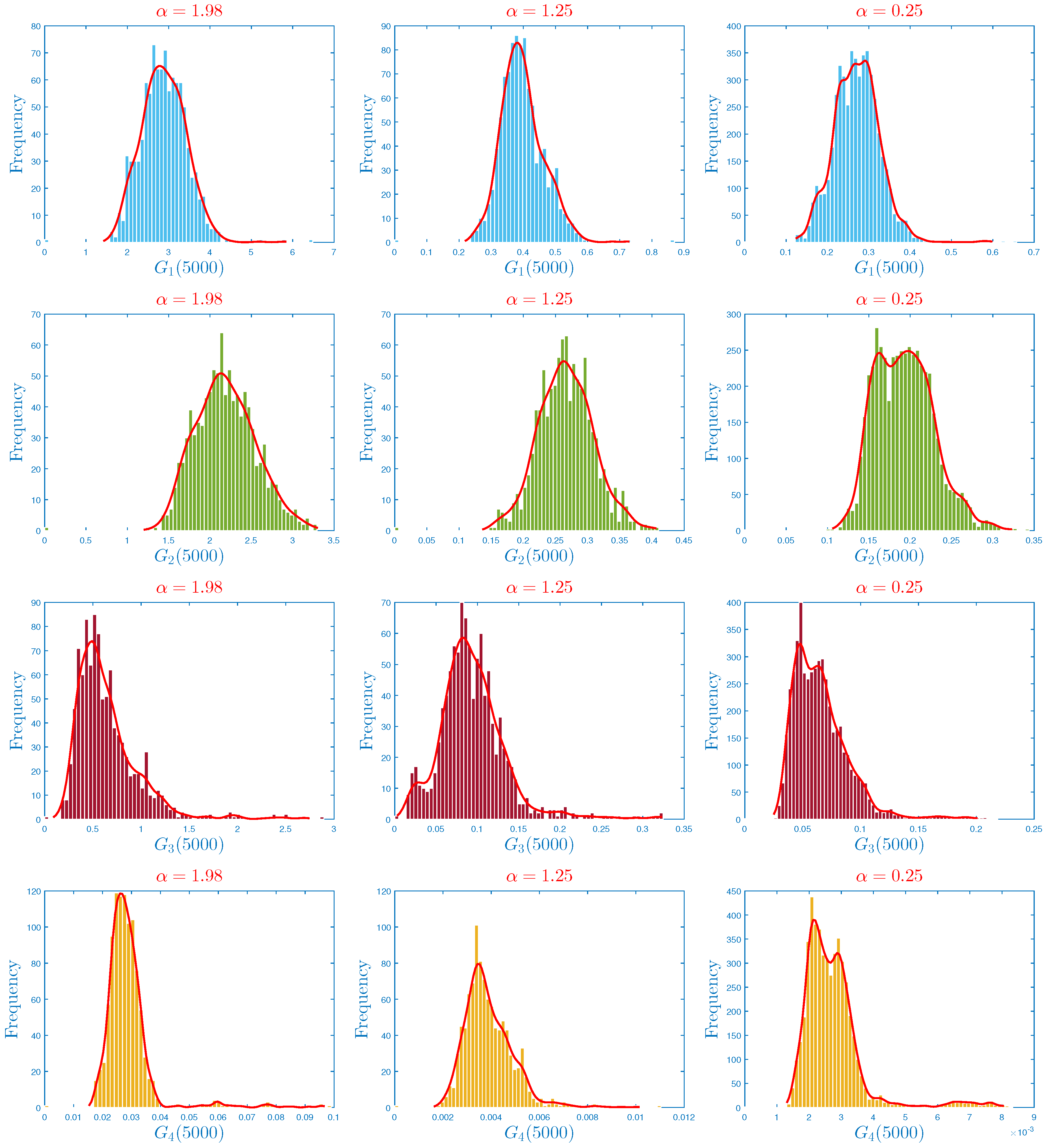
4.3. The Influence of Parameter on the Form of the Probability Density Function
5. Conclusions
- •
- We determined the novel model’s global threshold using some dynamical properties of a two-block boundary system (5) perturbed by quadratic tempered -stable Lévy noises.
- •
- In Theorem 1, we proved a few results related to the stationarity and ergodicity of the system. It is worthy to mention that the analysis of these long-term properties is very significant for the underlying perturbed systems, especially in case of epidemiological models where the ergodicity offers a general idea of the infection permanence.
- •
- In Theorem 2, we studied the extinction case and the weak convergence of susceptible and vaccinated distributions to that of the two-block boundary system (5).
- •
- In the numerical simulation part, we have ensured the accuracy of our threshold. Further, we explored the impact of noise and on the infection’s dynamics. In particular, we showed that jumps have a negative influence on the long-term behavior of the disease in the sense that they lead to complete extinction. Furthermore, it was discovered that parameter had a significant impact on the shape of the stationary distribution.
Author Contributions
Funding
Informed Consent Statement
Data Availability Statement
Conflicts of Interest
Appendix A. Proof of Lemma 4
Appendix B. Proof of Theorem 1
Appendix C. Proof of Theorem 2
References
- Hays, J.N. Epidemics and Pandemics: Their Impacts on Human History; Abc-Clio: Santa Barbara, CA, USA, 2005. [Google Scholar]
- Ministry of Health of Morocco. Available online: www.sante.gov.ma (accessed on 15 November 2022).
- May, R.M. Stability and Complexity in Model Ecosystems; Princeton Landmarks in Biology; Princeton University Press: Princeton, NJ, USA, 2001. [Google Scholar]
- Nair, S. Advanced Topics in Applied Mathematics: For Engineering and the Physical Sciences; Cambridge University Press: Cambridge, UK, 2011. [Google Scholar]
- Kermack, W.O.; McKendrick, A.G. A contribution to the mathematical theory of epidemics. Proc. R. Soc. Math. Phys. Eng. Sci. 1927, 115, 700–721. [Google Scholar]
- Heymann, D.L.; Shindo, N. COVID-19: What is next for public health? Lancet 2020, 395, 542–545. [Google Scholar] [CrossRef] [PubMed]
- Buonomo, B. Effects of information-dependent vaccination behavior on coronavirus outbreak: Insights from a SIRI model. Ric. Mat. 2020, 69, 483–499. [Google Scholar] [CrossRef]
- Harianto, J.; Sari, I.P. Local Dynamics of an SVIR Epidemic Model with Logistic Growth. Cauchy—J. Mat. Murni Dan Apl. 2020, 6, 122–132. [Google Scholar] [CrossRef]
- Horsthemke, W.; Lefever, R. Noise-Induced Transitions: Theory and Applications in Physics, Chemistry, and Biology; Springer: Berlin/Heidelberg, Germany, 1984. [Google Scholar]
- Sabbar, Y.; Yavuz, M.; Ozkose, F. Infection Eradication Criterion in a General Epidemic Model with Logistic Growth, Quarantine Strategy, Media Intrusion, and Quadratic Perturbation. Mathematics 2022, 10, 4213. [Google Scholar] [CrossRef]
- Sabbar, Y.; Kiouach, D.; Rajasekar, S.P.; El-Idrissi, S.E.A. The influence of quadratic Lévy noise on the dynamic of an SIC contagious illness model: New framework, critical comparison and an application to COVID-19 (SARS-CoV-2) case. Chaos Solitons Fractals 2022, 159, 112110. [Google Scholar] [CrossRef]
- Din, A.; Khan, A.; Sabbar, Y. Long-Term Bifurcation and Stochastic Optimal Control of a Triple-Delayed Ebola Virus Model with Vaccination and Quarantine Strategies. Fractal Fract. 2022, 6, 578. [Google Scholar] [CrossRef]
- Khan, A.; Sabbar, Y.; Din, A. Stochastic modeling of the Monkeypox 2022 epidemic with cross-infection hypothesis in a highly disturbed environment. Math. Biosci. Eng. MBE 2022, 19, 13560–13581. [Google Scholar] [CrossRef]
- Ciuchi, S.; Pasquale, F.D.; Spagnolo, B. Nonlinear relaxation in the presence of an absorbing barrier. Phys. Rev. E 1993, 47, 3915. [Google Scholar] [CrossRef]
- Din, A.; Khan, A.; Baleanu, D. Stationary distribution and extinction of stochastic coronavirus (COVID-19) epidemic model. Chaos Solitons Fractals 2020, 139, 110036. [Google Scholar] [CrossRef]
- Din, A.; Li, Y.; Khan, T.; Zaman, G. Mathematical analysis of spread and control of the novel corona virus (COVID-19) in China. Chaos Solitons Fractals 2020, 141, 110286. [Google Scholar] [CrossRef]
- Din, A.; Li, Y.; Yusuf, A. Delayed hepatitis B epidemic model with stochastic analysis. Chaos Solitons Fractals 2020, 146, 110839. [Google Scholar] [CrossRef]
- Spagnolo, B.; Cirone, M.; Barbera, A.L.; Pasquale, F.D. Noise-induced effects in population dynamics. J. Physics Condens. Matter 2002, 14, 2247. [Google Scholar] [CrossRef]
- Zhao, Y.; Jiang, D. The behavior of an SVIR epidemic model with stochastic perturbation. Abstr. Appl. Anal. 2014, 2014. [Google Scholar] [CrossRef]
- Zhang, X.; Yang, Q. Threshold behavior in a stochastic SVIR model with general incidence rates. Appl. Math. Lett. 2021, 121, 107403. [Google Scholar] [CrossRef]
- Dieu, N.T.; Nguyen, D.H.; Du, N.H.; Yin, G. Classification of asymptotic behavior in a stochastic SIR model. SIAM J. Appl. Dyn. Syst. 2016, 15, 1062–1084. [Google Scholar] [CrossRef]
- Liu, Q.; Jiang, D.; Hayat, T.; Ahmed, B. Periodic solution and stationary distribution of stochastic SIR epidemic models with higher order perturbation. Phys. A 2017, 482, 209–217. [Google Scholar] [CrossRef]
- Liu, Q.; Jiang, D. Stationary distribution and extinction of a stochastic SIR model with nonlinear perturbation. Appl. Math. Lett. 2017, 73, 8–15. [Google Scholar] [CrossRef]
- Liu, Q.; Jiang, D.; Hayat, T.; Ahmed, B. Stationary distribution and extinction of a stochastic predator-prey model with additional food and nonlinear perturbation. Appl. Math. Comput. 2018, 320, 226–239. [Google Scholar] [CrossRef]
- Lv, X.; Meng, X.; Wang, X. Extinction and stationary distribution of an impulsive stochastic chemostat model with nonlinear perturbation. Chaos Solitons Fractals 2018, 110, 273–279. [Google Scholar] [CrossRef]
- Dieu, N.T.; Fugo, T.; Du, N.H. Asymptotic behaviors of stochastic epidemic models with jump-diffusion. Appl. Math. Model. 2020, 86, 259–270. [Google Scholar] [CrossRef]
- Kiouach, D.; Sabbar, Y. Developing new techniques for obtaining the threshold of a stochastic SIR epidemic model with 3-dimensional Levy process. J. Appl. Nonlinear Dyn. 2022, 11, 401–414. [Google Scholar] [CrossRef]
- Kiouach, D.; Sabbar, Y. The long-time behaviour of a stochastic SIR epidemic model with distributed delay and multidimensional Levy jumps. Int. J. Biomath. 2021, 2021, 2250004. [Google Scholar]
- Rosinski, J. Tempering stable processes. Stoch. Process. Their Appl. 2007, 117, 677–707. [Google Scholar] [CrossRef]
- Guo, B.; Khan, A.; Din, A. Numerical Simulation of Nonlinear Stochastic Analysis for Measles Transmission: A Case Study of a Measles Epidemic in Pakistan. Chaos Solitons Fractals 2023, 7, 130. [Google Scholar] [CrossRef]
- Kiouach, D.; Sabbar, Y. Stability and Threshold of a Stochastic SIRS Epidemic Model with Vertical Transmission and Transfer from Infectious to Susceptible Individuals. Discret. Dyn. Nat. Soc. 2018, 2018, 7570296. [Google Scholar] [CrossRef]
- Kiouach, D.; Sabbar, Y.; El-idrissi, S.E.A. New results on the asymptotic behavior of an SIS epidemiological model with quarantine strategy, stochastic transmission, and Levy disturbance. Math. Methods Appl. Sci. 2021, 44, 13468–13492. [Google Scholar] [CrossRef]
- Kiouach, D.; Sabbar, Y. Dynamic characterization of a stochastic SIR infectious disease model with dual perturbation. Int. J. Biomath. 2021, 14, 2150016. [Google Scholar] [CrossRef]
- Kiouach, D.; Sabbar, Y. Ergodic Stationary Distribution of a Stochastic Hepatitis B Epidemic Model with Interval-Valued Parameters and Compensated Poisson Process. Comput. Math. Methods Med. 2020, 2020, 9676501. [Google Scholar] [CrossRef]
- Kiouach, D.; Sabbar, Y. The threshold of a stochastic SIQR epidemic model with Levy jumps. Trends Biomath. Math. Model. Health Harvest. Popul. Dyn. 2019, 2019, 87–105. [Google Scholar]
- Levy, S. Wealthy people and fat tails: An explanation for the Lévy distribution of stock returns. UCLA Financ. 1998, 1998. Available online: https://escholarship.org/uc/item/5zf0f3tg (accessed on 15 November 2022).
- Levy, M. Market efficiency, the Pareto wealth distribution, and the Levy distribution of stock returns. Econ. Evol. Complex Syst. III Curr. Perspect. Future Dir. 2005, 2005, 101–132. [Google Scholar]
- Sabbar, Y.; Khan, A.; Din, A. Probabilistic analysis of a marine ecological system with intense variability. Mathematics 2022, 10, 2262. [Google Scholar] [CrossRef]
- Sabbar, Y.; Khan, A.; Din, A.; Kiouach, D.; Rajasekar, S.P. Determining the global threshold of an epidemic model with general interference function and high-order perturbation. AIMS Math. 2022, 7, 19865–19890. [Google Scholar] [CrossRef]
- Naim, M.; Abbar, S.Y.; Zeb, A. Stability characterization of a fractional-order viral system with the non-cytolytic immune assumption. Math. Model. Numer. Simul. Appl. 2022, 2, 164–176. [Google Scholar] [CrossRef]
- Sabbar, Y.; Zeb, A.; Gul, N.; Kiouach, D.; Rajasekar, S.P.; Ullah, N.; Mohammad, A. Stationary distribution of an SIR epidemic model with three correlated Brownian motions and general Lévy measure. AIMS Math. 2023, 8, 1329–1344. [Google Scholar] [CrossRef]
- Sabbar, Y.; Kiouach, D.; Rajasekar, S.P. Acute threshold dynamics of an epidemic system with quarantine strategy driven by correlated white noises and Lévy jumps associated with infinite measure. Int. J. Dyn. Control. 2022, 2022, 1–14. [Google Scholar] [CrossRef]
- Zhou, Y.; Zhang, W.; Yuan, S. Survival and stationary distribution of a SIR epidemic model with stochastic perturbations. Appl. Math. Comput. 2014, 244, 118–131. [Google Scholar] [CrossRef]
- Lv, J.; Liu, H.; Zou, X. Stationary Distribution and Persistence of a Stochastic Predator-Prey Model with a Functional Response. J. Appl. Anal. Comput. 2019, 9, 1–11. [Google Scholar] [CrossRef]
- Zhao, Y.; Jiang, D. The threshold of a stochastic SIS epidemic model with vaccination. Appl. Math. Comput. 2014, 243, 718–727. [Google Scholar] [CrossRef]
- Peng, S.; Zhu, X. Necessary and sufficient condition for comparison theorem of 1-dimensional stochastic differential equations. Stoch. Process. Their Appl. 2006, 116, 370–380. [Google Scholar] [CrossRef]
- Stettner, L. On the existence and uniqueness of invariant measure for continuous-time Markov processes. Tech. Rep. Lcds Brown Univ. Prov. 1986, 18–86. [Google Scholar]
- Privault, N.; Wang, L. Stochastic SIR Levy Jump Model with Heavy Tailed Increments. J. Nonlinear Sci. 2021, 31, 1–28. [Google Scholar] [CrossRef]
- Xi, F. Asymptotic properties of jump-diffusion processes with state-dependent switching. Stoch. Process. Their Appl. 2009, 119, 2198–2221. [Google Scholar] [CrossRef]
- Mao, X. Stochastic Differential Equations and Applications; Elsevier: Amsterdam, The Netherlands, 2007. [Google Scholar]
- Tong, J.; Zhang, Z.; Bao, J. The stationary distribution of the facultative population model with a degenerate noise. Stat. Probab. Lett. 2013, 83, 655–664. [Google Scholar] [CrossRef]


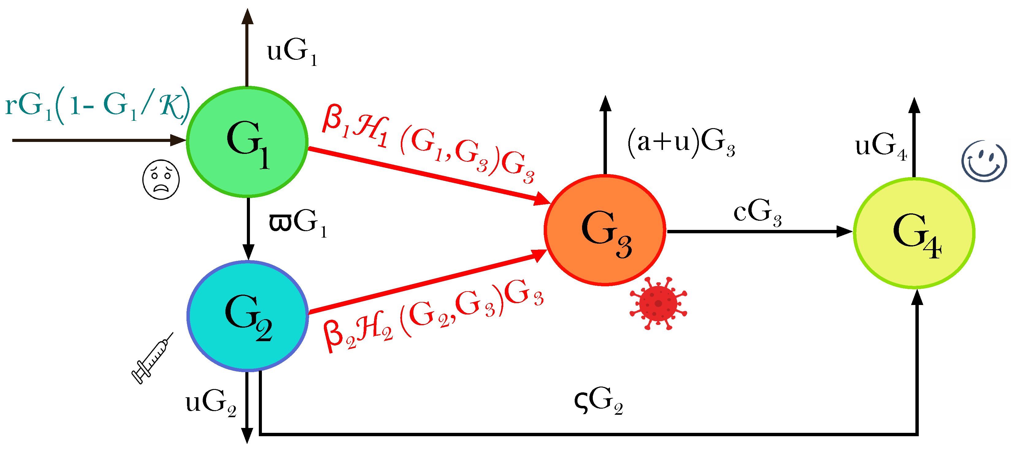
| Group | Biological Classification |
|---|---|
| Sensitive people | |
| Vaccinated people | |
| Infected people | |
| Recovered people with total immunity |
| Name | Expression |
|---|---|
| Bilinear | |
| Saturated 2 | , () |
| Dual saturated | , () |
| Beddington-DeAngelis | , () |
| Crowley-Martin | , () |
| Modified Crowley-Martin | , () |
| Name | Expression |
|---|---|
| Bilinear | |
| Saturated | , () |
| Dual saturated | , () |
| Beddington-DeAngelis | , () |
| Crowley-Martin | , () |
| Modified Crowley-Martin | , () |
| Stochastic Parameters | Values |
|---|---|
| (0.051, 0.042, 0.07, 0.0315) | |
| (0.001, 0.002, 0.004, 0.001) | |
| (0.01, 0.011, 0.0101, 0.01025) | |
| (0.0014, 0.0012, 0.0071, 0.0011) |
| Stochastic Parameters | Values |
|---|---|
| (0.11, 0.104, 0.12, 0.08) | |
| (0.01, 0.01, 0.01, 0.01) | |
| (0.1, 0.1, 0.201, 0.125) | |
| (0.01, 0.01, 0.01, 0.01) |
Disclaimer/Publisher’s Note: The statements, opinions and data contained in all publications are solely those of the individual author(s) and contributor(s) and not of MDPI and/or the editor(s). MDPI and/or the editor(s) disclaim responsibility for any injury to people or property resulting from any ideas, methods, instructions or products referred to in the content. |
© 2023 by the authors. Licensee MDPI, Basel, Switzerland. This article is an open access article distributed under the terms and conditions of the Creative Commons Attribution (CC BY) license (https://creativecommons.org/licenses/by/4.0/).
Share and Cite
Sabbar, Y.; Khan, A.; Din, A.; Tilioua, M. New Method to Investigate the Impact of Independent Quadratic α-Stable Poisson Jumps on the Dynamics of a Disease under Vaccination Strategy. Fractal Fract. 2023, 7, 226. https://doi.org/10.3390/fractalfract7030226
Sabbar Y, Khan A, Din A, Tilioua M. New Method to Investigate the Impact of Independent Quadratic α-Stable Poisson Jumps on the Dynamics of a Disease under Vaccination Strategy. Fractal and Fractional. 2023; 7(3):226. https://doi.org/10.3390/fractalfract7030226
Chicago/Turabian StyleSabbar, Yassine, Asad Khan, Anwarud Din, and Mouhcine Tilioua. 2023. "New Method to Investigate the Impact of Independent Quadratic α-Stable Poisson Jumps on the Dynamics of a Disease under Vaccination Strategy" Fractal and Fractional 7, no. 3: 226. https://doi.org/10.3390/fractalfract7030226
APA StyleSabbar, Y., Khan, A., Din, A., & Tilioua, M. (2023). New Method to Investigate the Impact of Independent Quadratic α-Stable Poisson Jumps on the Dynamics of a Disease under Vaccination Strategy. Fractal and Fractional, 7(3), 226. https://doi.org/10.3390/fractalfract7030226