Dynamics and Stability of a Fractional-Order Tumor–Immune Interaction Model with B-D Functional Response and Immunotherapy

Abstract

In this paper, we investigate a fractional-order tumor–immune interaction model with B-D function item and immunotherapy. First, the existence, uniqueness and nonnegativity of the solutions of the model are established. Second, the local and global asymptotic stability of some tumor-free equilibrium points and a unique positive equilibrium point are obtained. Finally, we use numerical simulation method to visualize and verify the theoretical conclusions. It is known that the fractional-order parameter $\beta$ has a stabilization effect, and the tumor cells can be destroyed or controlled by using immunotherapy.

1. Introduction

In this paper, we mainly investigated a fractional-order tumor–immune interaction model with B-D function item and immunotherapy as follows

$$\{\begin{array}{l}{}_0{}^{c}D{}_t^{\beta }u(t)=av-m_{1}u+\frac{k_{1}uw}{1+w}+s_1,\\ {}_0{}^{c}D{}_t^{\beta }v(t)=v\left(b-v\right)-\frac{cuv}{u+v+d},\\ {}_0{}^{c}D{}_t^{\beta }w(t)=\frac{k_{2}uv}{u+v+d}-m_{2}w+s_2,\\ u\left(0\right)=u_0\ge 0,v\left(0\right)=v_0\ge 0,w\left(0\right)=w_0\ge 0,\end{array}$$

(1)

where $u(t)$ stand for the density of effector cells that are cytotoxic to the tumor cells; $v(t)$ represents the density of tumor cells; $w(t)$ is the concentration of interleukin-2 (IL-2); $a$ is the antigenicity of the tumor; $b$ is the environmental carrying capacity; $k_1,c,k_2$ are the uptake velocity when all sites are saturated by the substrate; $1/m_1$ is the natural average lifespan; $m_2$ is the loss or degraded rate of IL-2; $d$ is the half saturation constant; $s_1$ represents the treatment by an external source of effector cells (ACI); $s_2$ represents the treatment by an external input of IL-2 into the model, ${}_0{}^{c}D{}_t^{\beta }$ is the standard Caputo differentiation; and $uv/\left(u+v+d\right)$ is the Beddington–DeAngelis (denoted by B-D) functional response.

A tumor is a new organism formed by local tissue cell proliferation under the action of various tumorigenic factors. Tumors can also be classified as benign, precancerous, or malignant, with malignant tumors also known as cancers. Because cancer cells divide uncontrollably and can invade other tissues, the individual fatality rate for cancer is extremely high. The safe treatment of cancer is an important issue being studied in the medical model at present. Numerous studies have shown that host immune cells have an inhibitory effect on tumor growth [1,2,3,4,5,6,7].

Immunotherapy is a cancer treatment that utilizes cytokines and adoptive cell immunotherapy (ACI). Moreover, interleukin-2 (IL-2), the major cytokine responsible for lymphocyte activation, growth, and differentiation, is mainly produced by CD4⁺ T cells. The injection of cultured immune cells with antitumor reactivity into a tumor-carrying host is performed by ACI, using either lymphokine-activated killer (LAK) therapy or tumor-infiltrating lymphocyte (TIL) therapy in combination with abundant IL-2. By applying LAK therapy or TIL therapy or by applying both therapies simultaneously, Krischner et al. [8] researched a model describing tumor–immune dynamics together with the feature of IL-2 dynamics. In [9], we have proposed a fractional-order model with a Holling II function item describing the interaction between effector cells, tumor cells, and IL-2 as follows

$$\{\begin{array}{l}{}_0{}^{c}D{}_t^{\beta }u(t)=av-m_{1}u+\frac{k_{1}uw}{1+w}+s_1,\\ {}_0{}^{c}D{}_t^{\beta }v(t)=v\left(1-bv\right)-\frac{cuv}{v+d},\\ {}_0{}^{c}D{}_t^{\beta }w(t)=\frac{k_{2}uv}{1+v}-m_{2}w+s_2,\\ u\left(0\right)=u_0\ge 0,v\left(0\right)=v_0\ge 0,w\left(0\right)=w_0\ge 0,\end{array}$$

(2)

where ${}_0{}^{c}D{}_t^{\beta }$ is the standard Caputo differentiation and $\beta \in \left(0,1\right)$, the Caputo fractional derivative of order $\beta$, is defined as [10,11]

$${}_0{}^{c}D{}_t^{\beta }h(x)=\frac{1}{\Gamma (m-\beta )}{\displaystyle {\int }_{t_0}^t{(x-t)}^{m-\beta -1}{h}^{(m)}(t)dt,m-1<\beta <m,m\in \mathbb{N}.}$$

Fractional-order differential equations present an outstanding description of certain nonlinear practical problems. Many real biological models have memory, and fractional models may be better suited to describing the real situation than integer models, which have the advantage that they describe the entire time domain of a physical process, whereas integer models relate to the local properties of a location. So, we have studied the asymptotic behavior analysis of a fractional-order tumor–immune interaction model with Holling functional response function and immunotherapy in [9].

However, functional responses are of important biological significance in the model (Equation (2)), which represents the average conversion rate among three types of cells. It is easy to see that the above Holling II reaction functions in (Equation (2)) are only dependent on the transformed cells and are not affected by the number of the newborn cells. In order to formulate mutual interference among cells, Beddington [12] and DeAngelis [13] established so-called Beddington–DeAngelis (denoted by B-D) functional response given by $\frac{uv}{u+v+d}$. Therefore, by introducing the B-D functional response into the model (Equation (2)) and taking into account the fractional-order equation and the important influence of effector cells on the immunotherapy process, we established model (Equation (1)), which can more accurately simulate the transformation relations and laws between effector cells, tumor cells, and IL-2, and enrich the research results of fractional biological mathematical ODE models.

This paper is organized as follows. In Section 2, we state our main results about the existence, uniqueness, and nonnegativity of the solutions of the model (Equation (1)) by using the standard comparison theorem and the local Lipschitz condition. Meanwhile, there are some equilibrium points, depending on what treatment is not used and whether the tumor is curable. Additionally, sufficient conditions on the local and global asymptotic stability of these equilibrium points are proved using the linearization method and the Routh–Hurwitz conditions in Section 3, for the cases of the realistic tumor-free equilibriums and the unique interior equilibriums, respectively. Finally, some numerical simulations are given to illustrate and visualize our theoretical results in Section 4.

2. Uniqueness and Nonnegativity of Solutions

In this section, we study the existence, uniqueness, and nonnegativity of the solutions of the model (Equation (1)). Then, we need the following lemma to prove the existence and uniqueness of the solutions of the fractional-order model (Equation (1)).

Lemma 1

(see [14,15]). Consider the model with initial condition $h(t_0)$

$${}_{t_0}{}^{c}D{}_t^{\beta }h(t)=h\left(t,x\right),$$

(3)

where $\beta \in \left(0,1\right)$ and $h:\left[t_0,\infty \right)\times \mathsf{\Omega }\to {ℝ}^N$, $\mathsf{\Omega }\in {ℝ}^N$, if $h\left(t,x\right)$ meets the local Lipschitz condition depending on $x$, then the model presents a unique solution of Equation (3).

Theorem 1.

Define $\mathsf{\Omega }=\left\{\left(u,v,w\right)\in {ℝ}^3:\max \left\{\left|u\right|,\left|v\right|,\left|w\right|\right\}\le \tilde{M}\right\}$. For every initial condition$X_0=$ $\left(u_0,v_0,w_0\right)\in \mathsf{\Omega }$, the model (Equation (1)) has a unique solution for all $t\ge 0$.

Proof. 

Set $T\in \left(0,+\infty \right)$; we denote $X={\left(u,v,w\right)}^T$ and $\tilde{X}={\left(\tilde{u},\tilde{v},\tilde{w}\right)}^T$ in the region $\mathsf{\Omega }\times \left(0,T\right]$. Consider a mapping defined by $H(X)={\left(H_1(X),H_2(X),H_3(X)\right)}^T$, where

$$\begin{array}{l}{H}_1(X)=av-m_{1}u+\frac{k_{1}uw}{1+w}+s_1,\\ H_2(X)=v\left(b-v\right)-\frac{cuv}{u+v+d},\\ H_3(X)=\frac{k_{2}uv}{u+v+d}-m_{2}w+s_2.\end{array}$$

(4)

For any $X,\tilde{X}\in \mathsf{\Omega }$, according to (Equation (4)), we obtain the following inequality

$$\begin{array}{l}\Vert H(X)-H(\tilde{X})\Vert \\ =\left|H_1(X)-H_1(\tilde{X})\right|+\left|H_2(X)-H_2(\tilde{X})\right|+\left|H_3(X)-H_3(\tilde{X})\right|\\ =\left|av-m_{1}u+\frac{k_{1}uw}{1+w}+s_1-a\tilde{v}+m_1\tilde{u}-\frac{k_1\tilde{u}\tilde{w}}{1+\tilde{w}}-s_1\right|+\left|v\left(b-v\right)-\frac{cuv}{u+v+d}-\tilde{v}\left(b-\tilde{v}\right)+\frac{c\tilde{u}\tilde{v}}{\tilde{u}+\tilde{v}+d}\right|\\ +\left|\frac{k_{2}uv}{u+v+d}-m_{2}w+s_2-\frac{k_2\tilde{u}\tilde{v}}{\tilde{u}+\tilde{v}+d}+m_2\tilde{w}-s_2\right|\\ =\left|a\left(v-\tilde{v}\right)+\left(\frac{k_1\tilde{w}}{1+\tilde{w}}-m_1\right)\left(u-\tilde{u}\right)+\frac{k_1\tilde{u}\left(w-\tilde{w}\right)}{\left(1+w\right)\left(1+\tilde{w}\right)}\right|\\ +|\left[b-\left(v+\tilde{v}\right)-\frac{cu}{u+v+d}+\frac{cu\tilde{v}}{\left(u+v+d\right)\left(\tilde{u}+\tilde{v}+d\right)}\right]\left(v-\tilde{v}\right)-\frac{c\tilde{v}\left(v+d\right)}{\left(u+v+d\right)\left(\tilde{u}+\tilde{v}+d\right)}\left(u-\tilde{u}\right)|\\ +\left|\frac{k_2\tilde{u}\left(u+d\right)}{\left(u+v+d\right)\left(\tilde{u}+\tilde{v}+d\right)}\left(v-\tilde{v}\right)+\left[\frac{k_{2}v}{u+v+d}-\frac{k_2\tilde{u}v}{\left(u+v+d\right)\left(\tilde{u}+\tilde{v}+d\right)}\right]\left(u-\tilde{u}\right)-m_2\left(w-\tilde{w}\right)\right|\\ \le a\left|v-\tilde{v}\right|+\left(k_1+m_1\right)\left|u-\tilde{u}\right|+k_1\tilde{M}\left|w-\tilde{w}\right|+2k_2\left|u-\tilde{u}\right|+k_2\left|v-\tilde{v}\right|+m_2\left|w-\tilde{w}\right|+\\ \left(b+2c+2\tilde{M}\right)\left|v-\tilde{v}\right|+c\left|u-\tilde{u}\right|\\ =\left(k_1+m_1+2k_2+c\right)\left|u-\tilde{u}\right|+\left(a+k_2+b+2c+2\tilde{M}\right)\left|v-\tilde{v}\right|+\left(k_1\tilde{M}+m_2\right)\left|w-\tilde{w}\right|\\ \le L\Vert X-\tilde{X}\Vert ,\end{array}$$

where $L=\max \left\{k_1+m_1+2k_2+c,a+k_2+b+2c+2\tilde{M},k_1\tilde{M}+m_2\right\}$; then $H(X)$ with respect to $X$ satisfies the local Lipschitz condition, and model (Equation (3)) has a unique solution.

Thanks to the above analysis, in the following, we establish the conditions for the nonnegativity of the solutions of the model (Equation (1)). □

Theorem 2.

We denote ${ℝ}^{*}=\left\{x\in ℝ:x\ge 0\right\}$ and ${\mathsf{\Omega }}^{*}=\left\{\left(u,v,w\right)\in \mathsf{\Omega }:u,vandw\in {ℝ}^{*}\right\}$. For every initial condition $X_0=\left(u_0,v_0,w_0\right)\in {ℝ}_{+}^3$, all solutions of model (Equation (1)) are nonnegative.

Proof. 

To end this Theorem, we will adopt the method of contradiction proof. Assume that there exists $\underset{˜}{t}\in \left[0,+\infty \right)$ such that the solutions of model (Equation (1)) pass through the $u$, $v$, or $w$ axes. Set $\beta$ to be defined in (Equation (3)); the results can be divided into the following three cases:

(i)

If $u\left(\underset{˜}{t}\right)>0$, $v\left(\underset{˜}{t}\right)>0$, and $w\left(\underset{˜}{t}\right)=0$, there is $\tilde{t}>\underset{˜}{t}$ and $0<\tilde{t}-\underset{˜}{t}\ll 1$. When $t\in \left[\underset{˜}{t},\tilde{t}\right)$, it is known that $u\left(t\right)>0$, $v\left(t\right)>0$ and $w\left(t\right)<0$. From the third equation of model (Equation (1)), we can derive ${}_0{}^{c}D{}_t^{\beta }w(t)>-m_{2}w$ and then $w(t)>w(0)E_{\beta }\left[\left(-m_2\right)t^{\beta }\right]$ with $t\in \left[\underset{˜}{t},\tilde{t}\right)$. The Mittag–Leffler function is $E_{\beta ,\gamma }(t)={\displaystyle {\sum }_{s=0}^{\infty }\left[t^s/\Gamma \left(s\beta +\gamma \right)\right]}$ and $E_{\beta }(t)=E_{\beta ,1}(t)$ with $\beta ,\gamma >0$ [16]. We know that the Mittag–Leffler function is positive in [11,14,15], then $E_{\beta }(t)>0$. By using the standard comparison theorem [9,17], we obtain $w(t)>0$ for all $t\in \left[\underset{˜}{t},\tilde{t}\right)$, and $\beta \in \left(0,1\right)$, which contradicts the hypothesis. The same can be said for the following two cases:

(ii)

Suppose that $u\left(\underset{˜}{t}\right)>0$, $w\left(\underset{˜}{t}\right)>0$ and $v\left(\underset{˜}{t}\right)=0$, there is $\tilde{t}>\underset{˜}{t}$ and $0<\tilde{t}-\underset{˜}{t}\ll 1$. When $t\in \left[\underset{˜}{t},\tilde{t}\right)$, it is known that $u\left(t\right)>0$, $w\left(t\right)>0$, and $v\left(t\right)<0$. From the second equation of the model (Equation (1)), we can derive ${}_0{}^{c}D{}_t^{\beta }v(t)>bv$ and then $v(t)>v(0)E_{\beta }\left(b{t}^{\beta }\right)$ with $t\in \left[\underset{˜}{t},\tilde{t}\right)$. Then, we obtain $v(t)>0$ for all $t\in \left[\underset{˜}{t},\tilde{t}\right)$, and $\beta \in \left(0,1\right)$, which contradicts the hypothesis.

(iii)

Suppose that $v\left(\underset{˜}{t}\right)>0$, $w\left(\underset{˜}{t}\right)>0$, and $u\left(\underset{˜}{t}\right)=0$, there is $\tilde{t}>\underset{˜}{t}$ and $0<\tilde{t}-\underset{˜}{t}\ll 1$. When $t\in$$\left[\underset{˜}{t},\tilde{t}\right)$, it is known that $v\left(t\right)>0$, $w\left(t\right)>0$, and $u\left(t\right)<0$. From the first equation of model (Equation (1)), we can derive ${}_0{}^{c}D{}_t^{\beta }u(t)>\left(k_1-m_1\right)u$ and then $u(t)>u(0)E_{\beta }\left[\left(k_1-m_1\right)t^{\beta }\right]$ with $t\in \left[\underset{˜}{t},\tilde{t}\right)$. Then, we obtain $u(t)>0$ for all $t\in \left[\underset{˜}{t},\tilde{t}\right)$, and $\beta \in \left(0,1\right)$, which contradicts the hypothesis. □

According to the above method, the nonnegativity of the other solutions can be proved, and the proof process is omitted here.

According to the above cases, it follows that the solutions of model (Equation (1)) are nonnegative.

3. Equilibria and Stability

In this section, all positive constant equilibrium points of model (Equation (1)) will be analyzed. From a direct calculation, we know that model (Equation (1)) has four nonnegative equilibrium points in order to simulate the disappearance of the tumor cells; all the points at least have one zero element.

(i)

$A_1=\left(0,0,0\right)$, if $s_1=0$ and $s_2=0$,

(ii)

$A_2=\left(\frac{s_1}{m_1},0,0\right)$, if $s_1>0$ and $s_2=0$, tumor treatment by an external source of effector cells,

(iii)

$A_3=\left(0,0,\frac{s_2}{m_2}\right)$, if $s_1=0$ and $s_2>0$,

(iv)

$A_4=\left(\frac{s_1\left(m_2+s_2\right)}{m_1{m}_2+s_2\left(m_1-k_1\right)},0,\frac{s_2}{m_2}\right)$, if $s_1>0$, $s_2>0$ and $m_1{m}_2>s_2\left(k_1-m_1\right)$, tumor treatment by an external source of effector cells with an external input of IL-2 into the model (Equation (1)).

The points (i) and (iii) are not in line with the scope of actual medical research, because effector cells do not disappear under any circumstances; thus, these two points will not be discussed in depth in this section. However, the cases (ii) and (iv) are tumor-free equilibrium points in reality, it remains that if the tumor is cured, we will study these two cases and provide sufficient conditions, which is necessary for asymptotic stability in cases (ii) and (iv). Then, we only give the conditions that make model (Equation (1)) describe a unique positive equilibrium point $\widehat{A}=\left(\widehat{u},\widehat{v},\widehat{w}\right)$ and omit calculation the procedure. We can easily obtain the following results from [5].

Lemma 2.

If one of the following inequalities is true, model (Equation (1)) has a unique positive equilibrium point $\widehat{A}$.

$$\begin{gathered} s_1>a\left(d-c\right),\left(c-b-d\right)s_1^2+\left(abc-acd-a{b}^2+a{d}^2\right)s_1<a^{2}bd\left(c-d\right), \\ \frac{\left(m_1-k_1\right)bd}{c-b+v}>s_1\mathrm{and}{m}_1\ne k_1. \end{gathered}$$

(5)

$$s_1>ad,c{s}_1^2+\left(abc+a{d}^2\right)s_1<a^{2}bd\left(c-d\right),\frac{m_{1}bd}{c-b}>s_1\left(1+s_2\right)\mathrm{and}{m}_1=k_1.$$

(6)

where $\widehat{A}=\left(\widehat{u},\widehat{v},\widehat{w}\right)$ is given as follows

$$\begin{gathered} \widehat{u}=\frac{-{\widehat{v}}^2+\left(b-s\right)\widehat{v}+bd}{c-b+\widehat{v}}, \\ \widehat{w}=\frac{m_1\widehat{u}-a\widehat{v}-s_1}{(k_1-m_1)\widehat{u}+a\widehat{v}+s_1}, \\ \widehat{w}=\frac{(s_2+k_2\widehat{v})\widehat{u}+(\widehat{v}+d)s_2}{\widehat{u}+\widehat{v}+d}. \end{gathered}$$

In the following lemma, we give the conditions for the asymptotic stability.

Lemma 3.

Let $J(X)$ be the Jacobian matrix of model (Equation (1)); we linearize model (Equation (1)) at point $X=\left(u,v,w\right)$ and obtain

$$J(X)=H_X(X)=\left(\begin{array}{ccc}-m_1+\frac{k_{1}w}{1+w}& a& \frac{k_{1}u}{{\left(1+w\right)}^2}\\ \frac{-cv\left(v+d\right)}{{\left(u+v+d\right)}^2}& b-2v-\frac{cu\left(u+d\right)}{{\left(u+v+d\right)}^2}& 0\\ \frac{k_{2}v\left(v+d\right)}{{\left(u+v+d\right)}^2}& \frac{k_{2}u\left(u+d\right)}{{\left(u+v+d\right)}^2}& -m_2\end{array}\right),$$

(7)

where  $H(X)$  is defined in Theorem 1, let${\lambda }_j\left(j=1,2,\dots \right)$ be the eigenvalues of $J(X)$. If all eigenvalues ${\lambda }_j\left(j=1,2,\dots \right)$ satisfy $\left|\arg \left({\lambda }_i\right)\right|>\frac{\beta \pi }{2}$, equilibrium point $X$ is a local asymptotic stability; if some eigenvalues ${\lambda }_j\left(j=1,2,\dots \right)$ satisfy $\left|\arg \left({\lambda }_i\right)\right|>\frac{\beta \pi }{2}$ and others satisfy $\left|\arg \left({\lambda }_i\right)\right|<\frac{\beta \pi }{2}$, $X$  is a saddle point and unstable.

In the following, we give some conditions to prove the local asymptotic stability of $A_2$ and $A_4$ defined by Lemma 3.

Theorem 3.

Let $b,c$, $d$, $m_1$, and $s_1$ be defined in model (Equation (1)); we obtain the following statements

(i) 

If$\left(c-b\right)s_1>m_{1}bd$, then equilibrium point$A_2$is a local asymptotic stability.

(ii) 

If$\left(c-b\right)s_1<m_{1}bd$, then equilibrium point$A_2$is a saddle point and unstable.

Proof. 

Substituting $X=A_2$ into (Equation (7)), we have

$$J(A_2)=\left(\begin{array}{ccc}-m_1& a& \frac{k_1{s}_1}{m_1}\\ 0& b-\frac{c{s}_1}{s_1+m_{1}d}& 0\\ 0& \frac{k_2{s}_1}{s_1+m_{1}d}& -m_2\end{array}\right),$$

it is easy to see that the eigenvalues of $J(A_2)$ are

$$\begin{array}{l}{\lambda }_1=-m_1,\\ {\lambda }_2=-m_2,\\ {\lambda }_3=b-\frac{c{s}_1}{s_1+m_{1}d},\end{array}$$

if $\left(c-b\right)s_1>m_{1}bd$, that is $\arg \left({\lambda }_3\right)=\pi$, then all the other ${\lambda }_i\left(i=1,2,3\right)$ will also satisfy $\arg \left({\lambda }_1\right)$$=\arg \left({\lambda }_2\right)=\arg \left({\lambda }_3\right)=\pi$. Therefore, $\left|\arg \left({\lambda }_i\right)\right|>\frac{\beta \pi }{2}(i=1,2,3)$ for $\beta \in \left(0,1\right)$. It follows from Lemma 2 that the equilibrium point $A_2$ is a local asymptotic stability. However, if $\left(c-b\right)s_1<m_{1}bd,$$\arg \left({\lambda }_1\right)=\arg \left({\lambda }_2\right)=\pi$ and $\arg \left({\lambda }_3\right)=0$, based on Lemma 2, $\left|\arg \left({\lambda }_i\right)\right|<\frac{\beta \pi }{2}(i=1,2,3)$ for $\beta \in$$\left(0,1\right)$. Then, the equilibrium point $A_2$ is a saddle point and unstable. □

Theorem 4.

Let $b,c$, $d$, $m_1,m_2,s_1$, and$s_2$ be defined in model (Equation (1)); we obtain the following statements

(i)

If$s_2<m_1\left(m_2+s_2\right)$and$m_1{m}_{2}bd+s_{2}bd\left(m_1-k_1\right)<\left(c{s}_1-b{s}_1\right)\left(m_2+s_2\right)$, then equilibrium$A_4$is a local asymptotic stability.

(ii)

If$s_2>m_1\left(m_2+s_2\right)$or$m_1{m}_{2}bd+s_{2}bd\left(m_1-k_1\right)>\left(c{s}_1-b{s}_1\right)\left(m_2+s_2\right)$, then equilibrium$A_2$is a saddle point and unstable.

Proof. 

Substituting $X=A_4$ into (Equation (7)), we obtain

$$J(A_4)=\left(\begin{array}{ccc}-m_1+\frac{s_2}{m_2+s_2}& a& \Upsilon \\ 0& b-\frac{c{s}_1\left(m_2+s_2\right)}{s_1\left(m_2+s_2\right)+m_1{m}_{2}d+s_{2}d\left(m_1-k_1\right)}& 0\\ 0& \frac{k_2{s}_1\left(m_2+s_2\right)}{s_1\left(m_2+s_2\right)+m_1{m}_{2}d+s_{2}d\left(m_1-k_1\right)}& -m_2\end{array}\right),$$

where $\Upsilon =\frac{m_2}{m_2+s_2}\cdot \frac{k_1{s}_1}{m_1{m}_2+\left(m_1-k_1\right)s_2}$ and it is clear that the eigenvalues of $J(A_4)$ are

${\lambda }_1=-m_2$,

${\lambda }_2=-m_1+\frac{s_2}{m_2+s_2}$,

${\lambda }_3=b-\frac{c{s}_1\left(m_2+s_2\right)}{s_1\left(m_2+s_2\right)+m_1{m}_{2}d+s_{2}d\left(m_1-k_1\right)}.$

If $s_2<m_1\left(m_2+s_2\right)$ and $m_1{m}_{2}bd+s_{2}bd\left(m_1-k_1\right)<\left(c{s}_1-b{s}_1\right)\left(m_2+s_2\right)$, that is $\arg \left({\lambda }_2\right)=\arg \left({\lambda }_3\right)$$=\pi$, then all the other ${\lambda }_i\left(i=1,2,3\right)$ will also satisfy $\arg \left({\lambda }_1\right)=\arg \left({\lambda }_2\right)=\arg \left({\lambda }_3\right)=\pi$. Therefore, from Lemma 2, we obtain $\left|\arg \left({\lambda }_i\right)\right|>$ $\frac{\beta \pi }{2}(i=1,2,3)$ for $\beta \in \left(0,1\right)$, the equilibrium $A_4$ is a local asymptotic stability. However, if $s_2>m_1\left(m_2+s_2\right)$, $\arg \left({\lambda }_2\right)=0$. Additionally, if $m_1{m}_{2}bd+s_{2}bd\left(m_1-k_1\right)>$$\left(c{s}_1-b{s}_1\right)\left(m_2+s_2\right)$, $\arg \left({\lambda }_3\right)=0$, then the equilibrium point $A_4$ is a saddle point and unstable. □

In the following, applying the Hurwitz conditions, we roughly provide the local asymptotically stability of the unique positive equilibrium point $\widehat{A}$.

Theorem 5.

Let $B(q)$ and $q_3$ be defined in (Equations (8) and (9)); if $m_1-k_1-b+m_2>0$, $q_3>0$ and $B(q)$$>0$, then $\widehat{A}$ is locally asymptotically stable.

Proof. 

Substituting $X=\widehat{A}$ into (Equation (7)), we have

$$J(\widehat{A})=\left(\begin{array}{ccc}-m_1+\frac{k_1\widehat{w}}{1+\widehat{w}}& a& \frac{k_1\widehat{u}}{{\left(1+\widehat{w}\right)}^2}\\ \frac{-c\widehat{v}\left(\widehat{v}+d\right)}{{\left(\widehat{u}+\widehat{v}+d\right)}^2}& b-2\widehat{v}-\frac{c\widehat{u}\left(\widehat{u}+d\right)}{{\left(\widehat{u}+\widehat{v}+d\right)}^2}& 0\\ \frac{k_2\widehat{v}\left(\widehat{v}+d\right)}{{\left(\widehat{u}+\widehat{v}+d\right)}^2}& \frac{k_2\widehat{u}\left(\widehat{u}+d\right)}{{\left(\widehat{u}+\widehat{v}+d\right)}^2}& -m_2\end{array}\right),$$

treating $J(\widehat{A})$ as the roots of $K(\lambda )={\lambda }^3+q_1{\lambda }^2+q_2\lambda +q_3=0$, then we can obtain the following equations

$$\begin{array}{l}{q}_1=m_1-\frac{k_1\widehat{w}}{1+\widehat{w}}-b+2\widehat{v}+\frac{c\widehat{u}\left(\widehat{u}+d\right)}{{\left(\widehat{u}+\widehat{v}+d\right)}^2}+m_2,\\ q_2=\left(\frac{k_1\widehat{w}}{1+\widehat{w}}-m_1\right)\left[b-2\widehat{v}-m_2-\frac{c\widehat{u}\left(\widehat{u}+d\right)}{{\left(\widehat{u}+\widehat{v}+d\right)}^2}\right]-m_2\left[b-2\widehat{v}-\frac{c\widehat{u}\left(\widehat{u}+d\right)}{{\left(\widehat{u}+\widehat{v}+d\right)}^2}\right]\\ +\frac{ac\widehat{v}\left(\widehat{v}+d\right)}{{\left(\widehat{u}+\widehat{v}+d\right)}^2}-\frac{k_1\widehat{u}}{{\left(1+\widehat{w}\right)}^2}\cdot \frac{k_2\widehat{v}\left(\widehat{v}+d\right)}{{\left(\widehat{u}+\widehat{v}+d\right)}^2},\\ q_3=\left[b-2\widehat{v}-\frac{c\widehat{u}\left(\widehat{u}+d\right)}{{\left(\widehat{u}+\widehat{v}+d\right)}^2}\right]\left[\frac{k_1\widehat{u}}{{\left(1+\widehat{w}\right)}^2}\cdot \frac{k_2\widehat{v}\left(\widehat{v}+d\right)}{{\left(\widehat{u}+\widehat{v}+d\right)}^2}-m_1{m}_2+\frac{k_1{m}_2\widehat{w}}{1+\widehat{w}}\right]\\ +\frac{c\widehat{v}\left(\widehat{v}+d\right)}{{\left(\widehat{u}+\widehat{v}+d\right)}^2}\cdot \frac{k_2\widehat{u}\left(\widehat{u}+d\right)}{{\left(\widehat{u}+\widehat{v}+d\right)}^2}\cdot \frac{k_1\widehat{u}}{{\left(1+\widehat{w}\right)}^2}+\frac{ac{m}_2\widehat{v}\left(\widehat{v}+d\right)}{{\left(\widehat{u}+\widehat{v}+d\right)}^2},\end{array}$$

(8)

if

$$\begin{gathered} q_1=m_1-\frac{k_1\widehat{w}}{1+\widehat{w}}-b+2\widehat{v}+\frac{c\widehat{u}\left(\widehat{u}+d\right)}{{\left(\widehat{u}+\widehat{v}+d\right)}^2}+m_2>m_1-k_1-b+m_2>0, \\ {q}_3>0, \end{gathered}$$

$$B(q)=q_1{q}_2-q_3>0$$

(9)

according to the Hurwitz conditions [18], all eigenvalues of $J(\widehat{A})$ have negative real parts, we obtain the local stability conditions of $\widehat{A}$. □

Next, we present the conditions for the global stability of $\widehat{A}$.

Theorem 6.

Suppose that $m_1>k_1$. Then, the nonnegative solution$\left(u,v,w\right)$to (Equation (1)) satisfies

$$\begin{array}{c}\underset{t\to \infty }{\lim }\underset{\mathsf{\Omega }}{\sup }u\left(x,t\right)\le \frac{ab+s_1}{m_1-k_1},\\ \underset{t\to \infty }{\lim }\underset{\mathsf{\Omega }}{\sup }v\left(x,t\right)\le b,\\ \underset{t\to \infty }{\lim }\underset{\mathsf{\Omega }}{\sup }w\left(x,t\right)\le \frac{1}{m_2}\left(k_2\cdot \frac{ab+s_1}{m_1-k_1}+s_2\right).\end{array}$$

Proof. 

To end this Theorem, we will adopt the method of the comparison principle [17]. From the second equation of the model (Equation (1)), we can verify that the sufficient conditions $v\left(b-v\right)-\frac{cuv}{u+v+d}$$\le v\left(b-v\right)$. Then, there exists some $t_1\in \left(0,\infty \right)$ such that $v\left(x,t\right)\le b+{\epsilon }_1$ for any positive constant ${\epsilon }_1$. Notice with this result, we obtain that $av-m_{1}u+\frac{k_{1}uw}{1+w}+s_1\le s_1-\left(m_1-k_1\right)u$$+ab$ with $\left[t_1,\infty \right)$$\times \mathsf{\Omega }$; thus, there exists $t_2\in \left[t_1,\infty \right)$ such that $u\left(x,t\right)\le \frac{ab+s_1}{m_1-k_1}+{\epsilon }_2$ for any nonnegative ${\epsilon }_2$. Finally, we obtain directly that there exists some $t_3\in \left[t_2,\infty \right)$ such that $\beta \in \frac{1}{m_2}\left(k_2\cdot \frac{ab+s_1}{m_1-k_1}+s_2\right)$$+{\epsilon }_3$ for any constant ${\epsilon }_3$ on $\left[t_2,\infty \right)\times \mathsf{\Omega }$. Therefore, by the arbitrariness of ${\epsilon }_1$, ${\epsilon }_2$, and ${\epsilon }_3$, the desired result has been obtained. □

Next, we use the Lyapunov function method to study the global stability of the unique positive equilibrium point $\widehat{A}$. We first define the following Lyapunov function

$$S(t)\triangleq S\left(u(t),v(t),w(t)\right)=\frac{1}{2}{\left(u-\widehat{u}\right)}^2+\left(v-\widehat{v}-\widehat{v}\ln \frac{v}{\widehat{v}}\right)+\frac{1}{2}{\left(w-\widehat{w}\right)}^2,$$

(10)

thanks to the famous Lyapunov stability; if ${}_0{}^{c}D{}_t^{\beta }S\left(t\right)\le 0$, the unique positive equilibrium $\widehat{A}$ is global stability.

Lemma 4

(see [19]). Set $x(t)\in {ℝ}^{*}$ and $\beta \in \left(0,1\right)$, we obtain the following inequality and $t>t_0$.

$${}_0{}^{c}D{}_t^{\beta }\left[x(t)-\widehat{x}-\widehat{x}\ln \frac{x(t)}{\widehat{x}}\right]\le \left[1-\frac{\widehat{x}}{x(t)}\right]{}_0{}^{c}D{}_t^{\beta }x(t),\widehat{x}\in {ℝ}^{*}.$$

Lemma 5

(see [20]). Let $x(t)\in {ℝ}^{*}$ be defined as a continuous and derivable function. Then, we obtain the following inequality and $t>t_0$

$$\frac{1}{2}{}_0{}^{c}D{}_t^{\beta }{x}^2(t)\le x(t){}_0{}^{c}D{}_t^{\beta }x(t).$$

Theorem 7.

Assume that (Equation (5)) holds. Then, the positive constant solution $\widehat{A}$ to (Equation (1)) is globally asymptotically stable if

$$\{\begin{array}{l}-m_1+k_1+\frac{a}{2}+\frac{c}{d}+k_2+\frac{k_1}{2}\cdot \frac{ab+s_1}{m_1-k_1}<0,\\ \frac{2c}{d}-1+\frac{a}{2}+\frac{k_2}{2}<0,\\ -m_2+\frac{3}{2}{k}_2+\frac{k_1}{2}\cdot \frac{ab+s_1}{m_1-k_1}<0\end{array}$$

.

Proof. 

To end this Theorem, we will use the model (Equation (1)) and integrate by parts, we have

$$\begin{array}{c}{}_0{}^{c}D{}_t^{\beta }S\left(t\right)\le \left(u-\widehat{u}\right){}_0{}^{c}D{}_t^{\beta }u(t)+\left[1-\frac{\widehat{v}}{v(t)}\right]{}_0{}^{c}D{}_t^{\beta }v(t)+\left(w-\widehat{w}\right){}_0{}^{c}D{}_t^{\beta }w(t)\\ =\left(u-\widehat{u}\right)\left(av-m_{1}u+\frac{k_{1}uw}{1+w}+s_1\right)+\left(v-\widehat{v}\right)\left(b-v-\frac{cu}{u+v+d}\right)\\ +\left(w-\widehat{w}\right)\left(\frac{k_{2}uv}{u+v+d}-m_{2}w+s_2\right).\end{array}$$

According to the definition of $\widehat{A}$, Lemma 4 and Lemma 5, we derive

$$\begin{array}{l}{}_0{}^{c}D{}_t^{\beta }S\left(t\right)\le \left(u-\widehat{u}\right){}_0{}^{c}D{}_t^{\beta }u(t)+\left[1-\frac{\widehat{v}}{v(t)}\right]{}_0{}^{c}D{}_t^{\beta }v(t)+\left(w-\widehat{w}\right){}_0{}^{c}D{}_t^{\beta }w(t)\\ =\left(u-\widehat{u}\right)\left(av-m_{1}u+\frac{k_{1}uw}{1+w}+s_1\right)+\left(v-\widehat{v}\right)\left(b-v-\frac{cu}{u+v+d}\right)\\ +\left(w-\widehat{w}\right)\left(\frac{k_{2}uv}{u+v+d}-m_{2}w+s_2\right)\\ ={\left(u-\widehat{u}\right)}^2\left(-m_1+\frac{k_{1}w}{1+w}\right)+{\left(v-\widehat{v}\right)}^2\left(\frac{c\widehat{u}}{\left(u+v+d\right)\left(\widehat{u}+\widehat{v}+d\right)}-1\right)\\ +\left(u-\widehat{u}\right)\left(v-\widehat{v}\right)\left(a+\frac{c\widehat{u}}{\left(u+v+d\right)\left(\widehat{u}+\widehat{v}+d\right)}-\frac{c}{u+v+d}\right)\\ +\frac{k_2\widehat{u}\left(u+d\right)\left(v-\widehat{v}\right)\left(w-\widehat{w}\right)}{\left(u+v+d\right)\left(\widehat{u}+\widehat{v}+d\right)}-m_2{\left(w-\widehat{w}\right)}^2\\ +\left(u-\widehat{u}\right)\left(w-\widehat{w}\right)\left(\frac{k_1\widehat{u}}{\left(1+w\right)\left(1+\widehat{w}\right)}+\frac{k_{2}v}{u+v+d}-\frac{k_2\widehat{u}v}{\left(u+v+d\right)\left(\widehat{u}+\widehat{v}+d\right)}\right)\\ \triangleq H(t),\end{array}$$

Thanks to Theorem 5, it is easy to see that $u\left(x,t\right)\le \frac{ab+s_1}{m_1-k_1},$ then

$$\begin{array}{l}H(t)\le {\left(u-\widehat{u}\right)}^2\left(-m_1+k_1\right)+\left(u-\widehat{u}\right)\left(v-\widehat{v}\right)\left(a+\frac{2c}{d}\right)+{\left(v-\widehat{v}\right)}^2\left(\frac{c}{d}-1\right)\\ +k_2\left(v-\widehat{v}\right)\left(w-\widehat{w}\right)-m_2{\left(w-\widehat{w}\right)}^2+\left(u-\widehat{u}\right)\left(w-\widehat{w}\right)\left(k_1\widehat{u}+2k_2\right)\\ \le {\left(u-\widehat{u}\right)}^2\left(-m_1+k_1+\frac{a}{2}+\frac{c}{d}+k_2+\frac{k_1}{2}\cdot \frac{ab+s_1}{m_1-k_1}\right)\\ +{\left(v-\widehat{v}\right)}^2\left(\frac{c}{d}-1+\frac{a}{2}+\frac{c}{d}+\frac{k_2}{2}\right)\\ +{\left(w-\widehat{w}\right)}^2\left(-m_2+\frac{3}{2}{k}_2+\frac{k_1}{2}\cdot \frac{ab+s_1}{m_1-k_1}\right).\end{array}$$

By direct scaling calculation, we easily prove that ${}_0{}^{c}D{}_t^{\beta }S\left(t\right)\le 0$ and the positive constant solution $\widehat{A}$ to (Equation (1)) is globally asymptotically stable if the following three conditions are satisfied

(i)

$-m_1+k_1+\frac{a}{2}+\frac{c}{d}+k_2+\frac{k_1}{2}\cdot \frac{ab+s_1}{m_1-k_1}<0,$

(ii)

$\frac{2c}{d}-1+\frac{a}{2}+\frac{k_2}{2}<0,$

(iii)

$-m_2+\frac{3}{2}{k}_2+\frac{k_1}{2}\cdot \frac{ab+s_1}{m_1-k_1}<0$.

So, we complete the proof of Theorem 7. □

4. Numerical Simulations

In this section, we will obtain some numerical simulations by using the fractional linear multistep methods and the predictor–corrector algorithm [21,22], which are applied to find the approximate solution of the fractional-order tumor–immune interaction model (Equation (1)). Therefore, we can visualize and verify the above theoretical conclusions. Note that from the above numerical simulation results, we easily obtain the following conclusions.

(i)

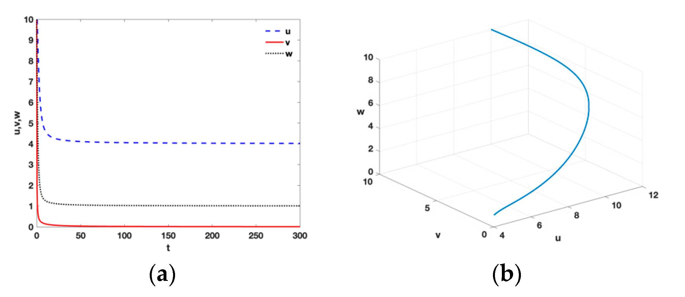
From Theorem 3, it follows that when $s_1=3$ and $s_2=0$, there is a realistic tumor-free equilibrium $A_2$$=(3,0,0)$ with $a=0.9$, $m_1=1$, $k_1=0.5$, $b=1$, $c=3$, $s_1=3$, $d=2.5$, $k_2=1$, $m_2=1$, $s_2=0$, and $\beta =0.9$. It can be observed in Figure 1 that the tumor-free equilibrium $A_2=(3,0,0)$ is locally asymptotically stable and it remains that the tumor is curable by using ACI therapy or ACI therapy and IL-2.

(ii)

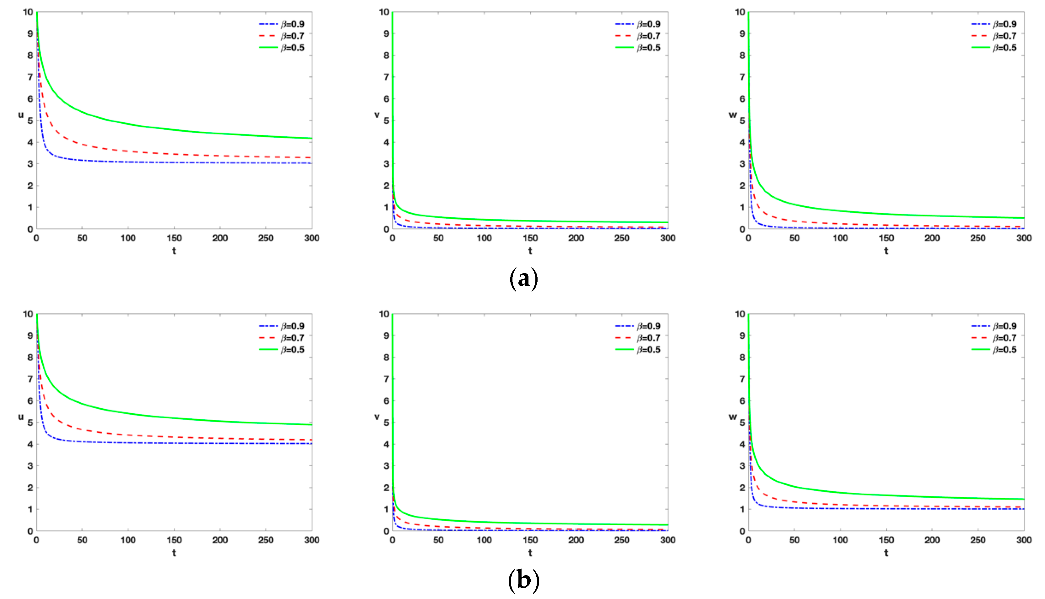
According to Theorem 4, we take $s_1=3$ and $s_2=1$, and there exists the tumor-free equilibrium $A_4$$=(4,0,1)$. See Figure 2; $A_4$ is locally asymptotically stable and remains that the tumor is curable by ACI therapy and the external input of IL-2 into the model (Equation (1)).

(iii)

From Figure 3, it is easy to see that as tumor cells $v$ of $A_2$ and $A_4$ are destroyed more quickly, the greater value of $\beta$. It is clearly known that the fractional-order parameter $\beta$ has a stabilization effect.

(iv)

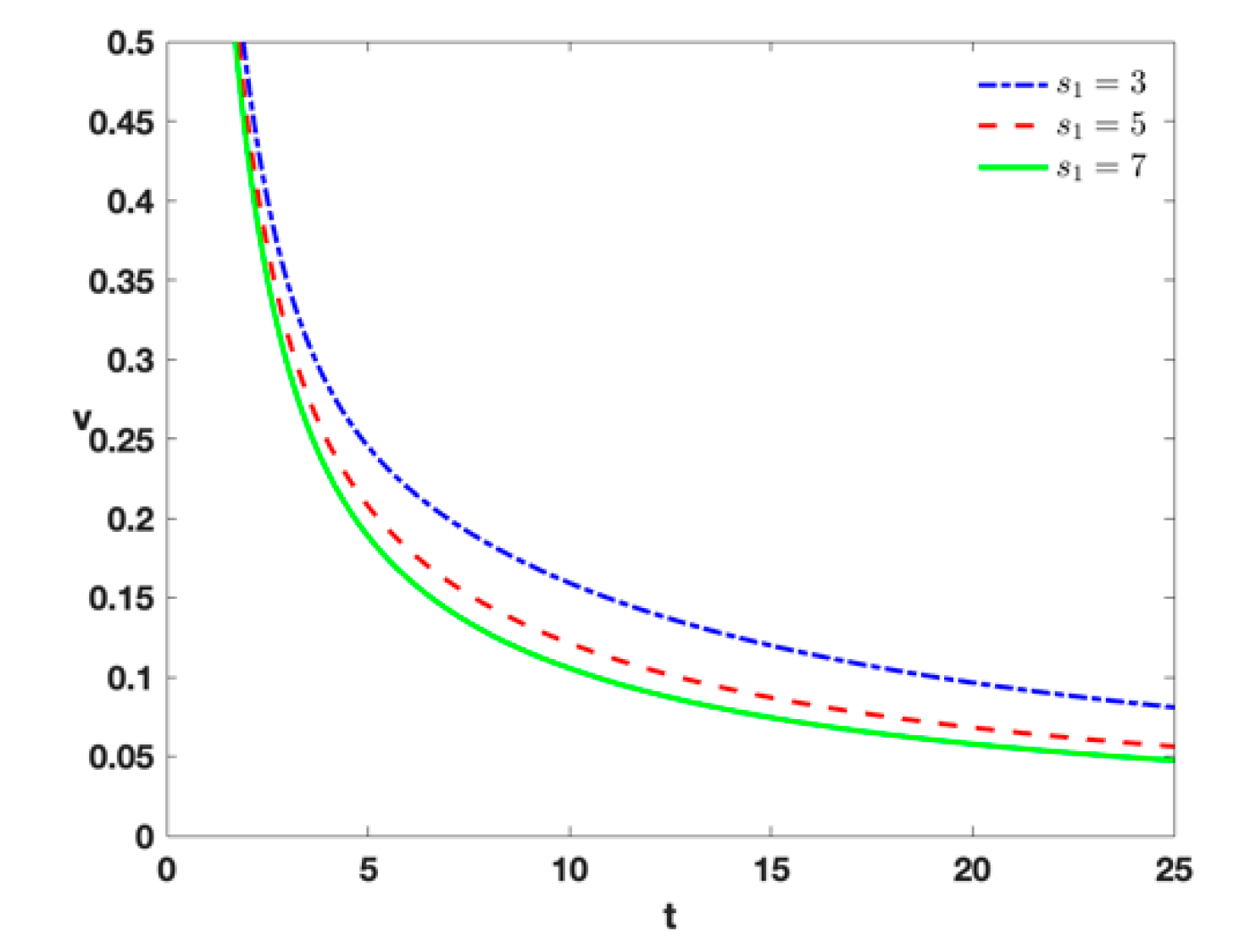
When $s_2=0$ and $s_1=3,5,7$, this refers to the injection of external effector cells to destroy the tumor cells. From Figure 4, it follows that as the speed of tumor elimination becomes larger, the value of $s_1$ becomes larger. However, as the number increases, the change becomes less and less obvious. Which means that there is also a critical value when the value $s_1$ is selected.

(v)

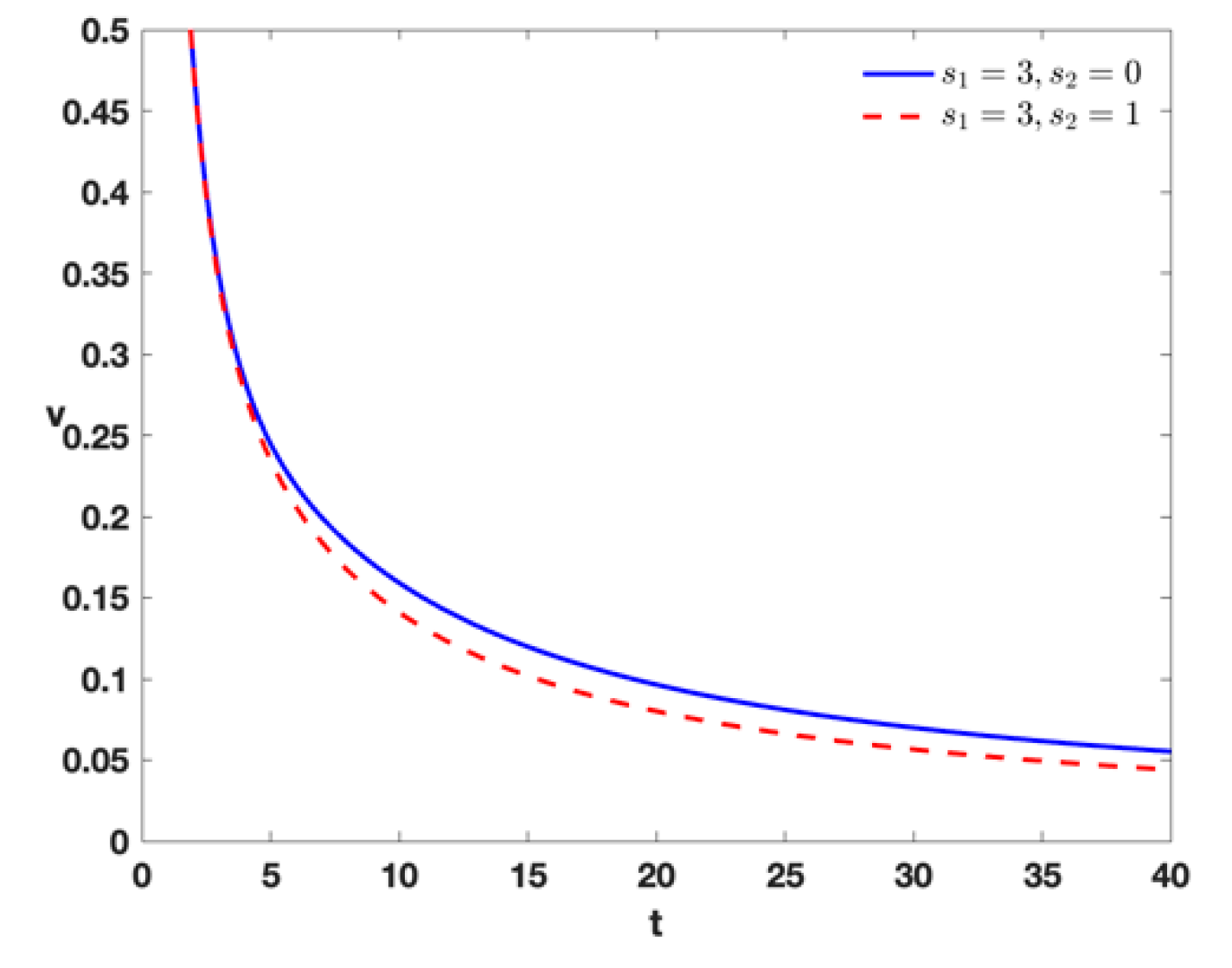
When $s_2=0$ and $s_1=3$, this indicates tumor therapy by external effector cells. When $s_2$$=1$ and $s_1=3$, this indicates tumor therapy by external effector cells and external input of IL-2 into the model (Equation (1)). This shows that the injection of external IL-2 enhanced the speed of tumor extinction in Figure 5.

(vi)

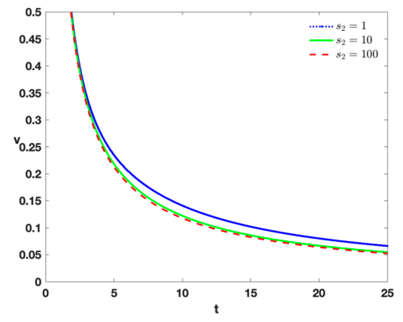
In order to investigate the impact of external input of IL-2 into the model (Equation (1)) with different positive values, Figure 6 indicates that with a larger value of $s_2$ and the same value of $s_1$, the speed of tumor extinction will be larger. Moreover, there is also a critical value when the value $s_2$ is selected.

(vii)

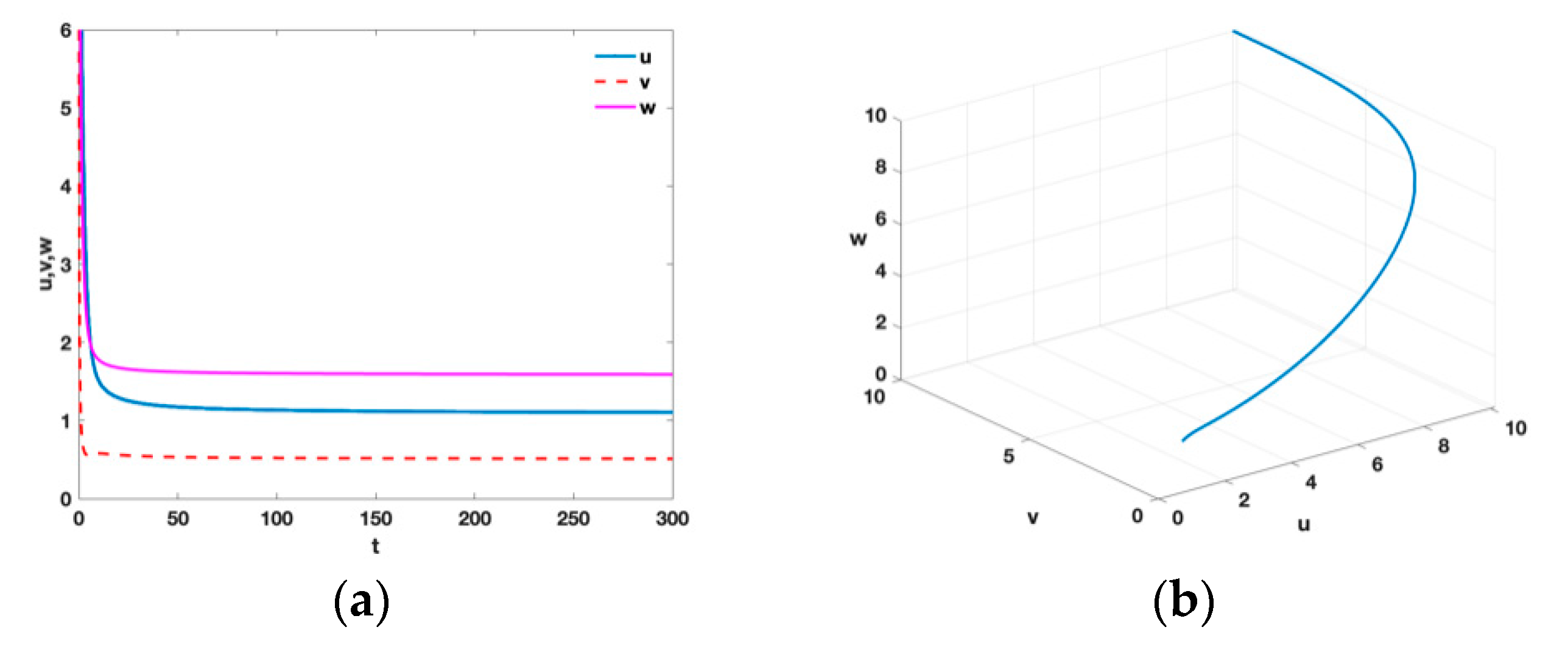
From Theorem 5, the tumor is incurable. However, immunotherapy can achieve an effective and stable tumor control. There is an equilibrium $\widehat{A}=\left(1.11,0.51,1.64\right)$ with $a=0.9$, $m_1$$=1$, $k_1=0.5$, $b=1$, $c=3$, $s_1=0.3$, $d=5$, $k_2=1$, $m_2=1$, $s_2=1.5$, and $\beta =0.9$. Figure 7 shows that the unique positive equilibrium $\widehat{A}$ is locally asymptotically stable.

(viii)

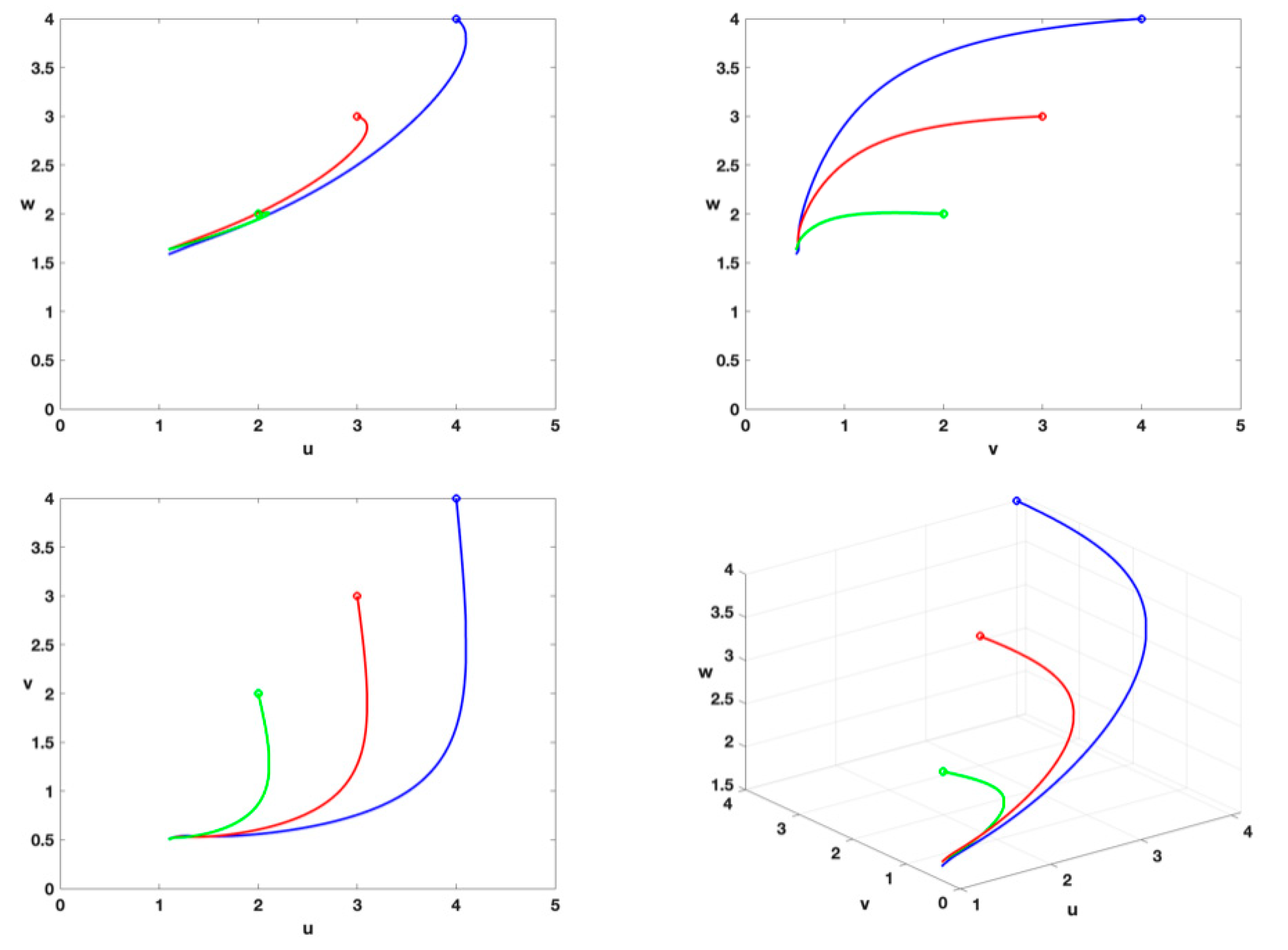
From Theorem 7, the tumor cells will be incurable. Figure 8 indicates that the unique positive equilibrium $\widehat{A}$ is always present and stable when the positive initial conditions are different; this shows that the tumor cells $v$ cannot be permanently eradicated.

(ix)

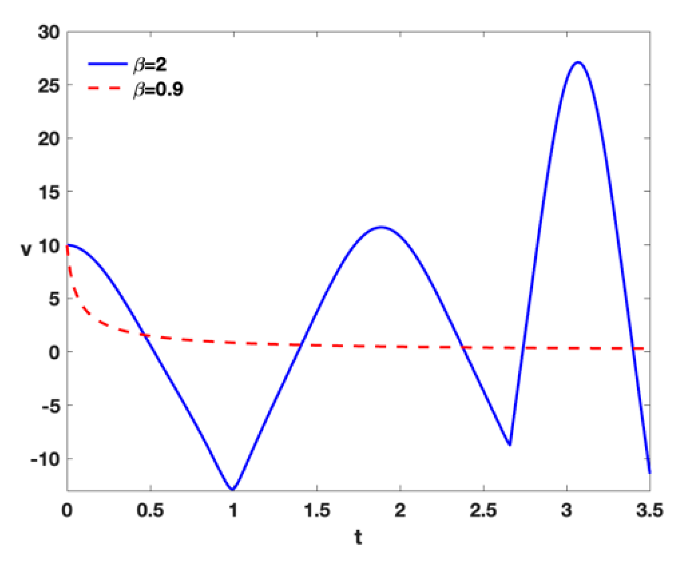
In order to illustrate the expediency of using the fractal approach in comparison with the integer approach, Figure 9 shows that the integer approach is not practical, and the tumor cells are still growing with $\beta =2$, but the fractional approach is more realistic at this point and the number of tumor cells drops dramatically.

5. Conclusions

In this paper, we have investigated a fractional-order tumor–immune interaction model with immunotherapy and B-D functional response function. First, we obtain the existence, uniqueness, and nonnegativity of the solutions of the model (Equation (1)) (see Theorems 1 and 2). Second, there are some equilibrium points, depending on what treatment is not used and whether the tumor is curable. Moreover, the local asymptotic stability of these equilibrium points is proved by using the Hurwitz conditions and the linearization method (see Theorems 3–6), which means that the tumor cells can be destroyed or controlled by using immunotherapy. Then, sufficient conditions for the global asymptotic stability of the unique positive equilibrium are proved by using the method of the Lyapunov function (see Theorem 7). Finally, we visualized the theorem presented in this paper by numerical simulation. The numerical simulation results show that the equilibrium points can reach local or global asymptotic stability, which indicates that under certain conditions, the tumor can be completely cured or effectively controlled, respectively. For the fractional-order equation used in this paper, the larger the value of $\beta$, the faster and better the tumor will be cured or controlled. At present, the numerical simulation is still in the verification stage of theoretical results, and the simulation analysis has not involved real data. It is hoped that the real data can be better combined with theoretical research in the future, so as to achieve the effect of tumor suppression more efficiently.

References

1. Kawaguchi, K.; Maeshima, Y.; Toi, M. Tumor immune microenvironment and modelic response in breast cancer. Med. Oncol. 2022, 19, 1–10. [Google Scholar]
2. Wu, Z.; Zhang, C.; Najafi, M. Targeting of the tumor immune microenvironment by metformin. J. Cell Commun. Signal. 2021, 16, 333–348. [Google Scholar] [CrossRef] [PubMed]
3. Bashkirtseva, I.; Chukhareva, A.; Ryashko, L. Modeling and analysis of nonlinear tumor-immune interaction under chemotherapy and radiotherapy. Math. Methods Appl. Sci. 2021, 45, 7983–7991. [Google Scholar] [CrossRef]
4. Lee, H.; Na, K.J.; Choi, H. Didderences in Tumor Immune Microenvironment in Matastatic Sites of Breast Cancer. Front. Oncol. 2021, 11, 722. [Google Scholar]
5. Ko, W.; Ahn, I. Stationary patterns and stability in a tumor-immune interaction model with immunotherapy. J. Math. Anal. Appl. 2011, 383, 307–329. [Google Scholar] [CrossRef] [Green Version]
6. Han, L.; Messan, M.R.; Yogurtcu, O.N.; Nukala, U.; Yang, H. Analysis of tumor-immune functional responses in a mathematical model of neoantigen cancer vaccines. Math. Biosci. 2023, 356, 108966. [Google Scholar] [CrossRef] [PubMed]
7. Zhou, Q.; Yan, Y.; Li, Y.; Fu, H.; Lu, D.; Li, Z.; Wang, Y.; Wang, J.; Zhu, H.; Ren, J.; et al. Tumor-derived extracellular vesicles in melanoma immune response and immunotherapy. Biomed. Pharmacother. 2022, 156, 113790. [Google Scholar] [CrossRef] [PubMed]
8. Kirschner, D.; Panetta, J.C. Modeling immunotherapy of the tumor—Immune interaction. J. Math. Biol. 1998, 37, 235–252. [Google Scholar] [CrossRef] [PubMed] [Green Version]
9. Yang, W.; Feng, X.; Liang, S.; Wang, X. Asymptotic Behavior Analysis of a Fractional-Order Tumor-Immune Interaction Model with Immunotherapy. Complexity 2020, 2020, 7062957. [Google Scholar] [CrossRef]
10. Petráš, I. Fractional-Order Nonlinear Models: Modeling, Analysis and Simulation; Springer Science & Business Media: Berlin, Germany, 2011. [Google Scholar]
11. Kilbas, A.A.A.; Srivastava, H.M.; Trujillo, J.J. Theory and Applications of Fractional Differential Equations; Elsevier Science Limited: Amsterdam, The Netherlands, 2006; Volume 204. [Google Scholar]
12. Beddington, J.R. Mutual Interference Between Parasites or Predators and its Effect on Searching Efficiency. J. Anim. Ecol. 1975, 44, 331. [Google Scholar] [CrossRef] [Green Version]
13. DeAngelis, D.; Goldstein, R.A.; Neill, R.V.O. A model for trophic interaction. Ecology 1975, 56, 881–892. [Google Scholar] [CrossRef]
14. Li, H.-L.; Zhang, L.; Hu, C.; Jiang, Y.-L.; Teng, Z. Dynamical analysis of a fractional-order predator-prey model incorporating a prey refuge. J. Appl. Math. Comput. 2016, 54, 435–449. [Google Scholar] [CrossRef]
15. Li, Y.; Chen, Y.; Podlubny, I. Stability of fractional-order nonlinear dynamic models: Lyapunov direct method and generalized Mittag-Leffler stability. Comput. Math. Appl. 2010, 59, 1810–1821. [Google Scholar] [CrossRef] [Green Version]
16. Choi, S.K.; Kang, B.; Koo, N. Stability for caputo fractional differential model. Abstr. Appl. Anal. 2014, 2014, 631419. [Google Scholar] [CrossRef] [Green Version]
17. Pao, C.V. Nonlinear Parabolic and Elliptic Equations; Plenum Press: New York, NY, USA, 1992. [Google Scholar]
18. Clark, R.N. The Routh-Hurwitz stability criterion, revisited. IEEE Control Syst. 1992, 12, 119–120. [Google Scholar] [CrossRef] [Green Version]
19. Vargas-De-León, C. Voletrra-type Lyapunov functions for fractional-order epidemic systems. Commun. Nonlinear Sci. Numer. Simul. 2015, 24, 75–85. [Google Scholar] [CrossRef]
20. Aguila-Camacho, N.; Duarte-Mermoud, M.A.; Gallegos, J.A. Lyapunov functions for fractional order systems. Commun. Nonlinear Sci. Numer. Simul. 2014, 19, 2951–2957. [Google Scholar] [CrossRef]
21. Diethelm, K.; Ford, N.J.; Freed, A.D. A Predictor-Corrector Approach for the Numerical Solution of Fractional Differential Equations. Nonlinear Dyn. 2002, 29, 3–22. [Google Scholar] [CrossRef]
22. Garrappa, R. Trapezoidal methods for fractional differential equations: Theoretical and computational aspects. Math. Comput. Simul. 2013, 110, 96–112. [Google Scholar] [CrossRef] [Green Version]
Figure 1. Time series (a) and phase diagram (b) of equilibrium point A 2 = ( 3 , 0 , 0 ) with a = 0.9 , m 1 = 1 , k 1 = 0.5 , b = 1 , c = 3 , s 1 = 3 , d = 2.5 , k 2 = 1 , m 2 = 1 , s 2 = 0 , and β = 0.9 .
Fractalfract 07 00200 g001
Figure 2. Time series (a) and phase diagram (b) of equilibrium point A 4 = ( 4 , 0 , 1 ) with a = 0.9 , m 1 = 1 , k 1 = 0.5 , b = 1 , c = 3 , s 1 = 3 , d = 2.5 , k 2 = 1 , m 2 = 1 , s 2 = 1 , and β = 0.9 .
Fractalfract 07 00200 g002
Figure 3. Time series of model (Equation (1)) with a = 0.9 , m 1 = 1 , k 1 = 0.5 , b = 1 , c = 3 , d = 2.5 k 2 = 1 , m 2 = 1 , s 1 = 3 and different values of β . (a) s 2 = 0 and (b) s 2 = 1 .
Fractalfract 07 00200 g003
Figure 4. Time series of tumor cells with a = 0.9 , m 1 = 1 , k 1 = 0.5 , b = 1 , c = 3 , d = 2.5 , k 2 = 1 , m 2 = 1 , s 2 = 0 and different treatment by different densities of s 1 .
Fractalfract 07 00200 g004
Figure 5. Time series of tumor cells with a = 0.9 , m 1 = 1 , k 1 = 0.5 , b = 1 , c = 3 , d = 2.5 , k 2 = 1 , m 2 = 1 , s 1 = 3 and different treatment by the different densities of s 2 .
Fractalfract 07 00200 g005
Figure 6. Time series of tumor cells with a = 0.9 , m 1 = 1 , k 1 = 0.5 , b = 1 , c = 3 , d = 2.5 , k 2 = 1 , m 2 = 1 , s 1 = 3 and different treatment by higher different densities of s 2 .
Fractalfract 07 00200 g006
Figure 7. Time series (a) and phase diagram (b) of equilibrium point A ^ = ( 1.11 , 0.51 , 1.64 ) with a = 0.9 , m 1 = 1 , k 1 = 0.5 , b = 1 , c = 3 , s 1 = 0.3 , d = 5 , k 2 = 1 , m 2 = 1 , s 2 = 1.5 , and β = 0.9 .
Fractalfract 07 00200 g007
Figure 8. Phase diagram of equilibrium point A ^ = ( 1.11 , 0.51 , 1.64 ) with a = 0.9 , m 1 = 1 , k 1 = 0.5 , b = 1 , c =   3 , s 1 = 0.3 , d = 5 , k 2 = 1 , m 2 = 1 , s 2 = 1.5 , β = 0.9 , and different initial conditions ( u 0 , v 0 , w 0 ) . The initial conditions of the blue, red and green lines are ( u 0 , v 0 , w 0 ) = ( 4 , 4 , 4 ) , ( u 0 , v 0 , w 0 ) = ( 3 , 3 , 3 ) and ( u 0 , v 0 , w 0 ) = ( 2 , 2 , 2 ) respectively.
Fractalfract 07 00200 g008
Figure 9. Time series of tumor cells with a = 0.9 , m 1 = 1 , k 1 = 0.5 , b = 1 , c = 3 , d = 2.5 , k 2 = 1 , m 2 = 1 , s 1 = 3 , s 2 = 1 and different treatment by higher different densities of β .
Fractalfract 07 00200 g009
Disclaimer/Publisher’s Note: The statements, opinions and data contained in all publications are solely those of the individual author(s) and contributor(s) and not of MDPI and/or the editor(s). MDPI and/or the editor(s) disclaim responsibility for any injury to people or property resulting from any ideas, methods, instructions or products referred to in the content.