Article

Numerical Solutions of the (2+1)-Dimensional Nonlinear and Linear Time-Dependent Schrödinger Equations Using Three Efficient Approximate Schemes

by
Neveen G. A. Farag
1,*,
Ahmed H. Eltanboly
1,2,
Magdi S. El-Azab
1 and
Salah S. A. Obayya
3,4
1
Mathematics and Engineering Physics Department, Faculty of Engineering, Mansoura University, Mansoura 35516, Egypt
2
Mathematics Department, Faculty of Science, Galala University, Suez 435611, Egypt
3
Centre for Photonics and Smart Materials, Zewail City of Science and Technology, October Gardens, 6th of October City, Giza 12578, Egypt
4
Electronics and Communications Engineering Department, Faculty of Engineering, Mansoura University, Mansoura 35516, Egypt
*
Author to whom correspondence should be addressed.
Fractal Fract. 2023, 7(2), 188; https://doi.org/10.3390/fractalfract7020188
Submission received: 20 December 2022 / Revised: 31 January 2023 / Accepted: 9 February 2023 / Published: 13 February 2023

Abstract

:
In this paper, the (2+1)-dimensional nonlinear Schrödinger equation (2D NLSE) abreast of the (2+1)-dimensional linear time-dependent Schrödinger equation (2D TDSE) are thoroughly investigated. For the first time, these two notable 2D equations are attempted to be solved using three compelling pseudo-spectral/finite difference approaches, namely the split-step Fourier transform (SSFT), Fourier pseudo-spectral method (FPSM), and the hopscotch method (HSM). A bright 1-soliton solution is considered for the 2D NLSE, whereas a Gaussian wave solution is determined for the 2D TDSE. Although the analytical solutions of these partial differential equations can sometimes be reached, they are either limited to a specific set of initial conditions or even perplexing to find. Therefore, our suggested approximate solutions are of tremendous significance, not only for our proposed equations, but also to apply to other equations. Finally, systematic comparisons of the three suggested approaches are conducted to corroborate the accuracy and reliability of these numerical techniques. In addition, each scheme’s error and convergence analysis is numerically exhibited. Based on the MATLAB findings, the novelty of this work is that the SSFT has proven to be an invaluable tool for the presented 2D simulations from the speed, accuracy, and convergence perspectives, especially when compared to the other suggested schemes.

1. Introduction

The Schrödinger equation is a classical field equation. Its vitality is due to its principal applications in simulating the light propagation in nonlinear optical fibers and planar waveguides in quantum mechanics [1]. Therefore, this study is devoted to approximating two prestigious variants of Schrödinger equations, which are the two-dimensional cubic nonlinear Schrödinger equation (2D NLSE) and the two-dimensional time-dependent Schrödinger equation (2D TDSE), using three powerful approaches, which are the SSFT, FPSM, and HSM. The first two methods belong to the pseudo-spectral family while the last scheme is a finite difference method. These methods were initially introduced by Taha and Ablowitz [2] in 1984 to approximate the one-dimensional nonlinear Schrödinger equation (1D NLSE). Since then, they have been widely applied to solve other types of significant partial differential equations. The 1D NLSE, from which the 2D NLSE is derived, is a central model of nonlinear science that describes a wide class of phenomena, for example, modulational instabilities of water waves [3], propagation of heat pulses in anharmonic crystals, nonlinear modulation of collisionless plasm waves, helical motion of a very thin vortex filament, self-trapping of a light beam in a color-dispersive system, and so forth [2]. Its numerical solutions have been widely explored by numerous researchers for their importance in a plethora of mathematical and physical systems. Likewise, much effort has been specifically dedicated to investigating its analytical solutions, such as the Akhmediev breathers [3], Kuznetsov–Ma solitons [4,5], Peregrin soliton [6], and rouge waves (RWs), which are currently a hot topic of research [7,8]. Furthermore, even in the quantum optics [9] new RW excitations have been analyzed [10].
To kick off, the well-known 2D NLSE is considered, which has a crucial contribution in modeling a broad range of physical phenomena, such as nonlinear optics, plasma physics, electromagnetic wave propagation, underwater acoustics, Bose–Einstein condensation, biomolecule dynamics, protein chemistry, and design of optoelectronic devices. This equation is framed as [11,12,13,14,15]:
i Ψ x , y , t t + 2 x 2 + 2 y 2 Ψ x , y , t + β Ψ x , y , t 2 Ψ x , y , t = 0 ,   x , y , t Ω × 0 , T
Subject to the initial condition and boundary conditions given by:
Ψ x , y , 0 = Ψ 0 x , y ,                                 x , y Ω
Ψ x , y , t = 0 ,           x , y Γ ,                 0 t T
In Equation (1), Ψ x , y , t is a complex-valued function that indicates the complex amplitude of the waveform, where x , y , and t denote spatial and temporal variables, respectively, 2 x 2 + 2 y 2 is the Laplacian operator, Ω is [ x l ,   x r × y l ,   y r ], Γ is the boundary of Ω , and β is a real constant. Despite the presence of the analytical solution of this equation, it is only limited to a specific set of initial conditions [16,17,18,19,20]. Therefore, numerous researchers have potentially exerted nontrivial efforts attempting to seek creditable approximate solutions for this significant equation, such as the finite difference method, finite element method, discontinuous Galerkin method, meshless method, finite difference method, spectral and pseudo-spectral method, and so forth. This can be found in [12,21] and references therein. In recent years, a plethora of finite difference schemes alongside copious pseudo-spectral approaches have been competently utilized and corroborated to be unconditionally stable and convergent in solving the NLS equation in multi-dimensions with the optimal rate of convergence [11,12]. However, our presented schemes are seldom used.
Likewise, we address the eminent 2D TDSE that is deemed to be the central equation in quantum mechanics. In specific, it is exhaustively used in modeling quantum devices, propagation of electromagnetic waves, and design of optoelectronic devices. Moreover, it mainly depends on one temporal variable and two spatial ones, which slightly resemble the formulation of the 2D NLSE, as shown below [22,23,24,25]:
i Ψ x , y , t t + 2 x 2 + 2 y 2 Ψ x , y , t + V x , y , t Ψ x , y , t = 0 ,   x , y , t Ω × 0 , T
For Equation (4), the initial and boundary conditions are the same as demonstrated in Equations (2) and (3). The equation’s parameters are similar to what we have previously defined for the 2D NLSE, whereas V x , y , t is a real-valued function that describes the trapping potential of the energy function. More importantly, this outstanding equation is frequently used to simulate the propagation of the electron wave through the quantum wire. However, to model the dynamics of the electron wave propagating along the z-direction through a quantum wire, the two-dimensional time-dependent linear Schrödinger equation is evoked in its modified form, which is compatible with the electron waveguide parameters, as exhibited below [26,27,28]:
ћ 2 2 m 2 x 2 + 2 y 2 + U x , y E Ψ x , y , t = i ћ Ψ x , y , t t ,                                 x , y , t Ω × 0 , T
where Ψ x , y , t is the wave function of the electron, m is the effective mass, ћ is the plank’s constant divided by 2π, t is the time, U is the potential energy, and E is the energy. Due to the ultimate importance of this equation in the quantum mechanics realm, it has widely been explored using plenty of numerical techniques seeking a precise solution for this equation. For instance, collocation and radial basis functions, the meshless symplectic method, extended Boadway’s transformation technique, meshless symplectic procedure are based on highly accurate multiquadric quasi-interpolation and many more. For more details, see [22,23,24,25,26,27,28]. Nowadays, plenty of significant partial differential equations, such as the 2D NLSE and 2D TDSE have efficiently been solved employing either a finite difference method or a pseudo-spectral approach, such as the Gross–Pitaevskii equation [29], the complex Ginzburg Landau equation [30], 2D distributed-order time-fractional cable equation [31], variable-coefficient Korteweg–De Vries equation [32], and many others [33,34,35]. In this literature, both theoretical analysis and numerical simulation are comprehensively demonstrated.
Here, this work’s main goal is to seek plausible simulations for the processes described by two distinguished partial differential equations, which are the 2D NLSE abreast of the 2D TDSE. Our target cannot easily be achieved because most partial differential equations (PDEs) are notoriously difficult to be analytically solved. Therefore, numerous works in literature have recently been dedicated to a plethora of numerical approaches in an attempt to tackle the crucial physical and engineering phenomena, modeled by partial differential equations [36]. In this paper, three approximate numerical schemes are presented, for the first time, to report these two equations; two of them belong to the pseudo-spectral methods, which are the SSFT and the FPSM, whereas the last one is a finite difference method, which is called the HSM. A bright soliton solution is obtained for the 2D NLSE, while a Gaussian wave solution is constructed for the 2D TDSE. The verification is performed by comparing our suggested schemes with their exact analytical solution and the results are exhibited in the form of both tables and graphs. Error and convergence analyses are also explored numerically. In our future work, this study could be beneficial in providing a profound insight into the process of solving other partial differential equations that might describe plenty of significant real-life applications.
This paper is organized as follows. Following this brief introduction addressing the 2D NLSE and 2D TDSE, Section two demonstrates the mathematical preliminaries of the suggested numerical approaches for approximating the 2D NLSE followed by the 2D TDSE. The numerical assessments and discussion are elaborated upon in Section three. Finally, Section four culminates in the overall conclusion of the entire study.

2. Mathematical Preliminaries

Here, we extend the work presented in [2,30,33] to two important variants of the (2+1)-dimensional Schrödinger equation. To be precise, this section fosters two major parts. First, the three proposed numerical schemes, which are the SSFT, FPSM, and HSM, are exhibited for reporting the 2D NLSE alongside its analytical solution. Second, the theoretical analysis of each of these methods is established in order to cope with the structure of the 2D TDSE.

2.1. (2+1)-Dimensional Nonlinear Schrödinger Equation (2D NLSE)

The 2D NLSE described in Equation (1) is recalled in this subsection along with its exact bright 1-soliton solution [16,21,37], as shown below:
Ψ x , y , t = ( 2 λ ) 0.5 e i k 1 x + k 2 y + ω t + Φ o s e c h   ( λ ) 0.5 x + y c t + x o
where, x o ,   Φ o ,   c ,   λ   are the initial position, initial phase, propagation speed, and soliton amplitude, respectively.
Following this, the three compelling numerical techniques are implemented to solve the 2D NLSE.

2.1.1. Method 1: Split-Step Fourier Transform Method

This scheme is unpretentious, expedient, accurate, and unconditionally stable. Its unique strategy for the solution relies on the concept of splitting the PDE into two sequential linear and nonlinear partial equations.
In this regard, Equation (1) should be rearranged in the form of Ψ x , y , t t = L + N Ψ x , y , t , which yields:
Ψ x , y , t t = i 2 x 2 + 2 y 2 Ψ x , y , t + β i Ψ x , y , t 2 Ψ x , y , t            
First, we introduce the nonlinear step over a small interval of time [ t ,   t + Δ t ] , as follows: Ψ x , y , t t = N Ψ . Where the nonlinear operator is given by: N = β i Ψ x , y , t 2 . Therefore, the analytical solution of the nonlinear step at time t = t + Δ t   will be given by the following equation, where Δ t is the temporal step size [38]:
Ψ x , y , t + Δ t = e x p Δ t N Ψ x , y , t = e x p   β i Δ t Ψ x , y , t 2 Ψ x , y , t
Second, define the linear step: i Ψ x , y , t t = L Ψ . Where the linear operator is depicted by: L = i 2 x 2 + 2 y 2 . Then, we apply the Fourier transform to both sides, which can easily be solved, as follows:
Ψ ^ x , y , t t = i ω 2 + ν 2 Ψ ^
Thus, the analytical solution of the preceding equation is exhibited, as follows:
Ψ ^ x , y , t + τ = e x p i ω 2 + ν 2 Δ t . Ψ ^ x , y , t )
Finally, the final equation in the time domain can be formulated, as shown below, where F and F 1 denote the Fourier and inverse Fourier transforms, respectively [38]. In a numerical analysis, these transforms can efficiently be performed with the fast Fourier transform algorithm [2]:
Ψ x , y , t + Δ t = F 1 ( e x p i ω 2 Δ t . e x p i ν 2 Δ t . F e x p β i Δ t Ψ x , y , t 2 Ψ x , y , t )

2.1.2. Method 2: Fourier Pseudo-Spectral Method

The rudimentary basis of this pseudo-spectral approach leans on applying the Fourier transform to the second-order derivatives while employing the finite-difference relations to discretize the first-order time derivative. This technique is unconditionally stable. Additionally, it should be applied to periodic functions over a domain Ω P , P × P ,   P .
Firstly, replacing the temporal first derivative with the following difference relation
Ψ t = Ψ x , y , t + Δ t Ψ x , y , t Δ t
Secondly, substituting Equation (12) into Equation (1) leads to the following equations,
Ψ x , y , t + Δ t Ψ x , y , t Δ t = F 1 ( i 2 ω 2 π 2 P 2 F Ψ ) F 1 ( i 2 ν 2 π 2 P 2 F Ψ ) β Ψ x , y , t 2 Ψ x , y , t
Ψ x , y , t + Δ t Ψ x , y , t = i Δ t F 1 ( i 2 ω 2 π 2 P 2 F Ψ ) + i Δ t F 1 ( i 2 ν 2 π 2 P 2 F Ψ ) + i Δ t β Ψ x , y , t 2 Ψ x , y , t
Ψ x , y , t + Δ t = Ψ x , y , t Δ t i F 1 ( ω 2 π 2 P 2 F Ψ ) ) Δ t i F 1 ( i 2 ν 2 π 2 P 2 F Ψ ) + i Δ t β Ψ x , y , t 2 Ψ x , y , t
The previous equation provides a solution, which is only stable for values of Δ t Δ x 2 < 1 π 2 and Δ t Δ y 2 < 1 π 2 .
However, adjusting the previous equation, by using the Fornberg and Whitham principles, leads to an unconditionally stable solution, as shown in the equation below:
Ψ x , y , t + Δ t = Ψ x , y , t i F 1 ( s i n ω 2 π 2 P 2 Δ t F Ψ x , y , t ) i F 1 ( s i n ν 2 π 2 P 2 Δ t F Ψ x , y , t ) +   i Δ t β Ψ x , y , t 2 Ψ x , y , t

2.1.3. Method 3: Hopscotch Method

This explicit finite difference method is deemed to be a rapid and unconditionally stable approach that counts on discretizing the space and time derivatives using appropriate difference relations. However, at approximates the nonlinear term of the equation using an average formula as is exhibited below:
Ψ i j = Ψ i 1 , j 2 Ψ i 1 , j + Ψ i + 1 , j 2 Ψ i + 1 , j 2
Subsequently, we plug the previous equation, which is computed at the row j , and the other appropriate difference relations in Equation (1), subject to the boundary and initial conditions, which yields:
i Ψ i , j + 1 Ψ i , j Δ t + Ψ i + 1 , j + Ψ i 1 , j 2 Ψ i , j Δ x 2 + Ψ i + 1 , j + Ψ i 1 , j 2 Ψ i , j Δ y 2 + β Ψ i 1 , j 2 Ψ i 1 , j + Ψ i + 1 , j 2 Ψ i + 1 , j 2 = 0
i Ψ i , j + 1 Ψ i , j = Δ t Ψ i + 1 , j + Ψ i 1 , j 2 Ψ i , j Δ x 2 Δ t Ψ i + 1 , j + Ψ i 1 , j 2 Ψ i , j Δ y 2 Δ t β Ψ i 1 , j 2 Ψ i 1 , j + Ψ i + 1 , j 2 Ψ i + 1 , j 2
Ψ i , j + 1 = Ψ i , j + i Δ t Ψ i + 1 , j + Ψ i 1 , j 2 Ψ i , j Δ x 2 + i Δ t Ψ i + 1 , j + Ψ i 1 , j 2 Ψ i , j Δ y 2 + i β Δ t 2 ( Ψ i 1 , j 2 Ψ i 1 , j + Ψ i + 1 , j 2 Ψ i + 1 , j )
Thus, the below equation provides the final explicit formula, where λ = Δ t Δ x 2 and λ * = Δ t Δ y 2 ,
Ψ i , j + 1 = 1 2 i ( λ + λ * ) Ψ i , j + i λ + λ * Ψ i + 1 , j + Ψ i 1 , j + i β Δ t 2 Ψ i 1 , j 2 Ψ i 1 , j + Ψ i + 1 , j 2 Ψ i + 1 , j

2.2. (2+1)-Dimensional Time-Dependent Linear Schrödinger Equation (2D TDSE)

In this section, our numerical approaches are applied to the 2D TDSE, which is the governing equation of the quantum wire. More precisely, this significant equation mimics the electron wave motion through the electron waveguide.
Furthermore, we rewrite the 2D TDSE, as shown in Equation (5), in a more compact form to obtain Equation (22), as elaborated below:
ξ 2 x 2 + 2 y 2 + η Ψ x , y = i Ψ x , y t ξ = ћ 2 m ,                         η = U x , y E ћ
A general analytical solution is considered associated with this equation based on the separation of variables technique:
Ψ x , y , t = Ψ 0 x , y e i E t ћ

2.2.1. Method 1: Split-Step Fourier Transform Approach

We begin with Equation (22), which is already framed in the form of: Ψ x , y , t t = L + N Ψ x , y , t .
Knowing that the linear operator is defined as L = i ξ 2 x 2 + 2 y 2 + η , whereas the nonlinear operator is absent from this equation, such that N = 0 .
Therefore, the nonlinear step, which is given by Ψ x , y , t t = N Ψ x , y , t , has an analytical solution of the form:
Ψ x , y , t + Δ t = e x p i Δ t N Ψ x , y , t
Ψ x , y , t + Δ t = Ψ x , y , t
While the linear step, which is represented by Ψ x , y , t t = L Ψ x , y , t , is transformed from the time domain into the frequency domain, as follows:
  Ψ ^   x , y , t t = i ξ ω 2 + ν 2 + i η Ψ ^
Its analytical solution is given in the frequency domain, as demonstrated below:
Ψ ^ ω , ν , t + Δ t = e x p i ξ ω 2 Δ t . e x p i ξ ν 2 Δ t . e x p i η Δ t . Ψ ^ ω , ν , t
Hence, the approximate solution can be written as:
Ψ x , y , t + Δ t = F 1 ( e x p i ξ ω 2 Δ t . e x p i ξ ν 2 Δ t . e x p i η Δ t . F Ψ x , y , t )

2.2.2. Method 2: Fourier Pseudo-Spectral Method

Substituting the temporal difference relation, presented in Equation (12), into Equation (22) to obtain the following equations:
i Ψ x , y , t + Δ t Ψ x , y , t Δ t = F 1 ( i 2 ω 2 π 2 P 2 F Ψ ) F 1 ( i 2 ν 2 π 2 P 2 F Ψ ) + η Ψ x , y , t
Ψ x , y , t + Δ t Ψ x , y , t = ξ i Δ t F 1 ( i 2 ω 2 π 2 P 2 F Ψ ) + ξ i Δ t F 1 ( i 2 ν 2 π 2 P 2 F Ψ ) i Δ t η Ψ x , y , t
Ψ x , y , t + Δ t = Ψ x , y , t ξ Δ t i F 1 ( ω 2 π 2 P 2 F Ψ ) ξ Δ t i F 1 ( ν 2 π 2 P 2 F Ψ ) i Δ t η Ψ x , y , t
Incorporating the Fornberg and Whitham principles, in the preceding formula, leads to an unconditionally stable solution, as shown in the equation below:
Ψ x , y , t + Δ t = Ψ x , y , t i ξ F 1 ( s i n ω 2 π 2 P 2 Δ t F Ψ x , y , t ) i ξ F 1 ( s i n ν 2 π 2 P 2 Δ t F Ψ x , y , t ) i η Δ t Ψ x , y , t

2.2.3. Method 3: Hopscotch Method

The basic step that differentiates this scheme from the previously illustrated HSM is to approximate the linear term, presented in Equation (22), using the average relation shown below:
Ψ i j = Ψ i 1 , j + Ψ i + 1 , j 2
Then, replacing the first and second-order derivatives using the appropriate difference relations demonstrated earlier, to obtain the below equations:
i Ψ i , j + 1 Ψ i , j Δ t = ξ Ψ i + 1 , j + Ψ i 1 , j 2 Ψ i , j Δ x 2 ξ Ψ i + 1 , j + Ψ i 1 , j 2 Ψ i , j Δ y 2 + η Ψ i 1 , j + Ψ i + 1 , j 2
i Ψ i , j + 1 Ψ i , j + ξ Δ t Ψ i + 1 , j + Ψ i 1 , j 2 Ψ i , j Δ x 2 + ξ Δ t Ψ i + 1 , j + Ψ i 1 , j 2 Ψ i , j Δ y 2 η Δ t Ψ i 1 , j + Ψ i + 1 , j 2 = 0
Ψ i , j + 1 = Ψ i , j + i ξ Δ t Ψ i + 1 , j + Ψ i 1 , j 2 Ψ i , j Δ x 2 + i ξ Δ t Ψ i + 1 , j + Ψ i 1 , j 2 Ψ i , j Δ y 2 i η Δ t Ψ i 1 , j + Ψ i + 1 , j 2
Thus, the following equation provides the final explicit formula, where λ = Δ t Δ x 2 and λ * = Δ t Δ y 2 ,
Ψ i , j + 1 = 1 2 i ξ ( λ + λ * ) Ψ i , j + i ξ λ + λ * Ψ i + 1 , j + Ψ i 1 , j i η Δ t Ψ i 1 , j + Ψ i + 1 , j 2

3. Numerical Experiments

This section is oriented to comprise two consecutive numerical assessments. The first one pertains to the solution of the 2D NLSE using the three suggested schemes named SSFT, FPSM, and HSM whereas comparing their obtained results with the exact solution to corroborate their accuracy, stability, and convergence. The second assessment targets the 2D TDSE solutions. Specifically, the three proposed techniques are managed to extract the approximate solution of the 2D TDSE. Thereafter, the approximate solutions of the three schemes are compared with their analytical solution as well to substantiate their effectiveness.

3.1. Simulations of the 2D NLSE

To perform this experiment, we have employed an initial bright soliton of the form:
Ψ 0 x , y = ( 2 ) 0.5 e i k 1 x + k 2 y s e c h   x + y
The preceding equation has been attained by plugging λ and c equal to one while setting Φ o and x o to zero in Equation (6).
In the meantime, we have carried out our experiment with β = 1 plugged in Equation (1), representing the 2D NLSE, over a square physical domain Ω = [−20, 20] × [−20, 20], which is uniformly discretized with a grid composed of 201 × 201 points, under a temporal precision of Δ t = 10   × 10 3 and spatial precision of Δ x = Δ y = 2 × 10 1 . We have opted for these selections, taking into consideration that the smaller the values of spatial and temporal step sizes that we select, the higher the accuracy of the scheme due to the greater number of grid points we obtain for the computations. However, because of the additional complexity, the computational process takes longer to execute. At the first stage of this test, we have recorded the absolute values of the wave amplitude at a specific time t = 1 that is executed through 1001 subsequent iterations, while utilizing random x values from the interval [1, 10] and y values from the interval [5, 15]. These wave amplitudes are computed based on the three proposed numerical approaches, along with the exact solution, presented in Equation (6), to advocate for their accuracy and stability. All of these computed values are extensively summarized in Table 1.
In addition, a 3D graph of the modulus of the exact analytical solution of the 2D NLSE, employing a bright soliton has been exhibited in Figure 1. This solution has been computed over x and y domains of [−20, 20] × [−20, 20] at time t = 10 . Moreover, the SSFT method has been implemented to solve Equation (1) over x and y domains of [−30, 30] × [−30, 30] at a time sequence of t = 1 , t = 3 , and t = 6 . This process has resulted in discretizing the square physical domain into an equally spaced grid of 301 × 301 points, while executing the different values of time required for the consecutive software iterations of 1001, 3001, and 6001, respectively. The dynamic behavior of the obtained results is demonstrated in Figure 2. Specifically, the 3D graphs are presented in Figure 2a–c, whereas Figure 2d–f represent the 2D graphs of the resulted approximate solution. The corresponding contour plots are clearly shown in Figure 2g–i.

3.1.1. Error and Convergence Analysis

Subsequently, the second stage of this experiment is to compute the error, represented in calculating the sum of squares error (SSE) and thus conduct an exhaustive comparison among our proposed numerical approaches, against their exact analytical solution, over the same equal domain of x and y values from −20 to 20, but at different values of time from 0.1 to 2. For this test, we have used a temporal step size of 10 3 and spatial step size of 2 × 10 1 for all of the proposed approaches as well. The SSE has been recorded at each time value to manifest the difference between the exact and the approximate solution. Table 2 demonstrates the SSEs for the three proposed methods abreast of the CPU processing time in seconds.
Finally, to numerically advocate the convergence of the proposed numerical schemes, three graphs have been developed and further demonstrated in Figure 3. These graphs illustrate the relationship between a set of different temporal step sizes versus the absolute error, computed by u e u a / u a , where u e is the exact solution while ua represents the approximate solution. In Figure 3a, the SSFT has been employed over a square domain of [−20, 20] × [−20, 20] while changing the temporal step size from 0.0005 to 0.0095. This experiment has been performed at consecutive times of t = 3 ,   5 ,   and   7 . The same values have been used for the FPSM in. Figure 3b. Whereas in Figure 3c, the HSM has been applied over a square domain of [−10, 10] × [−10, 10], temporal range values from 0.0001 to 0.0009, and performed at time values of t = 1 ,   1.5 ,   and   2 to reduce the execution time.

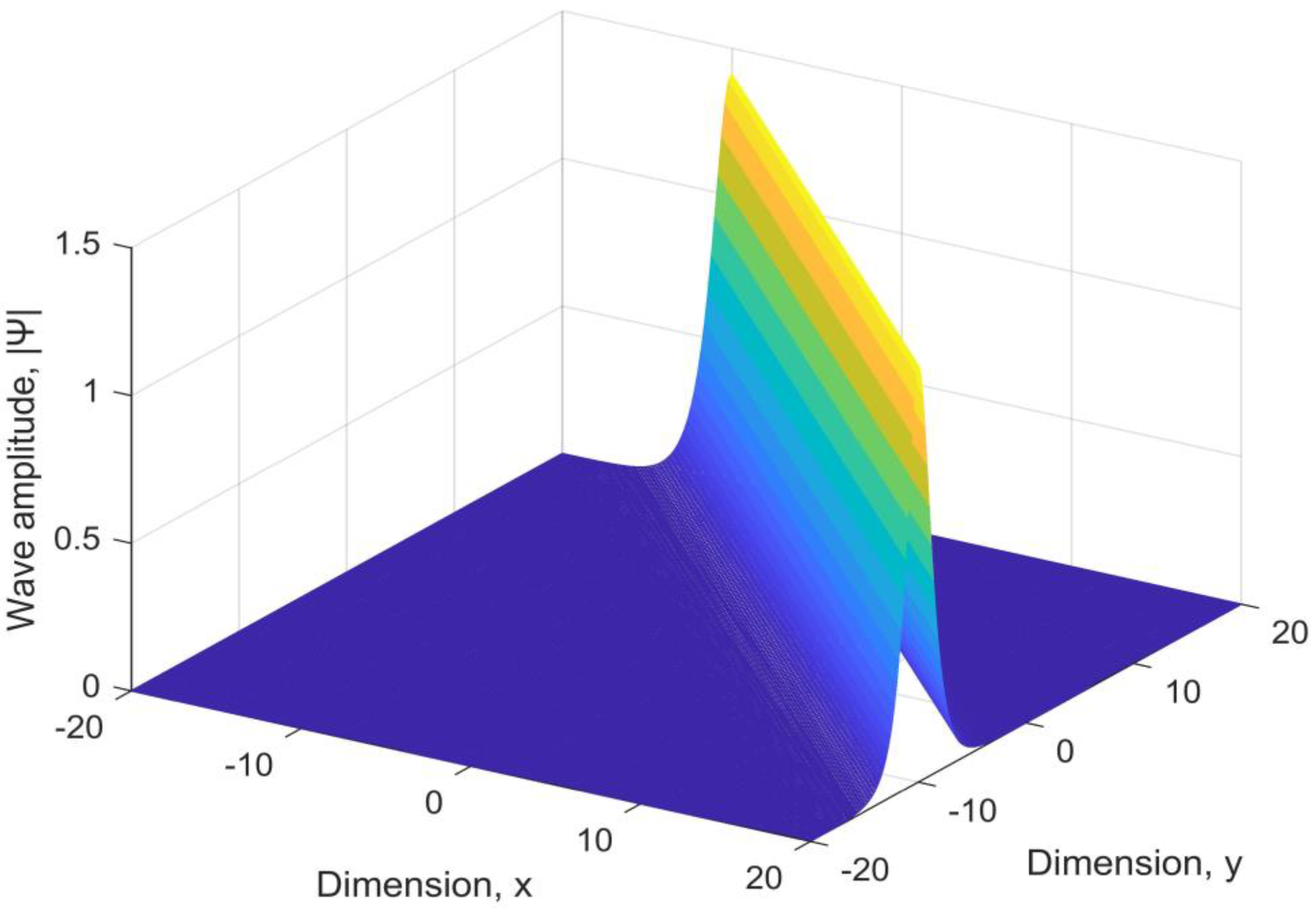
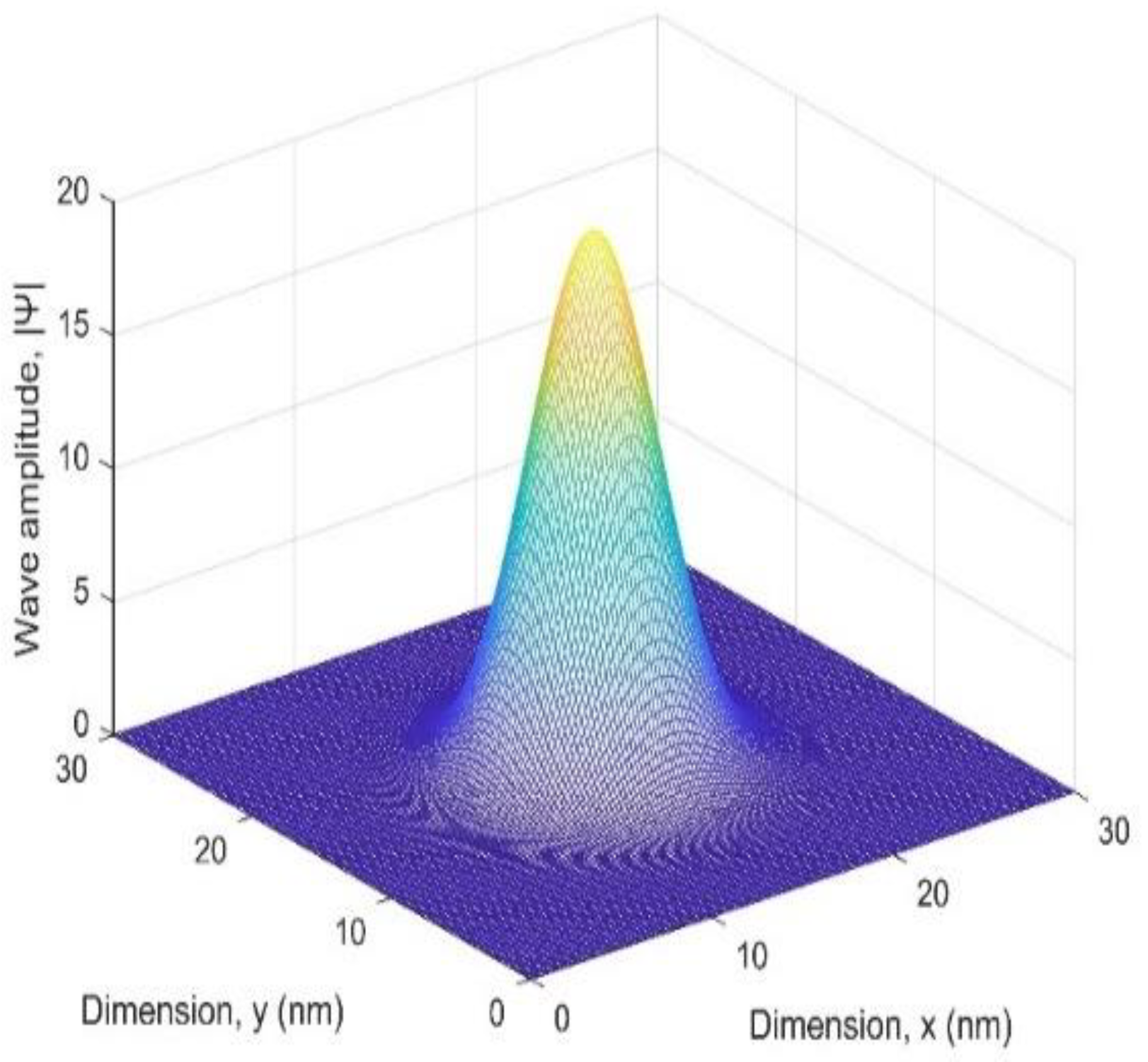
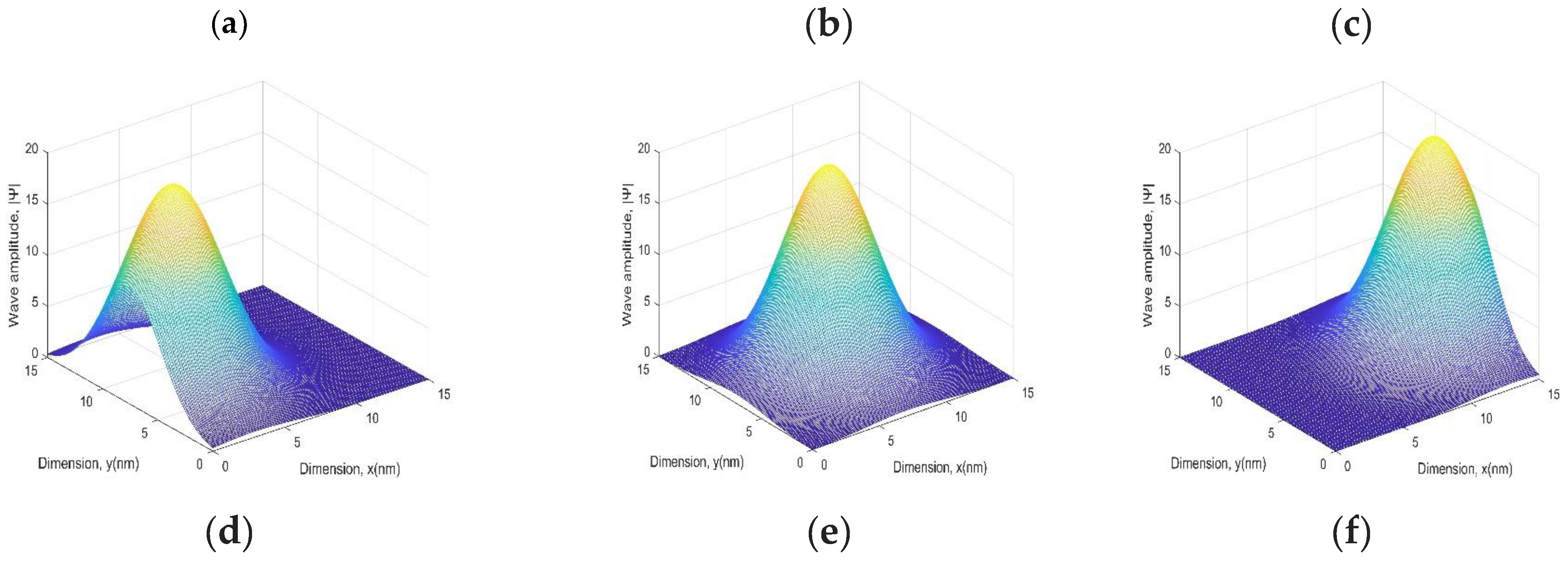
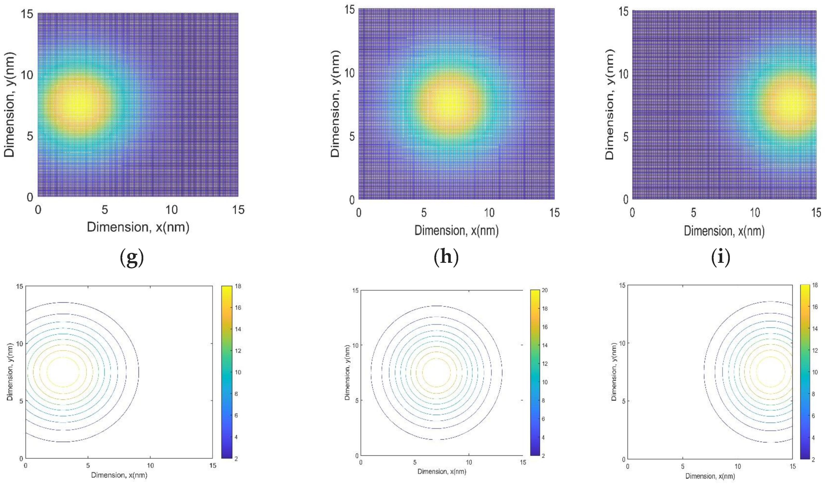
3.1.2. Results and Discussion

The obtained simulations of the 2D bright soliton presented in the 2D and 3D plots of Figure 2 are in excellent agreement with the results exhibited in [18,19,20,21].
Moreover, as inferred by the preceding numerical findings presented specifically in Table 1 and Table 2, the SSFT has demonstrated a superb performance over the other proposed methods. This is remarkably noted due to the least achieved SSE values in terms of 10 × 10 22 , which is almost zero, along with the smallest CPU processing time for manipulating this problem. This unique behavior might have occurred because of the employment of the splitting technique between the linear and nonlinear parts of the partial differential equation while solving them separately, in addition to the leverage of implementing the fast Fourier transform algorithm in this scheme [30,33,34]. Furthermore, it showed a perfect convergence due to exhibiting an absolute error in terms of 10 × 10 12 . This is shown in Figure 3a. The FPSM solution has remarkably consumed less CPU computational time when compared to the HSM, especially at high time values. In addition to this, the absolute error collapses whenever the temporal step size value diminishes, which substantiates its convergence as per Figure 3b. The HSM seems to be more meticulous than the FPSM. However, it is a time-consuming approach for solving the NLSE in two dimensions. Therefore, this method has been deduced to be more compatible with small-time values over a wide range of spatial values or further higher temporal values over a short range of spatial values. Its convergence is also numerically proved in Figure 3c.

3.2. Simulations of the 2D TDSE

In this section, to ascertain the effectiveness and accuracy of our proposed numerical schemes in solving the 2D TDSE, presented in Equation (22), copious numerical assessments have been performed. In this regard, we have utilized an initial Gaussian wave of the form [22,23,24,26]:
Ψ 0 x , y = 20 e i B x + C y e x M 2 + y H 2 ) 2 σ 2
where B   and C   are the propagation constants of the fundamental mode, M   and H   constitute the central position of the pulse at t = 0 . While σ indicates the spread of the pulse in the propagation direction. Furthermore, for simplicity, we have assumed that ξ and   η are equal to the unity in Equation (22).
For the validation purpose, a 3D graph of the absolute value of the analytical solution, presented in Equation (23), of the 2D TDSE is exhibited in Figure 4, where the exact solution is selected to be a Gaussian pulse over a domain of [0, 30] × [0, 30], computed at time t = 15 , while setting B and C to unity, σ to 2 2 , and M and H to 0 and 7, respectively.
Our experiments began by changing the physical domain into Ω= [0, 15] × [0, 15], which is discretized with a grid that is composed of 1 51 × 151 points, under a temporal step size of Δ t = 10 3 and spatial step sizes of Δ x = Δ y = 10 1 . Thereafter, we have plotted the numerical approximate solution of the 2D TDSE, within a period from t = 3   to 13, to mimic the electron’s wave motion while propagating through the quantum wire in two-dimension and three-dimension graphs, and further indicate the direction of the motion within the suggested period. As demonstrated in Figure 5, the SSFT approach was employed to simulate the absolute value of the electron wave function in (a, b, c) 3D graphs, (d, e, f) 2D graphs, and (g, h, i) contour plots at (a, d, g) t = 3 , (b, e, h) t = 7 , (c, f, i) t = 13 . To reach these specific times, “MATLAB R2021a” (The MathWorks, Inc., Natick, Massachusetts, United States) software has generated consecutive iterations of 3001, 7001, and 13,001, respectively.
The second part of this assessment aims to authenticate the accuracy and efficacy of the three suggested numerical schemes, which are the SSFT, FPSM, and HSM. In this regard, first, numerous experiments are established by employing an x and y domain of Ω = [0, 20] × [0, 20], which constructs a grid of 101 × 101 points, at a temporal step size of Δ t = 10 3 and spatial step sizes of Δ x   = Δ y = 2 × 10 1 . The modulus of the wave amplitudes has been computed abreast of their CPU elapsed time, using the three proposed approaches along with the analytical solution, at a specific time t = 6 , while seeking random x and y values within our predefined domain Ω, as represented in Table 3.

3.2.1. Error and Convergence Analysis

Thereafter, another experiment has performed over the same domain of Ω = [0, 20] × [0, 20], targeting higher time values within a range from t = 1 ,   15 , at a temporal step size of Δ t = 10 3 and spatial step sizes of Δ x = Δ y = 2 × 10 1 . This equally spaced domain has created a grid of 101 × 101 points, as mentioned earlier. Moreover, reaching time t = 10   has generated subsequent iterations of 10,001 while seeking a higher time t = 15   has produced more iterations of 15,001. Therefore, the MATLAB CPU processing time has been tracked as well in this assessment. In Table 4, a systematic comparison of the three proposed approaches is conducted to evaluate the SSE at different time values within our predefined domain Ω.
Eventually, for the convergence investigation of our proposed numerical schemes in reporting the 2D TDSE, three graphs have been implemented in Figure 6, as similarly followed in Figure 3 for the 2D NLSE, which demonstrate the relationship between a period of different temporal step sizes versus the absolute error. In Figure 6a, the SSFT was employed over a square domain of [0, 15] × [0, 15] while changing the temporal step size over a range from 0.0005 to 0.0095. This experiment was performed at consecutive times t = 10, 15,and 20. The same values were used for the FPSM and HSM, as shown in Figure 6b,c.

3.2.2. Results and Discussion

As substantiated in the previous section pertaining to the 2D NLSE, the graphical findings depicting the simulation of the 2D Gaussian wave through the quantum wire, demonstrated in Figure 5, using the SSFT are compatible with the results published in [22,23,24] using other methodologies.
Furthermore, the obtained numerical results listed in Table 3 and Table 4 endorsed that the SSFT renders the utmost feasible results, which are represented in establishing the highest accuracy level while consuming the least possible elapsed time. Therefore, it is perfectly compatible with the short and broad domains of the spatial and temporal values. As shown in Figure 6a, its absolute error is almost zero over different temporal step sizes, which corroborates its optimum convergence behavior.
The FPSM is a faster approach than the HSM. Hence, it is more reasonable for reaching higher temporal and spatial values. This scheme’s convergence is also numerically proven in Figure 6b as the error value drops down whenever the temporal step size decreases.
The HSM provides more accuracy than the FPSM. However, it is not desirable for high temporal values over broad spatial domains due to its slow-going behavior. Figure 6c declares the convergence of this scheme as well.
To sum up, the three suggested schemes are straightforward, rapid, effectual, and accurate for solving both the 2D NLSE and 2D TDSE. However, the SSFT is more efficient than the others in terms of speed, efficacy, and convergence.

4. Conclusions

In the PDE realm, analytical solutions are only known for a few scenarios. Therefore, numerical techniques are commonly used as an asset to explore the characteristics of their solutions. In this study, we presented three powerful approximate finite difference/pseudo-spectral techniques to solve the crucial 2D NLSE alongside the 2D TDSE; these techniques are called the SSFT, FPSM, and HSM. The 2D NLSE, which is a fundamental equation in nonlinear optics, was associated with a bright 1-soliton solution while a Gaussian wave solution was considered for the 2D TDSE, which is an eminent equation in quantum mechanics. The mathematical analysis was derived in this literature and corroborated by MATLAB simulations. The obtained numerical results of our proposed schemes were compared to the exact analytical solution to bolster their efficacy and credibility. Their outcomes were presented in either illustrative graphs or tables. Moreover, the analysis of the error and convergence were numerically computed. As a result, the MATLAB numerical findings elaborated that SSFT has exhibited a top-notch capability in the presented 2D simulations while sustaining the least possible execution time. Moreover, the FPSM has demonstrated a credible second-rank performance in terms of the consumed elapsed time. On the contrary, the HSM has been preferable over the short temporal and spatial domains that require less computational procedures due to its higher processing time. To recapitulate, the three suggested schemes are deemed to be dependable, robust, and effective for this simulation, hence they might be advantageous for approximating other types of equations in our future work.

Author Contributions

Conceptualization, S.S.A.O.; Investigation, N.G.A.F. and S.S.A.O.; Methodology, N.G.A.F.; Project administration, S.S.A.O.; Resources, N.G.A.F.; Software, N.G.A.F.; Supervision, A.H.E., M.S.E.-A. and S.S.A.O.; Validation, N.G.A.F.; Writing—original draft, N.G.A.F.; Writing—review & editing, N.G.A.F., A.H.E., M.S.E.-A. and S.S.A.O. All authors have read and agreed to the published version of the manuscript.

Funding

This research was accomplished as a part of the authors’ employment at their respected institutions. Therefore, no specific funding was received for the work presented in this paper.

Institutional Review Board Statement

Not applicable.

Informed Consent Statement

Not applicable.

Data Availability Statement

All relevant data are available upon request from the authors.

Conflicts of Interest

The authors declare that they have no potential conflict of interest.

References

  1. Jiwari, R.; Kumar, S.; Mittal, R.C.; Awrejcewicz, J. A meshfree approach for analysis and computational modeling of non-linear Schrödinger equation. Comput. Appl. Math. 2020, 39, 95. [Google Scholar] [CrossRef]
  2. Taha, T.R.; Ablowitz, M.I. Analytical and numerical aspects of certain nonlinear evolution equations. II. Numerical, nonlinear Schrödinger equation. J. Comput. Phys. 1984, 55, 203–230. [Google Scholar] [CrossRef]
  3. Akhmediev, N.N.; Korneev, V.I. Modulation Instability and Periodic Solutions of the Nonlinear Schrödinger Equation. Theor. Math. Phys. 1987, 69, 1089–1093. [Google Scholar] [CrossRef]
  4. Kibler, B.; Fatome, J.; Finot, C.; Millot, G.; Genty, G.; Wetzel, B.; Akhmediev, N.; Dias, F.; Dudley, J.M. Observation of Kuznetsov-Ma soliton dynamics in optical fibre. Sci. Rep. 2012, 2, 463. [Google Scholar] [CrossRef]
  5. Peregrine, D.H. Water waves, nonlinear Schrödinger equations and their solutions. ANZIAM J. 1983, 25, 16–43. [Google Scholar] [CrossRef]
  6. Kibler, B.; Fatome, J.; Finot, C.; Millot, G.; Dias, F.; Genty, G.; Akhmediev, N.; Dudley, J.M. The Peregrine soliton in nonlinear fibre optics. Nat. Phys. 2010, 6, 790–795. [Google Scholar] [CrossRef]
  7. Belić, M.R.; Nikolić, S.N.; Ashour, O.A.; Aleksić, N.B. On different aspects of the optical rogue waves nature. Nonlinear Dyn. 2022, 108, 1655–1670. [Google Scholar] [CrossRef]
  8. Akhmediev, N.; Kibler, B.; Baronio, F.; Belić, M.; Zhong, W.P.; Zhang, Y.; Chang, W.; Soto-Crespo, J.M.; Vouzas, P.; Grelu, P.; et al. Roadmap on optical rogue waves and extreme events. J. Opt. 2016, 18, 063001. [Google Scholar] [CrossRef]
  9. Nikolić, S.N.; Radonjić, M.; Lučić, N.M.; Krmpot, A.J.; Jelenković, B.M. Transient development of Zeeman electromagnetically induced transparency during propagation of Raman-Ramsey pulses through Rb buffer gas cell. J. Phys. B At. Mol. Opt. Phys. 2015, 48, 045501. [Google Scholar] [CrossRef]
  10. Li, Z.Y.; Li, F.F.; Li, H.J. Exciting rogue waves, breathers, and solitons in coherent atomic media. Commun. Theor. Phys. 2020, 72, 075003. [Google Scholar] [CrossRef]
  11. Hu, H.; Chen, Y. Numerical solution of two-dimensional nonlinear Schrödinger equation using a new two-grid finite element method. J. Comput. Appl. Math. 2020, 364, 112333. [Google Scholar] [CrossRef]
  12. Sun, Z. A conservative scheme for two-dimensional Schrödinger equation based on multiquadric trigonometric quasi-interpolation approach. Appl. Math. Comput. 2022, 423, 126996. [Google Scholar] [CrossRef]
  13. Antoine, X.; Besse, C.; Klein, P.; Antoine, X.; Besse, C.; Klein, P.; Solution, N. Nonlinear, Numerical Solution of Time-Dependent Nonlinear Schrödinger Equations Using Domain Truncation Techniques Coupled with Relaxation Scheme. Laser Phys. 2011, 21, 1491–1502. [Google Scholar] [CrossRef]
  14. Wang, Y.; Hao, Z.; Du, R. A Linear Finite Difference Scheme for the Two-Dimensional Nonlinear Schrödinger Equation with Fractional Laplacian. J. Sci. Comput. 2022, 90, 24. [Google Scholar] [CrossRef]
  15. Geng, J.; Xue, S. Reducible KAM tori for two-dimensional nonlinear Schrödinger equations with explicit dependence on the spatial variable. J. Funct. Anal. 2022, 282, 109430. [Google Scholar] [CrossRef]
  16. Seadawy, A.R. Exact solutions of a two-dimensional nonlinear Schrödinger equation. Appl. Math. Lett. 2012, 25, 687–691. [Google Scholar] [CrossRef]
  17. Bulut, H.; Pandir, Y.; Tuluce, S. Demiray, Exact solutions of nonlinear Schrödingers equation with dual power-law nonlinearity by extended trial equation method. Waves Random Complex Media 2014, 24, 439–451. [Google Scholar] [CrossRef]
  18. Durur, H.; Ilhan, E.; Bulut, H. Novel complex wave solutions of the (2+1)-dimensional hyperbolic nonlinear schrödinger equation. Fractal Fract. 2020, 4, 41. [Google Scholar] [CrossRef]
  19. Wang, L.; Luan, Z.; Zhou, Q.; Biswas, A.; Alzahrani, A.; Liu, W. Bright soliton solutions of the (2+1)-dimensional generalized coupled nonlinear Schrödinger equation with the four-wave mixing term. Nonlinear Dyn. 2021, 104, 2613–2620. [Google Scholar] [CrossRef]
  20. Burdik, C.; Shaikhova, G.; Rakhimzhanov, B. Soliton solutions and traveling wave solutions of the two-dimensional generalized nonlinear Schrödinger equations. Eur. Phys. J. Plus. 2021, 136, 1095. [Google Scholar] [CrossRef]
  21. Moxley, F.I.; Chuss, D.T.; Dai, W. A generalized finite-difference time-domain scheme for solving nonlinear Schrödinger equations. Comput. Phys. Commun. 2013, 184, 1834–1841. [Google Scholar] [CrossRef]
  22. Kalita, J.C.; Chhabra, P.; Kumar, S. A semi-discrete higher order compact scheme for the unsteady two-dimensional Schrödinger equation. J. Comput. Appl. Math. 2006, 197, 141–149. [Google Scholar] [CrossRef]
  23. Dehghan, M.; Shokri, A. A numerical method for two-dimensional Schrödinger equation using collocation and radial basis functions. Comput. Math. Appl. 2007, 54, 136–146. [Google Scholar] [CrossRef]
  24. Jin, J.; Wu, X. Convergence of a finite element scheme for the two-dimensional time-dependent Schrödinger equation in a long strip. J. Comput. Appl. Math. 2010, 234, 777–793. [Google Scholar] [CrossRef]
  25. Tian, Z.; Chen, Y.; Huang, Y.; Wang, J. Two-grid method for the two-dimensional time-dependent Schrödinger equation by the finite element method. Comput. Math. Appl. 2019, 77, 3043–3053. [Google Scholar] [CrossRef]
  26. Gotoh, H.; Koshiba, M.; Tsuji, Y. Finite-element time-domain beam propagation method with perfectly matched layer for electron waveguide simulations. IEICE Electron. Express 2011, 8, 1361–1366. [Google Scholar] [CrossRef]
  27. Atia, K.S.R.; Heikal, A.M.; Obayya, S.S.A. Smoothed finite element method for time dependent analysis of quantum resonance devices. Opt. Quantum Electron. 2018, 50, 127. [Google Scholar] [CrossRef]
  28. Khordad, R.; Firoozi, A.; Sedehi, H.R.R. Simultaneous Effects of Temperature and Pressure on the Entropy and the Specific Heat of a Three-Dimensional Quantum Wire: Tsallis Formalism. J. Low Temp. Phys. 2021, 202, 185–195. [Google Scholar] [CrossRef]
  29. Jiang, T.; Chen, Z.C.; Lu, W.G.; Yuan, J.Y.; Wang, D.S. Efficient split-step and implicit pure mesh-free method for the 2D/3D nonlinear Gross–Pitaevskii equations. Comput. Phys. Commun. 2018, 231, 19–30. [Google Scholar] [CrossRef]
  30. Farag, N.G.; Eltanboly, A.H.; El-Azab, M.S.; Obayya, S.S.A. Pseudo-spectral approach for extracting optical solitons of the complex Ginzburg Landau equation with six nonlinearity forms. Optik 2022, 254, 168662. [Google Scholar] [CrossRef]
  31. Zheng, R.; Liu, F.; Jiang, X.; Turner, I.W. Finite difference/spectral methods for the two-dimensional distributed-order time-fractional cable equation. Comput. Math. Appl. 2020, 80, 1523–1537. [Google Scholar] [CrossRef]
  32. Han, C.; Wang, Y.L. Numerical Solutions of Variable-Coefficient Fractional-in-Space KdV Equation with the Caputo Fractional Derivative. Fractal Fract. 2022, 6, 207. [Google Scholar] [CrossRef]
  33. Farag, N.G.; Eltanboly, A.H.; El-Azab, M.S.; Obayya, S.S.A. On the Analytical and Numerical Solutions of the One-Dimensional Nonlinear Schrödinger Equation. Math. Probl. Eng. 2021, 2021, 3094011. [Google Scholar] [CrossRef]
  34. Farag, N.G.; Eltanboly, A.H.; El-Azab, M.S.; Obayya, S.S.A. Extended Split-Step Fourier Transform Approach for Accurate Characterization of Soliton Propagation in a Lossy Optical Fiber. J. Funct. Spaces 2022, 2022, 8316404. [Google Scholar] [CrossRef]
  35. Alshammari, F.S.; Akyildiz, F.T. Pseudo spectral solution of extended Graetz problem for combined pressure-driven and electroosmotic flow in a triangular micro-duct. Comput. Math. Appl. 2020, 80, 990–1008. [Google Scholar] [CrossRef]
  36. Vajta, M. Approximate solution of a nonlinear partial differential equation. In Proceedings of the 2007 Mediterranean Conference on Control & Automation, Athens, Greece, 27–29 June 2007. [Google Scholar] [CrossRef]
  37. Wazwaz, A.M.; Alhejaili, W.; El-Tantawy, S.A. Bright and dark envelope optical solitons for a (2+1)-dimensional cubic nonlinear Schrödinger equation. Optik 2022, 265, 169525. [Google Scholar] [CrossRef]
  38. Suarez, P.; Su, P.U. An introduction to the Split Step Fourier Method using MATLAB. ResearchGate 2016. [Google Scholar] [CrossRef]
Figure 1. Exact solution of the 2D NLSE with a bright soliton input pulse, at time t = 10 , over x and y domains of [−20, 20] × [−20, 20].
Fractalfract 07 00188 g001
Figure 2. (ac) Three-dimensional graphs, (df) 2D graphs, and (gi) contour plots for simulating the free-space propagation of the 2D bright soliton, using the SSFT for solving the 2D NLSE with Δ t = 10 3 and Δ x = Δ y = 2 × 10 1 , at different times (a,d,g) t = 1 , (b,e,h) t = 3 , (c,f,i) t = 6 , over x and y domains of [−30, 30] × [−30, 30].
Fractalfract 07 00188 g002aFractalfract 07 00188 g002b
Figure 3. Comparative graphs representing the relationship between a range of different temporal step sizes, when Δ x = Δ y = 2 × 10 1 , versus the obtained absolute error, using (a) the SSFT, (b) the FPSM, for solving the 2D NLSE, at different times t = 3 , t = 5 , and t = 7 , over x and y domains of [−20, 20] × [−20, 20], whereas using different time values of t = 1 , t = 1.5 , and t = 2 , over x and y domains of [−10, 10] × [−10, 10] for (c) the HSM.
Fractalfract 07 00188 g003
Figure 4. Exact solution of the 2D TDSE simulating the propagation of the Gaussian input pulse, at time t = 15 , over x and y domains of [0, 30] × [0, 30].
Fractalfract 07 00188 g004
Figure 5. (ac) Three-dimensional graphs, (df) 2D graphs, and (gi) contour plots for simulating the propagation of the 2D Gaussian pulse through the quantum wire in the z-direction, using the SSFT for solving the 2D TDSE with Δ t = 10 3 and Δ x = Δ y = 10 1 , at different times (a,d,g) t = 3 , (b,e,h) t = 7 , (c,f,i) t = 13 , over x and y domains of [0, 15] × [0, 15].
Fractalfract 07 00188 g005aFractalfract 07 00188 g005b
Figure 6. Comparative graphs representing the relationship between a range of different temporal step sizes, when Δ x = Δ y = 2 × 10 1 , versus the obtained absolute error, using (a) the SSFT, (b) the FPSM, (c) the HSM, for solving the 2D TDSE, at different times t = 10 , t = 15 , and t = 20 over x and y domains of [0, 15] × [0, 15].
Fractalfract 07 00188 g006
Table 1. A comparison of the modulus of the wave amplitude at time t = 1 and different x and y values, using the SSFT, FPSM, and HSM, at Δ x = Δ y = 2 × 10 1 and Δ t = 10 3 , and the exact analytical solution, over x and y domains of [−20, 20] × [−20, 20] for the 2D NLSE.
x y | Ψ | -SSFT | Ψ | -FPSM | Ψ | -HSM | Ψ | -EXACT CPU Time(s)-SSFT CPU Time(s)-FPSM CPU Time(s)-HSM
1 5 1.9057 × 10 2 2.0523 × 10 2 1.9095 × 10 2 1.9057 × 10 2 2.5108 3.6608 1.0901 × 10
2 7 9.4883 × 10 4 1.0218 × 10 3 9.5074 × 10 4 9.4883 × 10 4 2.250 3.5893 1.0856 × 10
3 8 1.2841 × 10 4 1.3829 × 10 4 1.2867 × 10 4 1.2841 × 10 4 2.1515 3.9462 1.2564 × 10
5 10 2.3519 × 10 6 2.5329 × 10 6 2.3567 × 10 6 2.3519 × 10 6 2.1435 4.9033 1.0614 × 10
7 13 1.5847 × 10 8 1.7066 × 10 8 1.5879 × 10 8 1.5847 × 10 8 2.1152 3.8490 1.0929 × 10
9 14 7.8905 × 10 10 8.4968 × 10 10 7.9057 × 10 10 7.8898 × 10 10 2.138 3.5086 1.0966 × 10
10 15 1.0680 × 10 10 1.1499 × 10 10 1.0699 × 10 10 1.0678 × 10 10 2.1300 3.4625 1.1075 × 10
Table 2. A comparison of the sum of squares error (SSE) of the SSFT, FPSM, and HSM, at Δ x = Δ y = 2 × 10 1 and Δ t = 10 3 , and the exact analytical solution along with the CPU processing time at different time values t   [0.1, 2], over x and y domains of [−20, 20] × [−20, 20] for the 2D NLSE.
Time, tSSFT-SSEFPSM-SSEHSM-SSECPU Time(s)-SSFTCPU Time(s)-FPSMCPU Time(s)-HSM
0.1 1.1245 × 10 23 1.3906 × 10 1 1.3824 × 10 1 3.3838 × 10 1 5.2151 × 10 1 1.6471
0.2 4.3874 × 10 23 5.5797 × 10 1 3.5031 × 10 1 4.6749 × 10 1 7.9404 × 10 1 3.2275
0.4 1.6982 × 10 22 2.2446 8.6132 × 10 1 8.7677 × 10 1 1.4244 5.6874
0.5 2.6874 × 10 22 3.5160 1.1819 1.1225 1.7936 7.4073
1 1.0716 × 10 21 1.4204 × 10 9.3939 2.1427 3.4773 1.4721 × 10
1.5 2.4222 × 10 21 3.2157 × 10 1.3036 × 10 2 3.4239 5.3946 2.1097 × 10
2 4.2536 × 10 21 5.7390 × 10 5.7535 × 10 2 4.2984 7.1198 2.7243 × 10
Table 3. A comparison of the modulus of the wave amplitude alongside the execution time, at time t = 6   and different x and y values, using the SSFT, FPSM, and HSM solutions, at Δ x = Δ y = 2 × 10 1   Δ t = 10 3 , over x and y domains of [0, 20] × [0, 20] for the 2D TDSE.
xy | Ψ | -SSFT | Ψ | -FPSM | Ψ | -HSM | Ψ | -Exact CPU Time-SSFT (s)CPU Time-FPSM (s)CPU Time-HSM (s)
12 3.3481 × 10 2 5.6360 × 10 2 3.3671 × 10 2 3.3481 × 10 2 9.7617 1.7982 × 10 2.0319 × 10
33 4.1302 × 10 1 6.9525 × 10 1 4.1317 × 10 1 4.1302 × 10 1 9.7447 1.8179 × 10 2.0544 × 10
491.10871.86641.10881.10879.9013 1.7964 × 10 2.0502 × 10
6102.69324.53362.69722.69329.7623 1.8005 × 10 2.0722 × 10
8121.80533.03901.81181.80539.7739 1.8002 × 10 2.0316 × 10
9131.01591.71001.02031.01599.7287 1.8012 × 10 2.1132 × 10
1015 1.5775 × 10 1 2.6554 × 10 1 1.5848 × 10 1 1.5775 × 10 1 9.7627 1.8001 × 10 2.4169 × 10
Table 4. A comparison of the sum of squares error (SSE) of the SSFT, FPSM, and HSM, at Δ x = Δ y = 2 × 10 3   and Δ t = 10 1 , and the exact analytical solution along with the CPU processing time at different time values t   [1, 15], over x and y domains of [0, 20] × [0, 20] for the 2D TDSE.
Time, tSSFT-SSEFPSM-SSEHSM-SSECPU Time(s)-SSFTCPU Time(s)-FPSMCPU Time(s)-HSM
1 2.4098 × 10 23 2.1779 × 10 4 2.6489 × 10 2 1.69613.35413.4406
3 2.8561 × 10 22 3.1057 × 10 3 3.5105 × 10 2 4.94919.0329 1.0188 × 10
6 9.6769 × 10 22 1.7428 × 10 2 3.7323 × 10 2 9.8193 1.7994 × 10 2.0811 × 10
8 2.1952 × 10 21 3.7548 × 10 2 3.7364 × 10 2 1.2958 × 10 2.3946 × 10 2.8573 × 10
10 2.9793 × 10 21 7.1372 × 10 2 3.7365 × 10 2 1.6463 × 10 2.9894 × 10 3.8181 × 10
12 5.2078 × 10 21 1.2563 × 10 1 3.7364 × 10 2 1.9430 × 10 3.5876 × 10 5.3228 × 10
15 5.3166 × 10 21 2.6623 × 10 1 3.7165 × 10 2 2.4539 × 10 4.8238 × 10 5.9862 × 10
Disclaimer/Publisher’s Note: The statements, opinions and data contained in all publications are solely those of the individual author(s) and contributor(s) and not of MDPI and/or the editor(s). MDPI and/or the editor(s) disclaim responsibility for any injury to people or property resulting from any ideas, methods, instructions or products referred to in the content.

