Article

Analytical Computational Scheme for Multivariate Nonlinear Time-Fractional Generalized Biological Population Model

1
Department of Mathematics, Faculty of Arts and Science, Amman Arab University, Amman 11953, Jordan
2
Department of Mathematics, Faculty of Science, Yarmouk University, Irbid 22163, Jordan
3
Department of Mathematics, Faculty of Science, The Hashemite University, P.O. Box 330127, Zarqa 13133, Jordan
4
Department of Mathematical Sciences, Faculty of Science and Technology, Universiti Kebangsaan Malaysia (UKM), Bangi 43600, Malaysia
*
Author to whom correspondence should be addressed.
Fractal Fract. 2023, 7(2), 176; https://doi.org/10.3390/fractalfract7020176
Submission received: 19 December 2022 / Revised: 19 January 2023 / Accepted: 7 February 2023 / Published: 10 February 2023

Abstract

:
This work provides exact and analytical approximate solutions for a non-linear time-fractional generalized biology population model (FGBPM) with suitable initial data under the time-Caputo fractional derivative, in view of a novel effective and applicable scheme, based upon elegant amalgamation between the Laplace transform operator and the generalized power series method. The solution form obtained by the proposed algorithm of considered FGBPM is an infinite multivariable convergent series toward the exact solutions for the integer fractional order. Some applications of the posed model are tested to confirm the theoretical aspects and highlight the superiority of the proposed scheme in predicting the analytical approximate solutions in closed forms compared to other existing analytical methods. Associated figure representations and the results are displayed in different dimensional graphs. Numerical analyses are performed, and discussions regarding the errors and the convergence of the scheme are presented. The simulations and results report that the proposed modern scheme is, indeed, direct, applicable, and effective to deal with a wide range of non-linear time multivariable fractional models.

1. Introduction

In the past few years, the topic of fractional calculus (FC), including differentiation and integration of non-integer order, is being employed comprehensively in various scientific sectors and is growing uncommonly vast in the evolution of novel models because of its connection with memory and fractal kinds which are profuse in physical phenomena [1,2,3,4]. The beauty of FC is in incorporating fractional-order derivatives into the considered model reduces inaccuracy caused by unawareness of the parameters for the model structure. Moreover, it allows for a better degree of freedom in models of physical phenomena compared with ordinary systems. Recently, numerous models in dynamics and biology [5,6,7] have been modeled with the help of fractional-order derivatives which express the behavior of real-life phenomena suitably and applicably. Fractional differential equations (FDEs) are armed with magnificent approaches for describing hereditary and memory features which are disregarded by ordinary systems.
Non-linear fractional and ordinary differential equations play a prime role in diverse scopes such as biology, physics, engineering, and fluid mechanics. Obtaining analytical solutions to these problems is not always possible [8,9,10,11,12,13,14]. Thereby, it is considerable to handle these problems appropriately and solve them or develop solutions. In this orientation, many researchers have proposed and employed several analytical and numerical techniques, including the variational iteration method (VIM) [15,16], fractional wavelet method (FWM) [17], homotopy analysis method (HAM) [18,19], and fractional power series method (FPSM) [20,21,22,23].
The main theme work is to analyze and provide the exact and analytical approximate solutions for the time non-linear biological population model with time-fractional Caputo-derivative. To this end, we consider the time non-linear fractional biological population model (FBPM) form as follows:
D t α ω η , t = D x 2 ω 2 η , t + D y 2 ω 2 η , t + F ω , α 0,1 , t 0 ,
with initial condition ω η , 0 = ρ 0 η , where D t α is the α -th time-fractional Caputo-derivative, and ω η , t is the population density, which is defined by the three parameters, the positions η = ( x , y ) , and the time t , and provides the individual number per unit volume. While F ω represents the population supply due to births and deaths. When α 1 , various merits of FGBPM (1), such as Hölder estimates of its solutions, are studied in [24]. The population supply function F ω has the following constitutive cases:
  • If F ω = k ω , then FBPM (1) reduces to Malthusian law [25] and k constant;
  • If F ω = k ω - l ω 2 , then FBPM (1) reduces to Verhulst law [24] and k , l positive constants;
  • If F ω = k ω ϑ , then FBPM (1) reduces to porous media [26], k positive constants, and ϑ ( 0,1 ) .
More specifically, we consider and discuss the more general form of F in (1) as F ω = λ ω p 1 - r ω q , where λ , r , p , and q are real numbers. Thus, the time non-linear FBPM is extended to the following time non-linear generalized FBPM (FGBPM):
D t α ω η , t = D x 2 ω 2 η , t + D y 2 ω 2 η , t + λ ω p 1 - r ω q , α 0,1 , t 0 ,
Various numeric–analytic methods have been applied to solve the time non-linear FBPM (1) and FGBPM (2) with numerous fractional derivatives [27,28,29,30]. In this article, a novel solution scheme is proposed to gain the exact and analytical approximate solutions using the methodology of Laplace FPSM [31,32]. It is a superb amalgamation of Laplace transform (LT) and FPSM to treat several non-linear fractional models arising in physics and engineering fields, including the time-fractional Broer–Kaup–Burger model [33], time-fractional Kolmogorov and Rosenau–Hyman models [34], temporal time-fractional gas dynamics models [35], and complex fuzzy fractional population dynamics models [36]. The recommended method produces the analytical approximate solutions in the fast convergent form of the fractional series expansion after solving the considered model in Laplace space via employing the residual error concept and utilizing the limit concept with no required restrictive assumptions and reduces mathematical calculations notably. Thus, what characterizes the Laplace FPSM is solving the target fractional model in the Laplace space, making it easier than solving it with the original space and considering the concept of the limit at infinity when finding the proposed expansion coefficients, and replacing the fractional derivation stage, as is the case in FPSM [37,38]. Consequently, the superiority of the novel solution approach appears in its capability to generate closed-form and accurate approximate solutions. Hereinafter, some fundamental definitions and primary results concerning the FC topic and Laplace multivariate FS representations have been reported briefly. In Section 3, a basic methodology of multivariate Laplace FPSM is designed and clarified for solving nonlinear time FGBPM (2). In Section 4, the applicability and performance of the proposed scheme are achieved by performing it on attractive applications of the posed model. Lastly, some concluding remarks on our findings are drawn.

2. Preliminary Mathematical Concepts

This segment is aimed to highlight the basic definitions and some preliminary results of FC theory with its features. Furthermore, a revisiting of the multivariate Laplace FPSM in the Caputo fractional derivative sense is undertaken.
Definition 1. 
The α -th time fractional Riemann–Liouville integral operator of multivariable ω C δ , δ - 1 , denoted by J t α and given by [2]:
J t α ω η , t = 1 Γ ( α ) 0 t ω η , ϑ ( t - ϑ ) 1 - α d ϑ , α n - 1 , n , n N , J t 0 ω η , t = ω η , t .
Definition 2 
([2]). The α -th time fractional derivative in the Caputo sense of multivariable ω C δ , δ - 1 , denoted by D t α and given by:
D t α ω η , t = n x n ω ( η , t ) , α = 0 J t n - α n η n ω ( η , t ) , α n - 1 , n , n N ,
Definition 3 
([31]). Assume that ω η , t : R 2 × [ 0 , ) R . The LT of ω ( η , t ) is defined as:
W η , ξ = L ω η , t = 0 + ω η , t e - ξ t d t , ξ > ρ ,
and the inverse LT of the new function W η , ξ is defined as:
ω x , t = L - 1 W η , ξ = ϵ - i ϵ + i W η , ξ e ξ t d ξ , ϵ = R e ( ξ ) > ϵ 0 ,
with the following characteristics:
  • L t m α = Γ m α + 1 ξ m α + 1 ,   α > - 1 .
  • lim ξ + ξ W η , ξ = ω η , 0 .
  • L a ω η , t + b z η , t = a W η , ξ + b Z η , ξ , for any a , b R .
  • L - 1 a W η , ξ + b Z η , ξ = a ω η , t + b z η , t .
where W η , ξ = L ω η , t , and Z η , ξ = L z η , t .
Lemma 1. 
Suppose that ω η , t : R 2 × [ 0 , ) R and the exponential order. Then,
i. L D t α ω η , t = ξ α W η , ξ - k = 0 n - 1 ξ α - k - 1 ω t ( k ) η , 0 , α ( n - 1 , n ] , n N .
ii. L D t m α ω η , t = ξ m α W η , ξ - k = 0 m - 1 ξ ( m - k ) α - 1 D t k α ω η , 0 , α ( 0,1 ] , m N .
Theorem 1 
([31]). Suppose that ω η , t
is a continuous multivariable function on R 2 × [ 0 , + ) , then the transform function W η , ξ could be expressed in the following Laplace fractional expansion (FE):
W η , ξ = n = 0 ω n ( η ) ξ n α + 1 , ξ > 0 , α 0 , 1 ,
where the coefficients ω n ( η ) = D t n α ω n ( η ) .
Remark 1. 
The inverse LT of the Laplace FE (7) has the following fractional series solution (FSS):
ω η , t = n = 0 D t n α ω n ( η ) Γ n α + 1 t n α , t 0 , α 0 , 1 ,
where ω η , t is infinitely the time-fractional derivative in Caputo sense at any point t ( 0 , r 1 α ] .
Theorem 2 
([31]). Let ξ L D t ( n + 1 ) α ω η , t l η , on R m × δ , γ where 0 < α 1 . Then, the remainder of the fractional series solution (FSS)(8) satisfies the following inequality:
R n η , ξ l η l 1 + n + 1 α , η R m , δ < ξ γ .

3. Principle of the Laplace FPSM

The Laplace FPSM is an analytical computational scheme that has been suggested, particularly in [31], to handle emerging time-fractional PDEs in various nonlinear dynamical phenomena. The proposed scheme is a promotion of FPSM with an LT operator. It is based on solving the studied model in the Laplace space using the simulation FPSM in obtaining the expansion unknown functions via a new procedure easier than the traditional FPSM. In this segment, a novel algorithm is designed and developed for generating the analytical approximate FSS of the nonlinear time-FGBPM (2) with initial conditions in a specific space–time domain. To reach our main theme, we convert (2) into the Laplace space, and using Lemma 1 part (ii), we have:
W x , y , ξ = ω 0 ( x , y ) ξ + 1 ξ α L L - 1 D x 2 W x , y , ξ 2 + 1 ξ α L L - 1 D y 2 W x , y , ξ 2 + λ ξ α L L - 1 W x , y , ξ p - λ r ξ α L L - 1 W x , y , ξ p + q .
The proposed solution of (10) has the Laplace FE series:
W x , y , ξ = n = 0 ω n ( x , y ) ξ n α + 1 , ξ > 0 , α 0 , 1 ,
provided that ω 0 x , y = ρ 0 ( x , y ) . Thus, the j -th truncated Laplace FE series W j x , y , ξ , could be expressed as:
W j x , y , ξ = ρ 0 x , y + n = 1 j ω n ( x , y ) ξ n α + 1 , ξ > 0 , α 0 , 1 ,
To find out the unknown function ω n x , y , we define the so-called Laplace–residual error function (L-REF) of (10) as:
L R e s W x , y , ξ = W x , y , ξ - ω 0 x , y ξ - 1 ξ α L L - 1 D x 2 W x , y , ξ 2 - 1 ξ α L L - 1 D y 2 W x , y , ξ 2 - λ ξ α L L - 1 W x , y , ξ p + λ r ξ α L L - 1 W x , y , ξ p + q .
Meanwhile, the j -th truncated the L-REF of (13) will be:
L R e s W j x , y , ξ = W j x , y , ξ - ω 0 x , y ξ - 1 ξ α L L - 1 D x 2 W j x , y , ξ 2 - 1 ξ α L L - 1 D y 2 W j x , y , ξ 2 - λ ξ α L L - 1 W j x , y , ξ p + λ r ξ α L L - 1 W j x , y , ξ p + q .
To explain the presence of the main idea of the proposed scheme in detecting the analytical approximate FSS of the considered model (2), the following underlying algorithm is dedicated:
Step I: Assume that the solution of the new Laplace Equation (10) has the Laplace FE series (12).
Step II: Define the j -th truncated Laplace FE series W j x , y , ξ , as in (13).
Step III: Define the j -th truncated L-REF L R e s W j x , y , ξ of (13), as given in (14).
Step IV: Substitute the j -th truncated Laplace FE series W j x , y , ξ obtained in Step II into L R e s W j x , y , ξ , obtained in Step III, as follows:
L R e s W j x , y , ξ = n = 1 j ω n ( x , y ) ξ n α + 1 - 1 ξ α L L - 1 D x 2 ρ 0 x , y + n = 1 j ω n ( x , y ) ξ n α + 1 2 - 1 ξ α L L - 1 D y 2 ρ 0 x , y + n = 1 j ω n ( x , y ) ξ n α + 1 2 - λ ξ α L L - 1 ρ 0 x , y + n = 1 j ω n ( x , y ) ξ n α + 1 p + λ r ξ α L L - 1 ρ 0 x , y + n = 1 j ω n ( x , y ) ξ n α + 1 p + q .
Step V: Multiply the obtained equation in Step IV by the factor ξ j α + 1 , and then solve the system lim ξ + ξ n α + 1 L R e s W j x , y , ξ for ω j ( x , y ) .
Step VI: Cumulate the unknown functions ω j ( x , y ) determined in Step V in terms of j -th truncated Laplace FE series W j x , y , ξ (12). When j , the Laplace FE series W x , y , ξ (11) can be obtained.
Step VII: Eventually, running the inverse LT to the obtained Laplace expansion in Step VI yields the analytical approximate FSS of the studied model (2).

4. Applications

In this section, the applicability of the Laplace FPSM is investigated to construct the analytical exact and approximate FSS of certain special cases of nonlinear time FGBPM (2) with suitable ICs. Further, simulations and graphical representations were investigated for the obtained results of the studied models. Symbolic and computations were performed using Mathematica 12.
Application 1. 
Consider the nonlinear time-FBPM given as:
D t α ω = D x 2 ω 2 + D y 2 ω 2 + λ ω , α 0,1 ,
According to the previous discussion, by first applying LT to Equation (15) with Lemma 1, part (ii), we obtain:
W x , y , ξ = ω 0 ( x , y ) ξ + 1 ξ α L L - 1 D x 2 W x , y , ξ 2 + 1 ξ α L L - 1 D y 2 W x , y , ξ 2 + λ ξ α W x , y , ξ .
Hence, the L-REF of (17) can be identified as:
L R e s W x , y , ξ = W x , y , ξ - ω 0 x , y ξ - 1 ξ α L L - 1 D x 2 W x , y , ξ 2 - 1 ξ α L L - 1 D y 2 W x , y , ξ 2 - λ ξ α W x , y , ξ .
Meanwhile, the j -th truncated L-REF can be expressed as:
L R e s W j x , y , ξ = W j x , y , ξ - ω 0 x , y ξ - 1 ξ α L L - 1 D x 2 W j x , y , ξ 2 - 1 ξ α L L - 1 D y 2 W j x , y , ξ 2 - λ ξ α W j x , y , ξ .
where the j -th transform function W j x , y , ξ takes the Laplace FE form:
W j x , y , ξ = m = 0 j ω m x , y ξ m α + 1   ξ > 0 ,
Now, to investigate the analytical solution to the main problem, we should find out the form of the unknown functions ω m x , y for m = 0,1 , 2 , . . j . To this end, we substitute the j -th transform function W j x , y , ξ (20) into the j -th truncated L-REF (19) such that:
L R e s W j x , y , ξ = m = 1 j ω m x , y ξ m α + 1 - 1 ξ α L L - 1 D x 2 m = 0 j ω m x , y ξ m α + 1 2 - 1 ξ α L L - 1 D y 2 m = 0 j ω m x , y ξ m α + 1 2 - λ ξ α m = 0 j ω m x , y ξ m α + 1 .
Multiply both sides of the obtained Equation (20) by the factor ξ m α + 1 , and we have:
ξ m α + 1 L R e s W j x , y , ξ = ω j x , y - λ ω j - 1 x , y - Γ ( j - 1 α + 1 ) ( i = 0 j - 1 2 D y ω i x , y D y ω j - i - 1 x , y + D y 2 ω i x , y ω - i + j - 1 x , y + ω i x , y D y 2 ω j - i - 1 x , y Γ i α + 1 Γ - i + j - 1 α + 1 + i = 0 j - 1 2 D x ω i x , y D x ω j - i - 1 x , y + D x 2 ω i x , y ω - i + j - 1 x , y + ω i x , y D x 2 ω j - i - 1 x , y Γ ( i α + 1 ) Γ ( ( - i + j - 1 ) α + 1 ) ) .
After that, we can solve (21) for ω j x , y to obtain the following recurrence relation:
ω j x , y = λ ω j - 1 x , y + Γ ( ( j - 1 ) α + 1 ) ( i = 0 j - 1 2 D y ω i x , y D y ω j - i - 1 x , y + D y 2 ω i x , y ω - i + j - 1 x , y + ω i x , y D y 2 ω j - i - 1 x , y Γ i α + 1 Γ - i + j - 1 α + 1 + i = 0 j - 1 2 D x ω i x , y D x ω j - i - 1 x , y + D x 2 ω i x , y ω - i + j - 1 x , y + ω i x , y D x 2 ω j - i - 1 x , y Γ ( i α + 1 ) Γ ( ( - i + j - 1 ) α + 1 ) ) .
Using Mathematica Software 12 and considering the initial condition ω 0 x , y = x y into (22), we can easily find out the forms of ω j x , y for j = 1,2 , . In this direction, more unknown functions could be computed.
ω 1 x , y = λ x y , ω 2 x , y = λ 2 x y , ω 3 x , y = λ 3 x y , ω j x , y = λ j x y .
So, by grouping the obtained ω j x , y in terms of expansion (19), we can predict the j -th Laplace FE of (16) in the form:
W j x , y , ξ = x y + λ x y ξ α + 1 + λ 2 x y ξ 2 α + 1 + + λ j x y ξ j α + 1 .
When j , the Laplace FE of (16) takes the form:
W x , y , ξ = x y 1 + λ ξ α + 1 + λ 2 ξ 2 α + 1 + + λ j ξ j α + 1 + = x y m = 0 λ m ξ m α + 1 .
As the last step in finding the analytical approximate FSS, we convert the fractional expansion (24) into the main space by performing the inverse LT on the result (24). Consequently, the analytical approximate FSS of the nonlinear time-FBPM (15) could be formulated in the following closed form:
ω x , y , t = x y m = 0 λ t α m Γ m α + 1 = x y E α λ t α .
Particularly, for α = 1 , the analytical approximate FSS (26) reduces to the exact solution:
ω x , y , t = x y m = 0 λ t m Γ m + 1 = x y e λ t ,
which meets the results provided by [19].
In the following, numerical simulations of the gained results of the nonlinear time-FBPM (15) are provided in Table 1 and Table 2, where Table 1 shows the comparisons of absolute errors ω - ω j at fixed values of ( x , y ) and some grid point of t in [ 0 , 3 ] . Whereas Table 2 and Table 3 exhibit some numerical findings at various values of the parameter α of the 6th and 12th FSS for the posed model. From these results, the efficiency and accuracy of the presented scheme are confirmed. Graphically, the gained analytical approximate solution is plotted in a two-dimensional graph, as in Figure 1, over t [ 0 , 3 ] and [ 0 , 6 ] for a fixed value of x , y = ( 2 , 3 ) . From this graphical representation, the influence of the non-integer parameter α on the approximate solutions coincidences with respect to the time t .
Application 2. 
Consider the nonlinear time-FBPM given as:
D t α ω = D x 2 ω 2 + D y 2 ω 2 + λ ω ,   α 0 , 1 ,
For solving the nonlinear time-FBPM (27) using the process of Laplace FPSM, we should convert (27) into the new Laplace space; that is:
W x , y , ξ = ω 0 ( x , y ) ξ + 1 ξ α L L - 1 D x 2 W x , y , ξ 2 + 1 ξ α L L - 1 D y 2 W x , y , ξ 2 + λ ξ α W x , y , ξ .
As we do in Application 1 with initial data ω x , y , 0 = sin x sinh ( y ) , the unknown functions ω j x , y , of the proposed solution (19) could be determined by utilizing the obtained recurrence formula (22). So, the first few j -th Laplace FE forms for the Laplace Equation (28) are given as:
W 1 x , y , ξ = sin x sinh ( y ) + λ sin x sinh ( y ) ξ α + 1 , W 2 x , y , ξ = sin x sinh ( y ) + λ sin x sinh ( y ) ξ α + 1 + λ 2 sin x sinh ( y ) ξ 2 α + 1 , W 3 x , y , ξ = sin x sinh ( y ) + λ sin x sinh ( y ) ξ α + 1 + λ 2 sin x sinh ( y ) ξ 2 α + 1 + λ 3 sin x sinh ( y ) ξ 3 α + 1 , W 4 x , y , ξ = sin x sinh ( y ) + λ sin x sinh ( y ) ξ α + 1 + λ 2 sin x sinh ( y ) ξ 2 α + 1 + λ 3 sin x sinh ( y ) ξ 3 α + 1 + λ 4 sin x sinh ( y ) ξ 4 α + 1 , W 5 x , y , ξ = sin x sinh ( y ) + λ sin x sinh ( y ) ξ α + 1 + λ 2 sin x sinh ( y ) ξ 2 α + 1 + λ 3 sin x sinh ( y ) ξ 3 α + 1 + λ 4 sin x sinh ( y ) ξ 4 α + 1 + λ 5 sin x sinh ( y ) ξ 5 α + 1 .
The rest of the j -th Laplace FE series for each j 6 of the LT Equation (28) can be computed similarly. Therefore, the Laplace FE series of (28) could be expressed in the following infinite series:
W x , y , ξ = lim j W j x , y , ξ = sin x sinh ( y ) 1 + λ ξ α + 1 + λ 2 ξ 2 α + 1 + λ 3 ξ 3 α + 1 + = sin x sinh ( y ) m = 0 λ m ξ m α + 1 .
Finally, by running the inverse LT of (29), we obtain the analytical approximate FSS of the nonlinear time-FBPM (27), which could be provided in the following expansion form:
ω x , y , t = sin x sinh ( y ) m = 0 λ t α m Γ m α + 1 = sin x sinh ( y ) E α λ t α .
Particularly for α = 1 , the analytical approximate FSS (30) reduces to the exact solution:
ω x , y , t = sin x sinh ( y ) m = 0 λ t m Γ m + 1 = sin x sinh ( y ) e λ t .
which agrees with the results provided by [19].
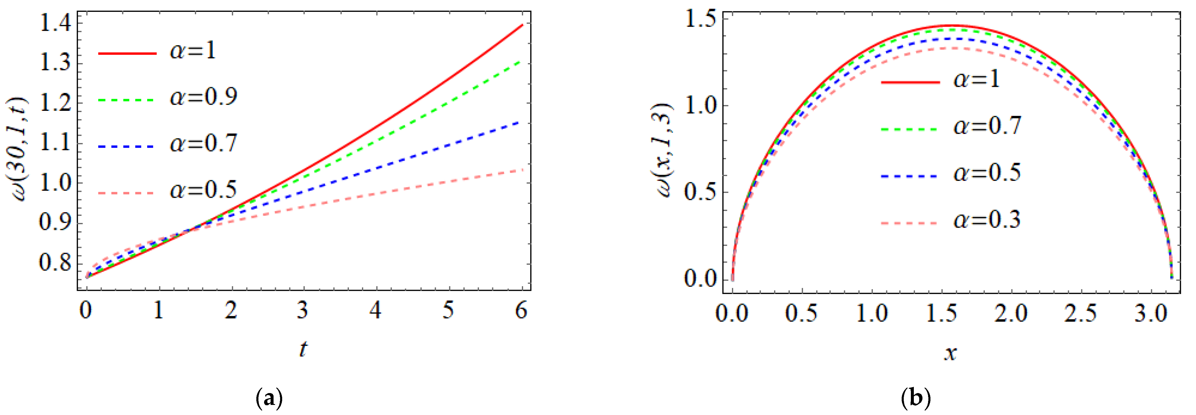
Next, the agreement between the exact and fifth FSS for nonlinear time-FBPM (27) is achieved by calculating the absolute errors ω - ω 5 at ordinary order α = 1 , as in Table 4. Furthermore, Figure 2 exhibits the matching of the geometric behaviour between the exact and FSS solutions at diverse values of the fractional parameter α . Furthermore, Figure 3 shows the impact of fractional derivative on the obtained FSS solutions over α 0,1 , at fixed values of x , and y .
Application 3. 
Consider the nonlinear time-FGBPM given as:
D t α ω = D x 2 ω 2 + D y 2 ω 2 + ω 1 - r ω ,   α 0,1 ,
This model is a special case of nonlinear time-FGBPM (2), where p = q = 1 and λ = 1 . Thus, using the last discussion in Section 3, the LT of (32) could be written as:
W x , y , ξ = ω 0 ( x , y ) ξ + 1 ξ α L L - 1 D x 2 W x , y , ξ 2 + 1 ξ α L L - 1 D y 2 W x , y , ξ 2 + 1 ξ α W x , y , ξ - r ξ α L L - 1 W x , y , ξ 2 .
Utilizing the Laplace FPSM, the j -th Laplace FE series of (33) is given by:
W j x , y , ξ = m = 0 j ω m x , y ξ m α + 1 ξ > 0 ,
and the j -th truncated L-REF of (34) can be identified as:
L R e s W j x , y , ξ = m = 1 j ω m x , y ξ m α + 1 - 1 ξ α L L - 1 D x 2 m = 0 j ω m x , y ξ m α + 1 2 - 1 ξ α L L - 1 D y 2 m = 0 j ω m x , y ξ m α + 1 2 - 1 ξ α m = 0 j ω m x , y ξ m α + 1 + r ξ α L L - 1 m = 0 j ω m x , y ξ m α + 1 2 .
Then, after some algebraic simplifications, we obtain:
L R e s W j x , y , ξ = r ξ - α m = 0 j ξ - m α - 1 Γ ( m α + 1 ) i = m a x ( 0 , m - j ) m i n ( j , m ) ω i ( x , y ) ω n - i ( x , y ) Γ ( i α + 1 ) Γ ( ( m - i ) α + 1 ) - ξ - α ( m = 0 j ξ - m α - 1 Γ ( m α + 1 ) i = max 0 , m - j min j , m 2 D y ω i x , y D y ω j - i - 1 x , y + D y 2 ω i x , y ω - i + j - 1 x , y + ω i x , y D y 2 ω j - i - 1 x , y Γ i α + 1 Γ - i + j - 1 α + 1 ) - ξ - α ( m = 0 j ξ - m α - 1 Γ ( m α + 1 ) i = max 0 , m - j min j , m 2 D x ω i x , y D x ω j - i - 1 x , y + D x 2 ω i x , y ω - i + j - 1 x , y + ω i x , y D x 2 ω j - i - 1 x , y Γ i α + 1 Γ - i + j - 1 α + 1 ) - ξ - α m = 0 j ξ - m α - 1 ω m x , y + m = 1 j ξ - m α - 1 ω m x , y .
Thereafter, we multiply both sides of (36) by the factor ξ j α + 1 , and putting m = j - 1 and m = j with some symbolic simplification, we conclude that:
ξ j α + 1 L R e s W j x , y , ξ = Γ ( ( j - 1 ) α + 1 ) ( r i = 0 j - 1 ω i ( x , y ) ω - i + j - 1 ( x , y ) Γ ( i α + 1 ) Γ ( ( - i + j - 1 ) α + 1 ) - i = 0 j - 1 2 D y ω i x , y D y ω j - i - 1 x , y + D y 2 ω i x , y ω - i + j - 1 x , y + ω i x , y D y 2 ω j - i - 1 x , y Γ i α + 1 Γ - i + j - 1 α + 1 - i = 0 j - 1 2 D x ω i x , y D x ω j - i - 1 x , y + D x 2 ω i x , y ω - i + j - 1 x , y + ω i x , y D x 2 ω j - i - 1 x , y Γ i α + 1 Γ - i + j - 1 α + 1 ) - ω j - 1 ( x , y ) + ω j ( x , y ) .
Solving the resulting equation for ω j ( x , y ) yields the following recurrence relation for j 1 :
ω j x , y = ω j - 1 x , y - Γ j - 1 α + 1 ( r i = 0 j - 1 ω i x , y ω - i + j - 1 x , y Γ i α + 1 Γ - i + j - 1 α + 1 + i = 0 j - 1 2 D y ω i x , y D y ω j - i - 1 x , y + D y 2 ω i x , y ω - i + j - 1 x , y + ω i x , y D y 2 ω j - i - 1 x , y Γ i α + 1 Γ - i + j - 1 α + 1 + i = 0 j - 1 2 D x ω i x , y D x ω j - i - 1 x , y + D x 2 ω i x , y ω - i + j - 1 x , y + ω i x , y D x 2 ω j - i - 1 x , y Γ i α + 1 Γ - i + j - 1 α + 1 ) .
Following the recurrence relation (38) and using the initial data ω x , y , 0 = 1 2 r 2 ( x + y ) , we have the unknown functions ω j x , y = 1 2 r 2 ( x + y ) for j 1 . Thereby, the first few terms of the j -th Laplace FE series for the Laplace Equation (33) are given in the following expansions:
W 1 x , y , ξ = 1 2 r 2 ( x + y ) + 1 2 r 2 ( x + y ) ξ α + 1 ,
W 3 x , y , ξ = 1 2 r 2 ( x + y ) + 1 2 r 2 ( x + y ) ξ α + 1 + 1 2 r 2 ( x + y ) ξ 2 α + 1 + 1 2 r 2 ( x + y ) ξ 3 α + 1 ,
W 4 x , y , ξ = 1 2 r 2 ( x + y ) + 1 2 r 2 ( x + y ) ξ α + 1 + 1 2 r 2 ( x + y ) ξ 2 α + 1 + 1 2 r 2 ( x + y ) ξ 3 α + 1 + 1 2 r 2 ( x + y ) ξ 4 α + 1 ,
W 5 x , y , ξ = 1 2 r 2 ( x + y ) + 1 2 r 2 ( x + y ) ξ α + 1 + 1 2 r 2 ( x + y ) ξ 2 α + 1 + 1 2 r 2 ( x + y ) ξ 3 α + 1 + 1 2 r 2 ( x + y ) ξ 4 α + 1 + 1 2 r 2 ( x + y ) ξ 5 α + 1 .
In the same manner, the rest of the j -th Laplace FSS for each j 6 for the LT Equation (33) can be created. Therefore, the Laplace FE series W x , y , ξ could be created in the following series shape:
W x , y , ξ = lim j W j x , y , ξ = 1 2 r 2 ( x + y ) m = 0 1 ξ m α + 1 ξ > 0 .
Consequently, the analytical approximate FSS of the nonlinear time-FGBPM (32) could be achieved via running the inverse LT on (39) as:
ω x , y , t = 1 2 r 2 ( x + y ) m = 0 t α m Γ m α + 1 = 1 2 r 2 ( x + y ) E α t α .
Correspondingly, the analytical approximate FSS (40) for integer order α = 1 reduces to the exact solution:
ω x , y , t = 1 2 r 2 ( x + y ) m = 0 t m Γ m + 1 = 1 2 r 2 x + y + t ,
which is the same result as the standard problem given in the literature [19].
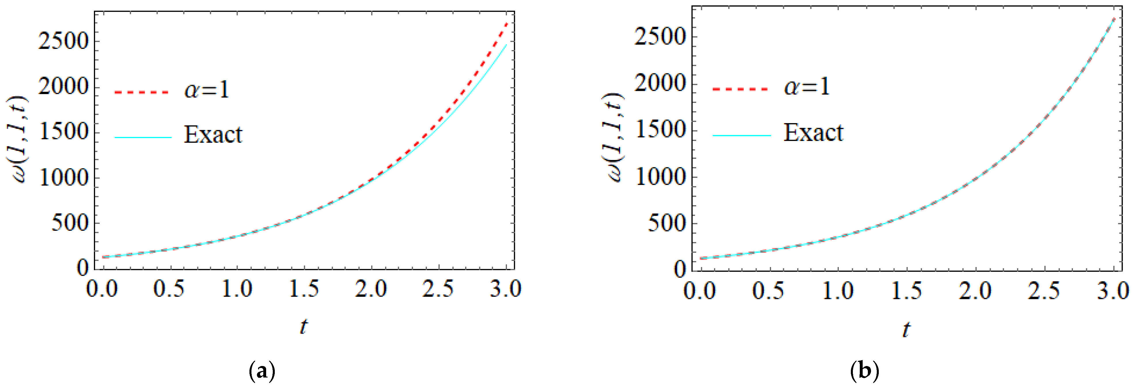
Table 5 exhibits comparisons of ω - ω j of the gained FSS at standard order α . It is evident from the tabulated comparisons that the FSS quickly converges to the exact solution when adding extra FSS terms. Figure 4 shows the geometric behavior of the gained analytical approximate solution at diverse values of parameter α , as well as shows the profile solutions of the analytical approximate solution against the exact solution in standard order. Moreover, the profile of the obtained j th-FSS against the exact solution has been plotted in two dimensions, as in Figure 5. From solution graphics, it is clear that the harmony between the α -th curves analytical approximate solution (40) and the consistency between the exact and the obtained results confirms the accuracy and efficiency of Laplace FPSM. The higher accuracy can be achieved by adding FSS terms.
Application 4. 
Consider the non-linear time-FGBPM given as:
D t α ω = D x 2 ω 2 + D y 2 ω 2 + λ ω - 1 1 - r ω ,   α 0 , 1 ,
In this application, we consider p = - 1 , and q = 1 . Before start applying the Laplace FPSM, assume that f ω = 1 ω ( x , y , t ) - r . So, the non-linear time-FGBPM (42) could be reformulated as:
D t α ω = D x 2 ω 2 + D x 2 ω 2 + λ f = 0 .
Now, we take the LT into (43) such that:
W x , y , ξ = ω 0 ( x , y ) ξ + 1 ξ α L L - 1 D x 2 W x , y , ξ 2 + 1 ξ α L L - 1 D y 2 W x , y , ξ 2 + λ ξ α L { f ω ( x , y , t ) } .
where
W x , y , ξ = m = 0 ω m x , y ξ m α + 1 ξ > 0 .
Following the same fashion as in the last discussion of Application 3, the j -th unknown functions ω j x , y are given the following recurrence formula:
ω j x , y = λ f j - 1 x , y - Γ j - 1 α + 1 ( r i = 0 j - 1 ω i x , y ω - i + j - 1 x , y Γ i α + 1 Γ - i + j - 1 α + 1 + i = 0 j - 1 2 D y ω i x , y D y ω j - i - 1 x , y + D y 2 ω i x , y ω - i + j - 1 x , y + ω i x , y D y 2 ω j - i - 1 x , y Γ i α + 1 Γ - i + j - 1 α + 1 + i = 0 j - 1 2 D x ω i x , y D x ω j - i - 1 x , y + D x 2 ω i x , y ω - i + j - 1 x , y + ω i x , y D x 2 ω j - i - 1 x , y Γ i α + 1 Γ - i + j - 1 α + 1 ) ,
where
ω 0 x , y = 5 + 1 4 λ r x 2 + y + 1 4 λ r y 2 , f j x , y = - 1 ω 0 x , y i = 0 j - 1 f i x , y ω j - i x , y Γ - i + j - 1 α + 1 + r ω j x , y Γ j α + 1 .
Depending on (45) and (46), one can find out the Laplace FE series of (44) as:
W x , y , ξ = ( 5 + 1 4 λ r x 2 + y + 1 4 λ r y 2 + λ 5 + 1 4 λ r x 2 + y + 1 4 λ r y 2 1 ξ 2 α + 1 - λ 2 5 + 1 4 λ r x 2 + y + 1 4 λ r y 2 3 / 2 Γ α + 1 1 ξ 2 α + 1 + ω 3 x , y ξ 3 α + 1 + ω 4 x , y ξ 4 α + 1 + ) ,
Hence, the analytical approximate FSS of the nonlinear time-FGBPM (42) could be achieved via running the inverse LT on (47) as:
ω x , y , t = 5 + 1 4 λ r x 2 + y + 1 4 λ r y 2 + λ t α 5 + 1 4 λ r x 2 + y + 1 4 λ r y 2 Γ α + 1 - λ 2 t 2 α 5 + 1 4 λ r x 2 + y + 1 4 λ r y 2 3 / 2 Γ α + 1 Γ 2 α + 1 + ω 3 x , y Γ 3 α + 1 t 3 α + ω 4 x , y Γ 4 α + 1 t 4 α + .
To highlight comparisons concerning the analytical approximate FSS obtained via our method and test their accuracy, the residual errors are computed for the third truncated FSS for some different values of α , where the residual error of the third analytical approximate FSS of nonlinear time-FGBPM (42) is defined as:
R e s . E r . x , y , t = D t α ω 3 x , y , t - D x 2 ω 3 2 x , y , t - D y 2 ω 3 2 x , y , t - λ ω 3 - 1 x , y , t + λ r .
Table 6 illustrates the numerical comparisons of the residual errors of the third analytical approximate FSS of nonlinear time-FGBPM (42) at various values of fractional order α and some selected points t with fixed values of ( x , y ) . The summarized data provided in this table emphasize the performance of our method and the precision of the obtained third analytical approximate FSS. Geometrically, the behavior of the third analytical approximate FSS at diverse values of fractional parameter α against the exact solution has been illustrated in the two-dimensional graph, as in Figure 6. This figure presents the impact of α on the solution curves, which shows a good agreement between the exact solutions and the obtained results.

5. Conclusions

This work adopted the Laplace FPSM for generating the analytic exact and approximate solutions of nonlinear time-FGBPMs in terms of the time-Caputo fractional derivative. Based on an LT operator and simulation of FPSM, the analytical approximation was constructed for the posed models without imposing any physical restrictive and with few sizes of computational algebraic iterations. The merit of the recommended scheme is to increase the accuracy of FPSM by blending the LT operator in its principal methodology in the construction of the multivariate FSS as a quickly convergent series with the help of the limit concept and ignoring the fractional differentiation. The applicability of our recommended scheme was shown via performing four applications of FGBPM, and the accuracy was checked using numerical error analyses. The profile representations of multivariate FSS and exact solutions were plotted via 2D and 3D surfaces. From numerical and graphical simulations, it was found that FSS behavior is compatible at various fractional derivative values and consistent with the ordinary order. This behavior confirms the effectiveness and accuracy of the presented scheme. Hence, the Laplace FPSM is a speedy, straightforward, and powerful tool that can be modified for novel solutions when approaching biological and dynamical fractional models.

Author Contributions

Conceptualization, M.A. and A.-K.A.; methodology, M.A. and N.T.; software, A.-K.A. and M.A.; validation, A.I. and N.T.; writing—original draft preparation, M.A.; writing—review and editing, A.I., N.T. and A.-K.A.; funding acquisition, A.I. All authors have read and agreed to the published version of the manuscript.

Funding

This work was supported by the Universiti Kebangsaan Malaysia (DIP-2020-001).

Data Availability Statement

Not applicable.

Conflicts of Interest

The authors declare no conflict of interest.

References

  1. Mainardi, F.; Raberto, M.; Gorenflo, R.; Scalas, E. Fractional calculus and continuous-time finance II: The waiting-time distribution. Phys. A Stat. Mech. Its Appl. 2000, 287, 468–481. [Google Scholar] [CrossRef]
  2. Oldham, K.B.; Spanier, J. The Fractional Calculus. Integrations and Differentiations of Arbitrary Order; Academic Press: Cambridge, MA, USA, 1974. [Google Scholar]
  3. Podlubny, I. Fractional Differential Equations; Academic Press: Cambridge, MA, USA, 1999. [Google Scholar]
  4. Atangana, A.; Baleanu, D. New fractional derivatives with nonlocal and non-sin- gular kernel: Theory and application to heat transfer model. Therm. Sci. 2016, 20, 763–769. [Google Scholar] [CrossRef]
  5. Doungmo Goufo, E.F.; Kumar, S.; Mugisha, S.B. Similarities in a fifth-order evolution equation with and with no singular kernel. ChaosSolitons Fractals 2020, 130, 109467. [Google Scholar] [CrossRef]
  6. Ghanbari, B.; Kumar, S.; Kumar, R. A study of behaviour for immune and tumor cells in immunogenetic tumour model with non-singular fractional derivative. ChaosSolitons Fractals 2020, 133, 109619. [Google Scholar] [CrossRef]
  7. Khan, A.M.; Purohit, S.D.; Dave, S.; Suthar, D.L. Fractional mathematical modelling of degradation of dye in textile effluents. Math. Eng. Sci. Aerosp. 2021, 12, 733–741. [Google Scholar]
  8. Alabedalhadi, M.; Al-Smadi, M.; Abu Arqub, O.; Baleanu, D.; Momani, S. Structure of optical soliton solution for nonlinear resonant space-time Schrödinger equation in conformable sense with full nonlinearity term. Phys. Scr. 2020, 95, 105215. [Google Scholar] [CrossRef]
  9. Erturk, V.S.; Alomari, A.K.; Kumar, P.; Murillo-Arcila, M. Analytic solution for the strongly nonlinear multi-order fractional version of a BVP occurring in chemical reactor theory. Discret. Dyn. Nat. Soc. 2022, 2022, 8655340. [Google Scholar] [CrossRef]
  10. Jleli, M.; Kumar, S.; Kumar, R.; Samet, B. Analytical approach for time fractional wave equations in the sense of Yang-Abdel-Aty-Cattani via the homotopy perturbation transform method. Alex. Eng. J. 2020, 59, 2859–2863. [Google Scholar] [CrossRef]
  11. Jaradat, A.; Noorani, M.S.M.; Alquran, M.; Jaradat, H.M. A novel method for solving caputo-time-fractional dispersive long wave wu-zhang system. Nonlinear Dyn. Syst. Theory 2018, 18, 182–190. [Google Scholar]
  12. Al-Smadi, M.; Abu Arqub, O.; Zeidan, D. Fuzzy fractional differential equations under the Mittag-Leffler kernel differential operator of the ABC approach: Theorems and applications. Chaos Solitons Fractals 2021, 146, 110891. [Google Scholar] [CrossRef]
  13. Alaroud, M.; Al-Smadi, M.; Ahmad, R.R.; Salma Din, U.K. Computational optimization of residual power series algorithm for certain classes of fuzzy fractional differential equations. Int. J. Differ. Equ. 2018, 2018, 8686502. [Google Scholar] [CrossRef]
  14. Al-Smadi, M. Fractional residual series for conformable time-fractional Sawada–Kotera–Ito, Lax, and Kaup–Kupershmidt equations of seventh order. Math. Methods Appl. Sci. 2021. Early View. [Google Scholar] [CrossRef]
  15. Abassy, T.A.; El-Tawil, M.A.; El-Zoheiry, H. Toward a modified variational iteration method. J. Comput. Appl. Math. 2007, 207, 137–147. [Google Scholar] [CrossRef]
  16. Wazwaz, A.M. The variational iteration method for solving linear and nonlinear ODEs and scientific models with variable coefficients. Cent. Eur. J. Eng. 2014, 4, 64–71. [Google Scholar] [CrossRef]
  17. Shi, J.; Zhang, N.; Liu, X. A novel fractional wavelet transform and its applications. Sci. China Inf. Sci. 2012, 55, 1270–1279. [Google Scholar] [CrossRef]
  18. Liao, S. Homotopy Analysis Method in Nonlinear Differential Equations; Higher Education Press: Beijing, China, 2012. [Google Scholar]
  19. Arafa, A.A.M.; Rida, S.Z.; Mohamed, H. Homotopy analysis method for solving biological population model. Commun. Theor. Phys. 2011, 56, 797. [Google Scholar] [CrossRef]
  20. Shqair, M.; Alabedalhadi, M.; Al-Omari, S.; Al-Smadi, M. Abundant Exact travelling wave solutions for a fractional massive thirring model using extended Jacobi elliptic function method. Fractal Fract. 2022, 6, 252. [Google Scholar] [CrossRef]
  21. Aljarrah, H.; Alaroud, M.; Ishak, A.; Darus, M. Adaptation of residual-error series algorithm to handle fractional system of partial differential equations. Mathematics 2021, 9, 2868. [Google Scholar] [CrossRef]
  22. Bataineh, M.; Alaroud, M.; Al-Omari, S.; Agarwal, P. Series Representations for Uncertain Fractional IVPs in the Fuzzy Conformable Fractional Sense. Entropy 2021, 23, 1646. [Google Scholar] [CrossRef]
  23. Al-Smadi, M.; Abu Arqub, O.; Hadid, S. Approximate solutions of nonlinear fractional Kundu-Eckhaus and coupled fractional massive Thirring equations emerging in quantum field theory using conformable residual power series method. Phys. Scr. 2020, 95, 105205. [Google Scholar] [CrossRef]
  24. Lu, Y.G. Hölder estimates of solutions of biological population equations. Appl. Math. Lett. 2000, 13, 123–126. [Google Scholar] [CrossRef]
  25. Gurtin, M.E.; MacCamy, R.C. On the diffusion of biological populations. Math. Biosci. 1977, 33, 35–49. [Google Scholar] [CrossRef]
  26. Bear, J. Dynamics of Fluids in Porous Media; American Elsevier: New York, NY, USA, 1972. [Google Scholar]
  27. Shakeri, F.; Dehghan, M. Numerical solution of a biological population model using He’s variational iteration method. Comput. Math. Appl. 2007, 54, 1197–1209. [Google Scholar] [CrossRef]
  28. Singh, B.K. A novel approach for numeric study of 2D biological population model. Cogent Math. 2016, 3, 1261527. [Google Scholar] [CrossRef]
  29. Srivastava, V.K.; Kumar, S.; Awasthi, M.K.; Singh, B.K. Two-dimensional time fractional-order biological population model and its analytical solution. Egypt. J. Basic Appl. Sci. 2014, 1, 71–76. [Google Scholar] [CrossRef]
  30. Roul, P. Application of homotopy perturbation method to biological population model. Appl. Appl. Math. Int. J. 2010, 5, 272–281. [Google Scholar]
  31. El-Ajou, A. Adapting the Laplace transform to create solitary solutions for the nonlinear time-fractional dispersive PDEs via a new approach. Eur. Phys. J. Plus. 2021, 136, 229. [Google Scholar] [CrossRef]
  32. Amryeen, R.; Harun, F.N.; Al-Smadi, M.; Alias, A. Adaptation of conformable residual series algorithm for solving temporal fractional gas dynamics models. Arab J. Basic Appl. Sci. 2022, 29, 65–76. [Google Scholar]
  33. Aljarrah, H.; Alaroud, M.; Ishak, A.; Darus, M. A Novel Analytical LRPSM for Solving Nonlinear Systems of FPDEs. Fractal Fract. 2022, 6, 650. [Google Scholar] [CrossRef]
  34. Aljarrah, H.; Alaroud, M.; Ishak, A.; Darus, M. Approximate solution of nonlinear time-fractional PDEs by Laplace residual power series method. Mathematics 2022, 10, 1980. [Google Scholar] [CrossRef]
  35. Burqan, A.; El-Ajou, A.; Saadeh, R.; Al-Smadi, M. A new efficient technique using Laplace transforms and smooth expansions to construct a series solution to the time-fractional Navier-Stokes equations. Alex. Eng. J. 2022, 61, 1069–1077. [Google Scholar] [CrossRef]
  36. Al-Zhour, Z.; El-Ajou, A.; Oqielat, M.A.N.; Al-Oqily, O.N.; Salem, S.; Imran, M. Effective approach to construct series solutions for uncertain fractional differential equations. Fuzzy Inf. Eng. 2022. Published online. [Google Scholar] [CrossRef]
  37. Prakasha, D.G.; Veeresha, P.; Baskonus, H.M. Residual power series method for fractional Swift–Hohenberg equation. Fractal Fract. 2019, 3, 9. [Google Scholar] [CrossRef]
  38. Alaroud, M.; Al-Smadi, M.; Rozita Ahmad, R.; Salma Din, U.K. An analytical numerical method for solving fuzzy fractional Volterra integro-differential equations. Symmetry 2019, 11, 205. [Google Scholar] [CrossRef] [Green Version]
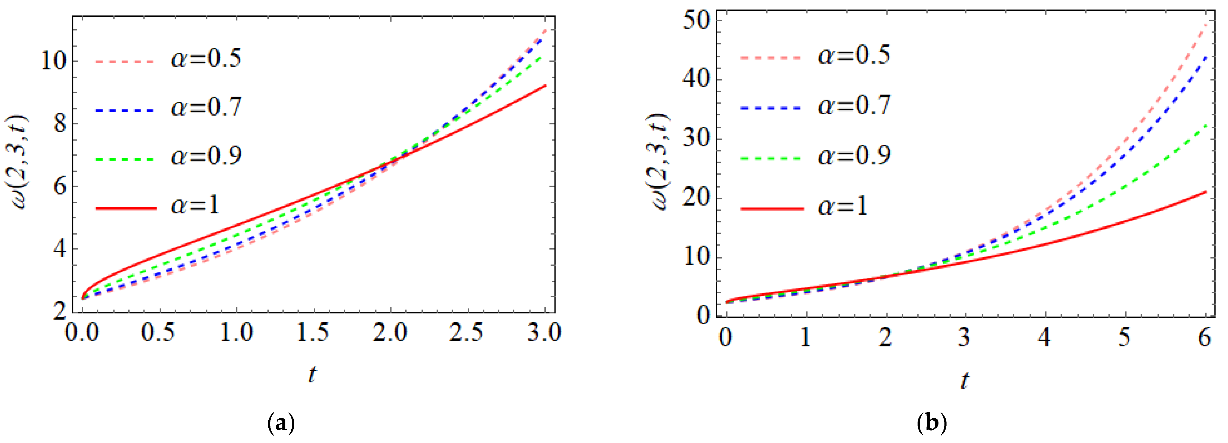
Figure 1. The behaviour of the analytical approximate FSS for nonlinear time-FBPM (15) at various values of α and λ = 0.5 ; (a) for t [ 0 , 3 ] , (b) for t [ 0 , 6 ] .
Fractalfract 07 00176 g001
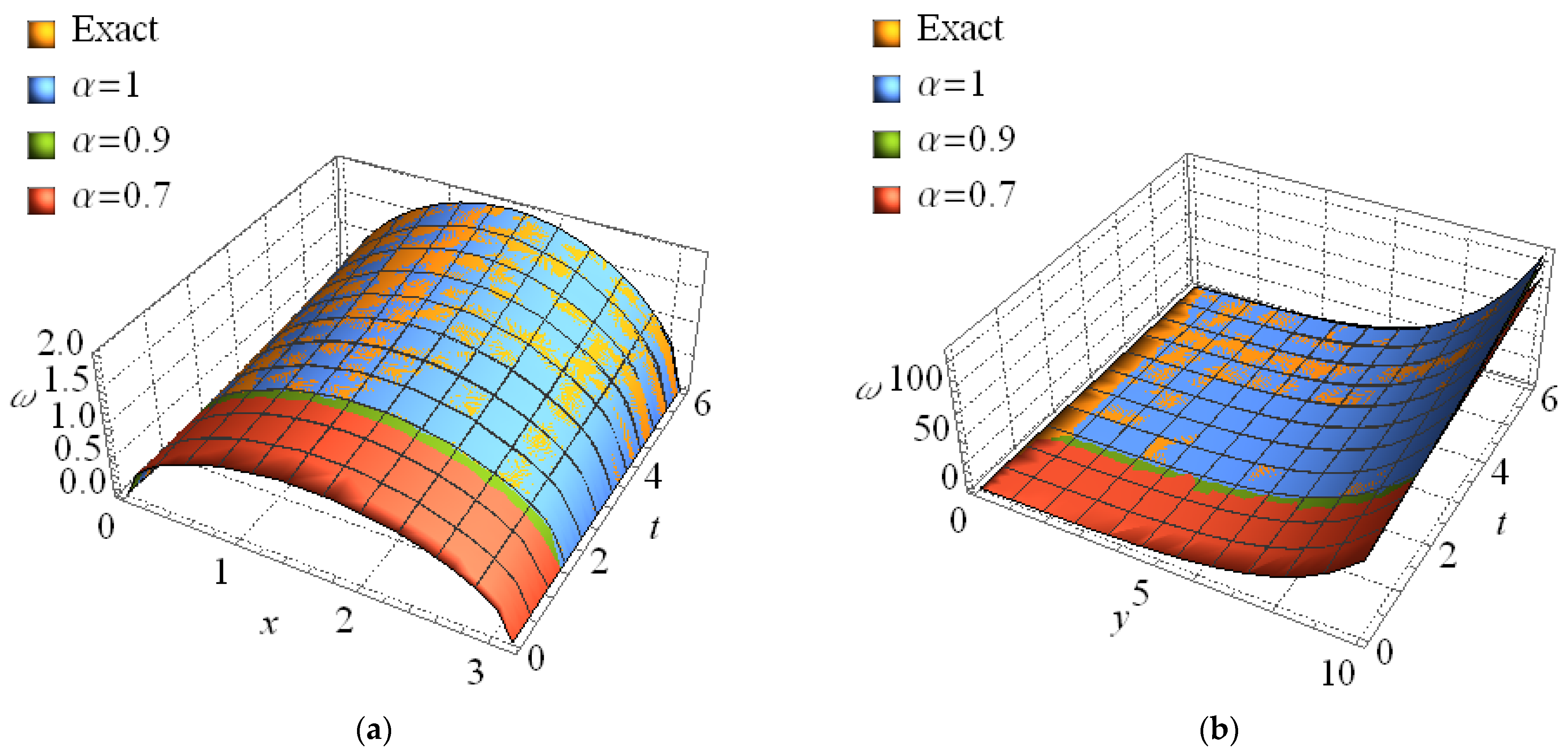
Figure 2. The 3D plots of the α -th curve FSS for the nonlinear time-FBPM (28) for α 1 , 0.9 , 0.7 , 0.5 and λ = 0.1 ; (a) for y = 1 , (b) for x = π 2 .
Fractalfract 07 00176 g002
Figure 3. The geometric behaviour of α -th curve FSS for the nonlinear time-FBPM (28) at different values α ( 0 , 1 ] and λ = 0.1 ; (a) for x = 30 , y = 1 , (b) for y = 1 , t = 1 .
Fractalfract 07 00176 g003
Figure 4. (a) Behavior of α -th curve analytical approximate solution (40) for all t 0 , 3 and α 1 , 0.9 , 0.7 , 0.5 , (b) behavior of exact solution versus the analytical approximate solution (40) for all t 0 , 3 .
Fractalfract 07 00176 g004
Figure 5. The behavior of exact versus j -th analytical approximate solutions for all t 0 , 3 , (a) For j = 5 ; (b) For j = 10 .
Fractalfract 07 00176 g005
Figure 6. Profile exact and 3rd FSS solutions for nonlinear time-FGBPM (42) at various values of α for all t 0 , 6 . (a) For x = y = 10 , (b) For x = y = 2 .
Fractalfract 07 00176 g006
Table 1. Comparison of absolute errors of the nonlinear time-FBPM (15).
t ω - ω 6 ω - ω 12 ω - ω 18
0.5 3.061708664375828 × 10 - 8 4.44089209850063 × 10 - 16 4.440892098500626 × 10 - 16
1 4.048135929579644 × 10 - 6 4.97379915032070 × 10 - 14 0.0
1.5 7.150407740663667 × 10 - 5 9.87299131338659 × 10 - 12 8.881784197001252 × 10 - 16
2 5.542531561681940 × 10 - 4 4.23460377874108 × 10 - 10 0.0
2.5 2.736956864421103 × 10 - 3 7.851848948803308 × 10 - 9 1.776356839400250 × 10 - 15
3 1.016540163180935 × 10 - 2 8.566345144345178 × 10 - 8 4.973799150320701 × 10 - 14
Table 2. Numerical solutions of the 6th FSS for the nonlinear time-FBPM (15).
t i Exact6th-FSS
α = 1 α = 0.95 α = 0.85
0.5 3.145207087649518 3.145207057032432 3.195437680739461 3.306493306455880
1 4.038525841288411 4.038521793152482 4.105554824617641 4.245814688736310
1.5 5.185569826164564 5.185498322087158 5.253448925361035 5.386794675631956
2 6.658403456804333 6.657849203648165 6.708096482666050 6.792504963679339
2.5 8.549559273098282 8.546822316233861 8.553458937008319 8.531511130094565
3 10.97785140813657 10.96768600650476 10.89318588408218 10.68360229862708
Table 3. Numerical solutions of the 12th FSS for the nonlinear time-FBPM (15).
t α = 0.7 α = 0.5 α = 0.3 α = 0.1
0.5 1.4304426170 1.5670592359 1.7436227777 1.9399857896
1 1.8249850566 1.9523604092 2.0620071729 2.0768077222
1.5 2.2750673796 2.3476620568 2.3420796264 2.1709283161
2 2.8038430557 2.7742779826 2.6090467681 2.2453761878
2.5 3.4320723970 3.2440756075 2.8723526367 2.3081488661
3 4.1824947771 3.7667181702 3.1368482479 2.3630675139
Table 4. Numerical results for the non-linear time-FBPM (27) when α = 1 .
x , y , t i ω ω 5 ω - ω 5
30,1 , 1 0.8471699886414954 0.8471699875614395 1.080055933577739 × 10 - 9
30,1 , 2 0.9362676341130575 0.9362675639786114 7.013444602854690 × 10 - 8
30,1 , 3 1.0347357607572423 1.0347349500711882 8.106860540646466 × 10 - 7
30,1 , 4 1.1435598706817850 1.1435552476315374 4.623050247731797 × 10 - 6
30,1 , 5 1.2638291121558574 1.2638112100956973 1.790206016005769 × 10 - 5
30,1 , 6 1.3967471801720195 1.3966929080544292 5.427211759023720 × 10 - 5
Table 5. Comparison of absolute errors of the nonlinear time-FGBPM (32).
t i ω - ω 5 ω - ω 10 ω - ω 15
0.32 1.154399098801662 × 10 - 5 6.82121026329696 × 10 - 13 3.552713678800501 × 10 - 15
0.64 7.752680289705438 × 10 - 4 1.44248701872129 × 10 - 9 1.776356839400250 × 10 - 15
0.96 9.282582583590937 × 10 - 3 1.28346115957356 × 10 - 7 1.918465386552270 × 10 - 13
1.28 5.492411206336811 × 10 - 2 3.12802043822557 × 10 - 6 1.982414232770679 × 10 - 11
1.6 2.210639902097142 × 10 - 1 3.75098779556993 × 10 - 5 7.187210826486990 × 10 - 10
1.92 6.978720380377368 × 10 - 1 2.87291486316121 × 10 - 4 1.3566136658482720 × 10 - 8
Table 6. Comparison of residual errors of the third analytical approximate FSS of nonlinear time-FGBPM (42) at various values of fractional order α .
t i x = y = 2
α = 1 α = 0.75 α = 0.5
0.2 5.283510764314547 × 10 - 10 2.637395913216919 × 10 - 7 6.492114991403855 × 10 - 7
0.4 2.080334098562841 × 10 - 9 4.648777811163893 × 10 - 7 1.016953392316000 × 10 - 6
0.6 4.606681074798002 × 10 - 9 6.6704860020219 × 10 - 7 1.366676980466517 × 10 - 6
0.8 8.058574000810449 × 10 - 9 8.816743810253007 × 10 - 7 1.718134829568028 × 10 - 6
1 1.23876446227536 × 10 - 8 1.114486273705306 × 10 - 6 2.077608461280126 × 10 - 6
t i x = y = 10
α = 1 α = 0.75 α = 0.5
0.2 3.043010288195091 × 10 - 12 1.173598279669008 × 10 - 8 2.623857382755279 × 10 - 8
0.4 1.171023000789972 × 10 - 11 1.963562601403623 × 10 - 8 3.659683277257297 × 10 - 8
0.6 2.531018450380173 × 10 - 11 2.643230756493864 × 10 - 8 4.419687404944028 × 10 - 8
0.8 4.315116319819623 × 10 - 11 3.252796791641810 × 10 - 8 5.031243172082256 × 10 - 8
1 6.454230205843459 × 10 - 11 3.809079993088993 × 10 - 8 5.544396378120986 × 10 - 8
Disclaimer/Publisher’s Note: The statements, opinions and data contained in all publications are solely those of the individual author(s) and contributor(s) and not of MDPI and/or the editor(s). MDPI and/or the editor(s) disclaim responsibility for any injury to people or property resulting from any ideas, methods, instructions or products referred to in the content.